Phase synchronization on scale-free and random networks in the presence of noise

Abstract

In this work we investigate the stability of synchronized states for the Kuramoto model on scale-free and random networks in the presence of white noise forcing. We show that for a fixed coupling constant, the robustness of the globally synchronized state against the noise is dependent on the noise intensity on both kinds of networks. At low noise intensities the random networks are more robust against losing the coherency but upon increasing the noise, at a specific noise strength the synchronization among the population vanishes suddenly. In contrast, on scale-free networks the global synchronization disappears continuously at a much larger critical noise intensity respect to the random networks.

I Introduction

Collective behavior in a population of individuals is of great importance in many areas of physics, biology, social sciences and many other disciplinessync ; bio ; winfree . One of the most celebrated collective behaviors is the case of phase synchronization among a population of interacting self-sustained oscillators, in which all members tend to oscillate coherently with more or less the same phase. A population of coupled phase oscillators with mutual sine interaction between the pairs, is known as the Kuramoto model kuramoto . This model is introduced by Kuramoto  kuramoto1 and has extensively been investigated by many authors (see acebron ; boccaletti ; book1 and references therein).

Considering a network of coupled rotors (phase oscillators), many factors such as coupling strengthcs , time delayed interactions td , individual frequency distributionacebron ; bimodal , topology of network topology and noisesacebron ; noise , affect the path toward the full synchronization.

The synchronization of the deterministic Kuramoto model with random distribution of rotor frequencies and initial phases, has been studied on the scale-free networks by Moreno and Pacheco SFsync . There, it has been shown that the onset of synchronization occurs through a continuous transition at a small value of coupling with a critical exponent near $0.5$. This resembles the mean-field behaviour, except that in the case of scale-free networks the critical coupling at which the rotors begin to get synchronized, is much smaller respect to all-to-all networks. They have also managed to find that in the complete synchronized state, dependence of the recovery time respect to the node degree is a power law function with exponent close to -1, which shows the robustness of highly connected nodes (hubs) against perturbations.

The comparison between the synchronizability of the Kuramoto model on Erdös-Rènyi(ER) and scale-free networks has been carried out recently by Goméz-Gardeñ et al gomez1 ; gomez2 . In these references, the authors have found that while the onset of global synchronization occurs at smaller value of coupling for the scale-free networks, but tendency toward the global coherence grows suddenly to larger extends for ER networks, at higher couplings. The reason for such behaviour is that the giant cluster in the heterogeneous networks (such as scale-free networks), originating from a central core of high connectivity (hub), grows continuously by attaching the smaller clusters to it upon increasing the coupling constant. In contrast, for the homogeneous networks, the evolution toward full synchronization would be boosted up by merging many small clusters spreading uniformly though out the networks, when the coupling is large enough.

In this paper our focus is on the effect of white noise forcing on the synchronization of Kuramoto model for two types of networks: scale-free networks introduced by Barabási and Albert(BA) BA and random networksER . The paper is organized as follows: in section II, we introduce the stochastic Kuramoto model and express briefly some results for all-to-all networks, section III, is devoted to the simulation results and the conclusion will be presented in section IV.

II Stochastic Kuramoto model on a complex network

Consider a system composed of $N$ rotors with the intrinsic frequencies, denoted by $\omega_{i}$, on the top of a complex network consisting of $N$ nodes. The stochastic Kuramoto model on such a network is described by the following set of equations:

$$\frac{d\theta_{i}}{dt}=\omega_{i}+\lambda\sum_{j}a_{ij}\sin(\theta_{j}-\theta_{i})+\eta_{i}(t)\;,\hskip 14.22636pti=1\cdot\cdot\cdot N,$$ (1)

where $\theta_{i}$ is the phase of the rotor on the node $i$, $\lambda$ is the coupling constant and $a_{ij}$ is an element of the connectivity matrix, which takes the value $a_{ij}=1$ if $i$ and $j$ are linked together and $0$ otherwise. $\eta_{i}$ is the random force applying on the $i$-th rotor, and usually is chosen as a white noise with zero mean-value. The spatial-temporal correlation of such a noise is given by:

$$\langle\eta_{i}(t)\eta_{j}(t^{\prime})\rangle=2D\delta(t-t^{\prime})\delta_{ij},$$ (2)

where $D$ is variance of the noise.

The stochastic Kuramoto model on an all-to-all network has been investigated analytically by Acebrón et al acebron , who have shown that taking a one peaked symmetrical frequency distribution $f(\omega)=f(-\omega)$ for oscillators, there would be a critical coupling constant $\lambda_{c}=2/[\pi f(0)]$ above which the network begins to get synchronized. Near this critical point, the order parameter obeys a power law relation, namely

$$r\sim\sqrt{\frac{-16(\lambda-\lambda_{c})}{\pi\lambda_{c}^{4}f^{\prime\prime}(0)}}.$$ (3)

They have also shown that for a Lorentzian frequency distribution $f(\omega)=(\gamma/\pi)/(\omega^{2}+\gamma^{2})$, the incoherent solution is linearly stable for points $(\lambda,D)$ above the critical line $D=-\gamma+\lambda/2$. In terms of coupling strength, this is also linearly stable for $\lambda<\lambda_{c}=2D+2\gamma$.

In the next section we numerically integrate Eq.(1) on scale-free and random networks and compare the results.

III simulation results for scale-free and random networks

To create a scale-free network with average connectivity $\langle k\rangle=2m$, we use the BA algorithm BA . In this procedure, starting from $m_{0}$ initial nodes all connected to each other, at each step one attaches a newly entering node to $m\leq m_{0}$ elder ones such that the nodes with higher connectivity have larger probability (proportional to their degree) to get connected with this new one. Repeating this stages provides us with a network whose degree distribution obeys a power law function as $P(k)\sim k^{-\gamma}$ with $\gamma=3$. For producing ER network composed of $N$ nodes and with the same average degree per node($\langle k\rangle=2m$), it is enough to distribute $Nm$ edges between randomly chosen pair of nodesER .

In this work, we set $m=10$ and select a delta function distribution for intrinsic frequencies, $f(\omega)=\delta(\omega-\omega_{0})$. Changing the reference frame to a rotating one with rotation frequency $\omega_{0}$, enable us to set $\omega_{i}=0$ for all rotors in Eq.(1). We also pick $\eta_{i}(t)$ out of a box distribution in the interval $-g/2<\eta<g/2$, hence its variance is given by $D=\frac{g^{2}}{24}$. Using Ito’s formalism for integration of a stochastic functionito , one obtains the following discrete equation from Eq.(1):

$$\theta_{i}(t+dt)=\theta_{i}(t)+\lambda\left[\sum_{j}a_{ij}\sin(\theta_{j}(t)-\theta_{i}(t))\right]dt+\eta_{i}(t)\sqrt{dt}+O(dt^{2}),$$ (4)

where in the Ito’s picture, $\eta_{i}(t)$ is evaluated at the initial point of the time interval $[t,t+dt]$. Time step, $dt$, is taken small enough to reduce the computational error. The initial values of $\theta_{i}$ are randomly drawn from a uniform distribution in the interval $[-\pi,\pi]$. To characterize the global phase coherency, we define the following order parameter:

$$r(t)=\langle|\frac{1}{N}\sum_{j=1}^{N}e^{i\theta_{i}(t)}|\rangle,$$ (5)

which $\langle\cdot\cdot\cdot\rangle$ means the averaging over different realizations of noise and initial conditions. In the stationary regime the time argument of $r(t)$ can be omitted and one can replace the averaging over realizations by time averaging. The order parameter takes the value $0\leq r\leq 1$, where $r=0$ corresponds to the disordered phase and $r=1$ characterizes the full synchronized state.

In the absence of noise for scale-free network, we found that the rotors get synchronized for a very small value of coupling around $\lambda=0.03$. We choose a large enough value for the coupling to make sure that the system is in the full synchronized state when the noise is turned off, then increase the noise intensity until the global coherency vanishes at the critical value of the noise strength, $g_{c}$.

In addition to the order parameter $r$, for better specifying the transition from coherency to decoherency, we introduce the Binder’s forth cumulant which is defined as:

$$u=1-\frac{\langle r^{4}\rangle}{3\langle r^{2}\rangle^{2}}.$$ (6)

It is easy to see that in coherent phase, where $\langle r\rangle$ is nonzero, $u$ takes the value $2/3$ in the large $N$ limit, while upon vanishing the global synchronization($\langle r\rangle$=0) this quantity falls down to $1/3$ in thermodynamic limit. The much smaller numerical errors in computation of the Binder’s forth cumulant rather than the order parameter, makes it more advantageous for determination of the position and treatment of the coherency-decoherency phase transition.

Figs.1 and 2 represent the time dependence of order parameter for scale-free and random networks composed of $N=10^{4}$ rotors, respectively. To derive these data, we put $dt=0.01$, $\lambda=0.2$ and averagings have carried out over 100 different realizations of noise and initial phase configurations, for the noise intensities increasing from $g=2.0$ by step $\Delta g=2.0$. From these figures, one finds that after about 500 time steps the system reaches the stationary for all noise intensities, and obviously the global coherency vanishes at larger coupling values for the scale-free network (around $g=10.0$) respect to the random network (around $g=8.0$).

In what follows, to find the dependence of the order parameter as well as Binder’s forth cumulant on the noise intensity, we fix the number of nodes to $N=10^{4}$, and the averagings are carried on $10^{4}$ time steps after skipping $2000$ initial steps, where the system is surely in the stationary state.

In Figs.3 and 4 we have depicted the order parameter, $r$, versus the noise intensity, $g$, for scale-free and random networks, for three coupling constants $\lambda=0.1,0.15,0.2$. Similar graphs for the Binder’s forth cumulant, $u$, is represented in Figs.5 and 6.

For comparison, the noise intensity variations of $r$ and $u$ have been depicted for both scale-free and random networks in Figs.7a and 7b.

By inspecting these figures one can extract two essential results:
(i) Synchronizability of each kind of networks depends on the coupling strength, such that at small noise intensities the order parameter for random network falls more slowly than scale-free’s, so it is more robust than SF network against the noise while at large noise intensities the situation is vice versa (see Fig.7a). The critical noise intensity ($g_{c}$) at which the transition from synchronized to un-synchronized state occurs is larger for the scale-free network. So the coherent state in SF network persists more against the noise than the random network with the same average degree and coupling constant.
(ii) The coherency among the population of rotors destroys smoothly by increasing the noise intensity in the scale-free networks, while in the random networks the synchronization disappears by a sudden fall at the transition point. These behaviours are more apparent from the treatment of Binder’s forth cumulant shown in Figs.5, 6 and 7b. Then the order-disorder transition in SF networks resembles the continuous transitions in equilibrium critical phenomena, while the transition in random networks is discontinuous-like.

Referring to Goméz-Gardeñes et algomez1 ; gomez2 , a nice explanation of our results are as follows. In homogeneous systems such as random networks, starting from the fully synchronized phase, when we turn on the noise, some incoherent clusters with more or less the same size begin to form. At low noise intensities, the size of these clusters are small and they are well separated, but by increasing the noise they get larger and connected to each other at intermediate noise intensities. At this point, the locally synchronized regions are not coherent anymore, so a big drop occurs for the order parameter. This is much like the first order phase transitions in equilibrium statistical mechanics, where the ordered and disordered phases coexist at the transition point. On the other hand, the fully coherent state in the SF networks is founded around a core consists of nodes with high connectivity (hubs). When noise is applied on such state, the un-synchronized parts leave this giant cluster one by one, leading to continuous destruction of global coherency.

IV conclusion

In summary, we numerically investigated the stability of the global phase synchronized state in Kuramoto model on the top of scale-free and random networks, under white noise forcing on each oscillator. Our results emphasize on the fact that the stability of the synchronized phase is dependent on the noise strength, such that at low noise intensities the random networks are more stable against loosing the coherency, while at intermediate noise intensities, the coherency falls abruptly in such networks. However, in scale-free networks the coherency among the rotors decreases smoothly and also persists up to larger extends of noise intensity. Therefore, our findings confirm the picture presented by Goméz-Gardeñes et algomez1 ; gomez2 , that in heterogeneous networks the giant cluster formed around a core of hubs, grows (falls) continuously by increasing (decreasing) the coupling or by lowering (rising) the noise intensity. On the contrary, in homogeneous systems such as random networks, by increasing the noise intensity, the coalescence of un-synchronized clusters which are uniformly distributed over the network, results in a sudden fall in the global synchronization at the transition point. So the more complex is a system, more predictable it is.

This work sheds more light on the different aspects of nonlinear dynamics on the top of homogeneous and heterogeneous network topologies and we hope that it promotes more researches on this very interesting problem.

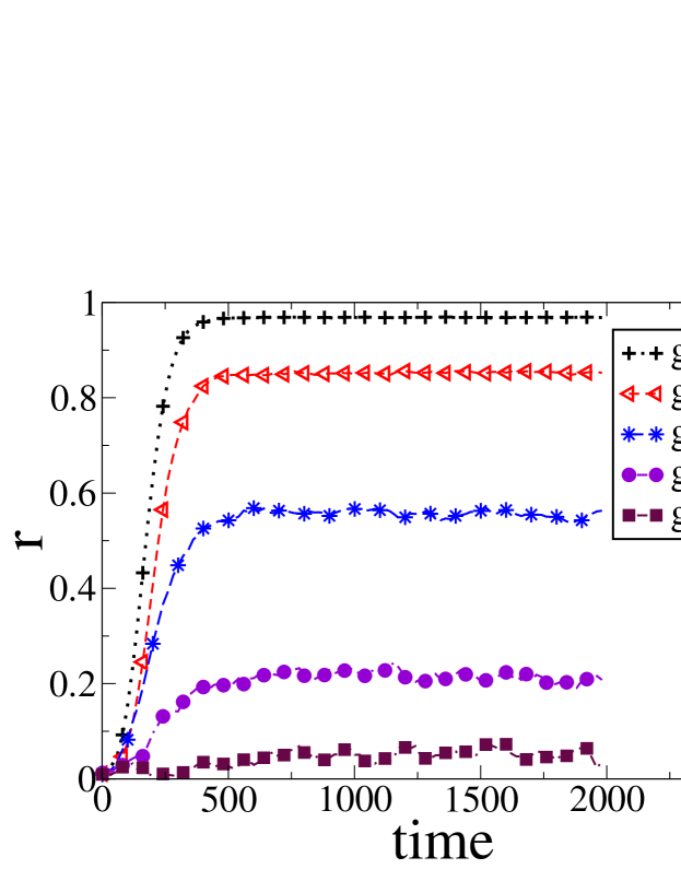
Figure 1: Order parameter versus time for different noise intensities on the scale-free network. The results are obtained for coupling constant $\lambda=0.2$ and the number of nodes is $N=10^{4}$.

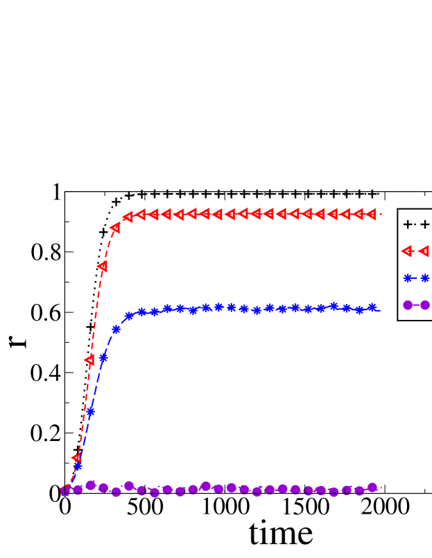
Figure 2: Order parameter versus time for different noise intensities on the random network. The results are obtained for coupling constant $\lambda=0.2$ and the number of nodes is $N=10^{4}$.

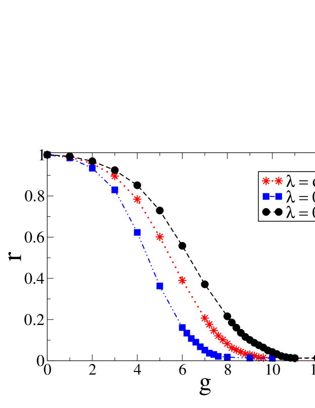
Figure 3: The order parameter versus the noise intensity for the scale-free network. The results are obtained for three coupling values $\lambda=0.1,0.15,0.2$ and $N=10^{4}$ phase oscillators.

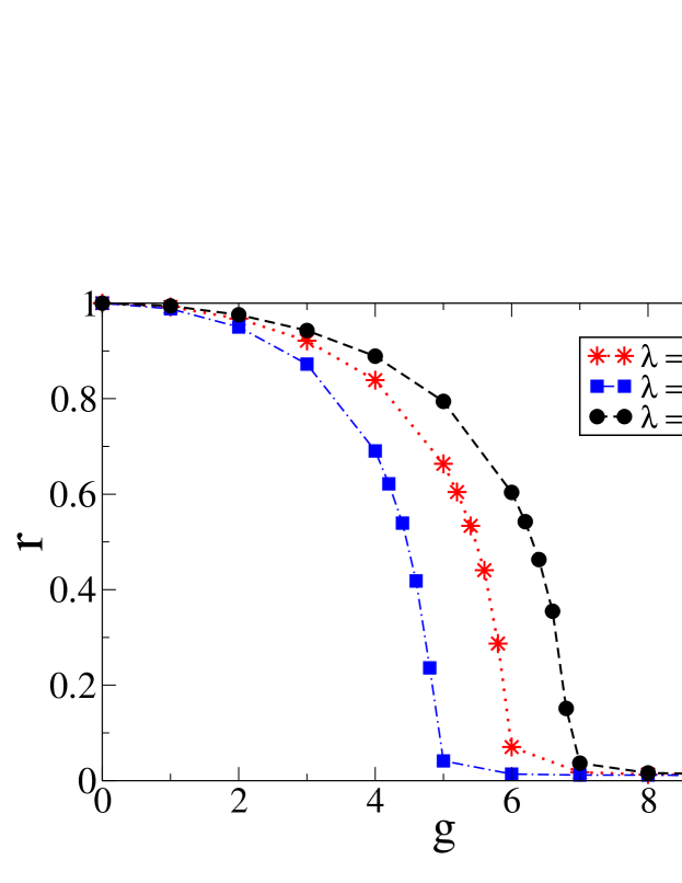
Figure 4: The order parameter versus the noise intensity for the random network. The results are obtained for three coupling values $\lambda=0.1,0.15,0.2$ and $N=10^{4}$ phase oscillators.

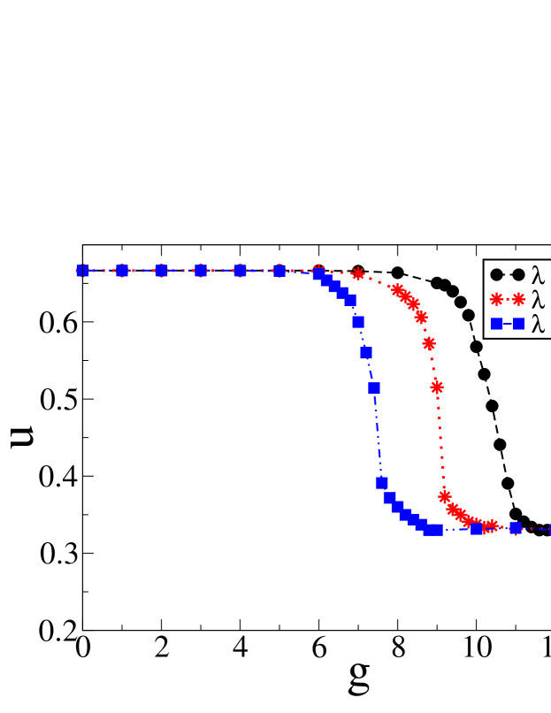
Figure 5: The Binder’s forth cumulant (Eq.6) versus the noise intensity for the scale-free network. The results are obtained for three coupling values $\lambda=0.1,0.15,0.2$ and $N=10^{4}$ phase oscillators.

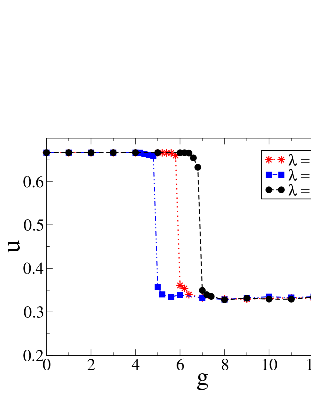
Figure 6: The Binder’s forth cumulant (Eq.6) versus the noise intensity for the random network. The results are obtained for three coupling values $\lambda=0.1,0.15,0.2$ and $N=10^{4}$ phase oscillators.

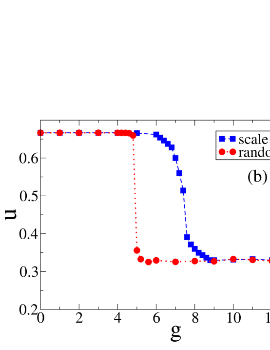
Figure 7: Noise intensity dependence of (a) Order parameter and (b) Binder’s forth cumulant for the scale free and random network at $\lambda=0.1$.

References

- (1) S. H. strogatz, Sync: The emergence science of spontanous order (Hyprion, New York 2003).
- (2) J. D. Murray, Mathematical Biology (Springer, New York, Berlin, Heidelberg 1993).
- (3) A. T. Winfree, The Geometry of Biological Time(Springer, New York, 1980 )
- (4) Y. Kuramoto, Physica D 50, 15 (1991).
- (5) Y. Kuramoto, in International Symposium on Mathematical Problems in heoretical Physics, edited by H. Araki, Lecture Notes in Physics No. 30 (Springer, New York, 1975), p. 420.
- (6) J. A. Acebrón, L. L. Bonilla, and R. spigler, Rev. Mod. Phys. 77, 137 (2005).
- (7) J. A. Acebrón, L. L. Bonilla, S. De Leo, and R. Spigler, Phys. Rev. E 57, 5287 (1998).
- (8) S. Boccaletti, V. Latora, Y. Moreno, M. Chavez and D. U.-U.Hwang, Physics Reports, 424, 175 (2006).
- (9) A. Pikovsky, M. Rosenblum, and J. Kurths, Synchronization, A universal concept in nonlinear sciences (Cambridge University Press, UK, 2003).
- (10) M. Chavez, D.-U. Hwang, A. Amann, H.G. Henstchel, and S. Boccaletti 94, 218701 (2005).
- (11) T. B. Luyzanina, Networks: Computation in Neural systems 6, 43 (1995); M. G. Earl and S. H. Strogatz, Phys. Rev. E 67, 036204(2003); H. G. Schuster and P. Wagner, Prog. Theor. Phys 81, 929 (1989); E. Niebur, H. G. Schuster and D. M. Kammen, Phys. Rev. Lett. 67, 2753 (1991).
- (12) L. Donetti, P. I. Hurtado, and M. A. Muñoz, Phys. Rev. Lett. 95, 188701 (2005); M. Timme, F. Wolf, and T. Geisel, Phys. Rev. Lett. 92, 074101 (2004); A. Arenas, A. Díaz-Guilera, and C. J. Pérez-Vicente, Phys. Rev. Lett. 96, 114102 (2006).
- (13) L. L. Bonilla, J. C. Neu, and R. Spigler, Journal of Statistical Physics 67, 313 (1992).
- (14) A. L. Barabási, and R. Albert, Science 286, 509 (1999); A. L. Barabasi, R. Albert, and H. Joeng, Physica A 272, 173 (1999).
- (15) P. Erdös and A. Rényi, Publ. Math. Debrecen 6, 290 (1959); Publ. Math. Inst. Hung. Acad. Sci 5, 17 (1960).
- (16) Y. Moreno and A. F. Pacheco, Europhysics Letters 68, 603 (2004).
- (17) J. Goméz-Gardeñes, Y. Moreno, and A. Arenas, Phys. Rev. Lett. 98, 034101 (2007).
- (18) J. Goméz-Gardeñes, Y. Moreno, and A. Arenas, Phys. Rev. E 75, 066106 (2007).
- (19) C. W. Gardiner, Handbook of Stochastic Methods for Physics, Chemistry and the Natural Sciences, (Springer-Verlag, 1980).