Bayesian Inference on Mixtures of Distributions

Abstract

This survey covers state-of-the-art Bayesian techniques for the estimation of mixtures. It complements the earlier Marin et al., (2005) by studying new types of distributions, the multinomial, latent class and $t$ distributions. It also exhibits closed form solutions for Bayesian inference in some discrete setups. Lastly, it sheds a new light on the computation of Bayes factors via the approximation of Chib, (1995).

1 Introduction

Mixture models are fascinating objects in that, while based on elementary distributions, they offer a much wider range of modeling possibilities than their components. They also face both highly complex computational challenges and delicate inferential derivations. Many statistical advances have stemmed from their study, the most spectacular example being the EM algorithm. In this short review, we choose to focus solely on the Bayesian approach to those models (Robert and Casella, 2004). Frühwirth-Schnatter, (2006) provides a book-long and in-depth coverage of the Bayesian processing of mixtures, to which we refer the reader whose interest is woken by this short review, while MacLachlan and Peel, (2000) give a broader perspective.

Without opening a new debate about the relevance of the Bayesian approach in general, we note that the Bayesian paradigm (see, e.g., Robert, 2001) allows for probability statements to be made directly about the unknown parameters of a mixture model, and for prior or expert opinion to be included in the analysis. In addition, the latent structure that facilitates the description of a mixture model can be naturally aggregated with the unknown parameters (even though latent variables are not parameters) and a global posterior distribution can be used to draw inference about both aspects at once.

This survey thus aims to introduce the reader to the construction, prior modelling, estimation and evaluation of mixture distributions within a Bayesian paradigm. Focus is on both Bayesian inference and computational techniques, with light shed on the implementation of the most common samplers. We also show that exact inference (with no Monte Carlo approximation) is achievable in some particular settings and this leads to an interesting benchmark for testing computational methods.

In Section 2, we introduce mixture models, including the missing data structure that originally appeared as an essential component of a Bayesian analysis, along with the precise derivation of the exact posterior distribution in the case of a mixture of Multinomial distributions. Section 3 points out the fundamental difficulty in conducting Bayesian inference with such objects, along with a discussion about prior modelling. Section 4 describes the appropriate MCMC algorithms that can be used for the approximation to the posterior distribution on mixture parameters, followed by an extension of this analysis in Section 5 to the case in which the number of components is unknown and may be derived from approximations to Bayes factors, including the technique of Chib, (1995) and the robustification of Berkhof et al., (2003).

2 Finite mixtures

2.1 Definition

A mixture of distributions is defined as a convex combination

$$\sum_{j=1}^{J}p_{j}f_{j}(x)\,,\quad\sum_{j=1}^{J}p_{j}=1\,,\quad p_{j}>0\,,\quad J>1\,,$$

of standard distributions $f_{j}$. The $p_{j}$’s are called weights and are most often unknown. In most cases, the interest is in having the $f_{j}$’s parameterised, each with an unknown parameter $\theta_{j}$, leading to the generic parametric mixture model

$$\sum_{j=1}^{J}p_{j}f(x|\theta_{j})\,.$$ (1)

The dominating measure for (1) is arbitrary and therefore the nature of the mixture observations widely varies. For instance, if the dominating measure is the counting measure on the simplex of $\mathbb{R}^{m}$

$$\mathcal{S}_{m,\ell}=\left\{(x_{1},\ldots,x_{m});\sum_{i=1}^{m}x_{i}=\ell\right\}\,,$$

the $f_{j}$’s may be the product of $\ell$ independent Multinomial distributions, denoted “$\mathcal{M}_{m}(\ell;q_{j1},...,q_{jm})=\otimes_{i=1}^{\ell}\mathcal{M}_{m}(1;q_{j1},...,q_{jm})$”, with $m$ modalities, and the resulting mixture

$$\sum_{j=1}^{J}p_{j}\mathcal{M}_{m}(\ell;q_{j1},\ldots,q_{jm})$$ (2)

is then a possible model for repeated observations taking place in $\mathcal{S}_{m,\ell}$. Practical occurrences of such models are repeated observations of contingency tables. In situations when contingency tables tend to vary more than expected, a mixture of Multinomial distributions should be more appropriate than a single Multinomial distribution and it may also contribute to separation of the observed tables in homogeneous classes In the following, we note $q_{j\cdot}=(q_{j1},\ldots,q_{jm})$.

Example 1.

For $J=2$, $m=4$, $p_{1}=p_{2}=.5$, $q_{1\cdot}=(.2,.5,.2,.1)$, $q_{2\cdot}=(.3,.3,.1,.3)$ and $\ell=20$, we simulate $n=50$ independent realisations from model (2). That corresponds to simiulate some $2\times 2$ contingency tables whose total sum is equal to $20$. Figure 1 gives the histograms for the four entries of the contingency tables. $\blacktriangleleft$

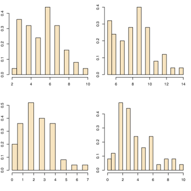
Figure 1: For $J=2$, $p_{1}=p_{2}=.5$, $q_{1\cdot}=(.2,.5,.2,.1)$, $q_{2\cdot}=(.3,.3,.1,.3)$, $\ell=20$ and $n=50$ independent simulations: histograms of the $m=4$ entries.

Another case where mixtures of Multinomial distributions occur is the latent class model where $d$ discrete variables are observed on each of $n$ individuals (Magidson and Vermunt, 2000). The observations $(1\leq i\leq n)$ are $\mathbf{x}_{i}=(x_{i1},\ldots,x_{id})$, with $x_{iv}$ taking values within the $m_{v}$ modalities of the $v$-th variable. The distribution of $\mathbf{x}_{i}$ is then

$$\sum_{j=1}^{J}p_{j}\prod_{i=1}^{d}\mathcal{M}_{m_{i}}\left(1;q_{1}^{ij},\ldots,q_{m_{i}}^{ij}\right)\,,$$

so, strictly speaking, this is a mixture of products of Multinomials. The applications of this peculiar modelling are numerous: in medical studies, it can be used to associate several symptoms or pathologies; in genetics, it may indicate that the genes corresponding to the variables are not sufficient to explain the outcome under study and that an additional (unobserved) gene may be influential. Lastly, in marketing, variables may correspond to categories of products, modalities to brands, and components of the mixture to different consumer behaviours: identifying to which group a customer belongs may help in suggesting sales, as on Web-sale sites.

Similarly, if the dominating measure is the counting measure on the set of the integers $\mathbb{N}$, the $f_{j}$’s may be Poisson distributions $\mathcal{P}(\lambda_{j})$ $(\lambda_{j}>0)$. We aim then to make inference about the parameters $(p_{j},\lambda_{j})$ from a sequence $(x_{i})_{i=1,\ldots,n}$ of integers.

The dominating measure may as well be the Lebesgue measure on $\mathbb{R}$, in which case the $f(x|\theta)$’s may all be normal distributions or Student’s $t$ distributions (or even a mix of both), with $\theta$ representing the unknown mean and variance, or the unknown mean and variance and degrees of freedom, respectively. Such a model is appropriate for datasets presenting multimodal or asymmetric features, like the aerosol dataset from Nilsson and Kulmala, (2006) presented below.

Example 2.

The estimation of particle size distribution is important in understanding the aerosol dynamics that govern aerosol formation, which is of interest in environmental and health modelling. One of the most important physical properties of aerosol particles is their size; the concentration of aerosol particles in terms of their size is referred to as the particle size distribution.

The data studied by Nilsson and Kulmala, (2006) and represented in Figure 2 is from Hyytiälä, a measurement station in Southern Finland. It corresponds to a full day of measurement, taken at ten minute intervals. $\blacktriangleleft$

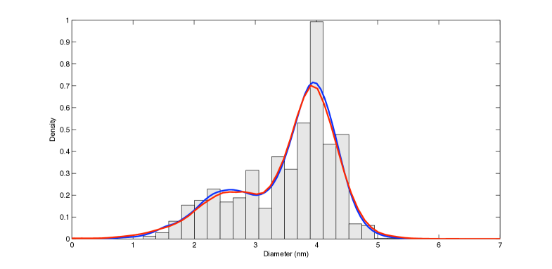
Figure 2: Histogram of the aerosol diameter dataset, along with a normal (red) and a $t$ (blue) modelling.

While the definition (1) of a mixture model is elementary, its simplicity does not extend to the derivation of either the maximum likelihood estimator (when it exists) or of Bayes estimators. In fact, if we take $n$ iid observations $\mathbf{x}=(x_{1},\ldots,x_{n})$ from (1), with parameters

$$\mathbf{p}=(p_{1}\ldots,p_{J})\quad\text{and}\quad\boldsymbol{\theta}=(\theta_{1},\ldots,\theta_{J})\,,$$

the full computation of the posterior distribution and in particular the explicit representation of the corresponding posterior expectation involves the expansion of the likelihood

$$\text{L}(\boldsymbol{\theta},\mathbf{p}|\mathbf{x})=\prod_{i=1}^{n}\sum_{j=1}^{J}p_{j}f\left(x_{i}|\theta_{j}\right)$$ (3)

into a sum of $J^{n}$ terms. with some exceptions (see, for example Section 3). This is thus computationally too expensive to be used for more than a few observations. This fundamental computational difficulty in dealing with the models (1) explains why those models have often been at the forefront for applying new technologies (such as MCMC algorithms, see Section 4).

2.2 Missing data

Mixtures of distributions are typical examples of latent variable (or missing data) models in that a sample $x_{1},\ldots,x_{n}$ from (1) can be seen as a collection of subsamples originating from each of the $f\left(x_{i}|\theta_{j}\right)$’s, when both the size and the origin of each subsample may be unknown. Thus, each of the $x_{i}$’s in the sample is a priori distributed from any of the $f_{j}$’s with probabilities $p_{j}$. Depending on the setting, the inferential goal behind this modeling may be to reconstitute the original homogeneous subsamples, sometimes called clusters, or to provide estimates of the parameters of the different components, or even to estimate the number of components.

The missing data representation of a mixture distribution can be exploited as a technical device to facilitate (numerical) estimation. By a demarginalisation argument, it is always possible to associate to a random variable $x_{i}$ from a mixture (1) a second (finite) random variable $z_{i}$ such that

$$x_{i}|z_{i}=z\sim f(x|\theta_{z})\,,\quad\mathbb{P}\left(z_{i}=j\right)=p_{j}\,.$$ (4)

This auxiliary variable $z_{i}$ identifies to which component the observation $x_{i}$ belongs. Depending on the focus of inference, the $z_{i}$’s may [or may not] be part of the quantities to be estimated. In any case, keeping in mind the availability of such variables helps into drawing inference about the “true” parameters. This is the technique behind the EM algorithm of Dempster et al., (1977) as well as the “data augmentation” algorithm of Tanner and Wong, (1987) that started MCMC algorithms.

2.3 The necessary but costly expansion of the likelihood

As noted above, the likelihood function (3) involves $J^{n}$ terms when the $n$ inner sums are expanded, that is, when all the possible values of the missing variables $z_{i}$ are taken into account. While the likelihood at a given value $\left(\boldsymbol{\theta},\mathbf{p}\right)$ can be computed in $\mathrm{O}(nJ)$ operations, the computational difficulty in using the expanded version of (3) precludes analytic solutions via maximum likelihood or Bayesian inference. Considering $n$ iid observations from model (1), if $\pi\left(\boldsymbol{\theta},\mathbf{p}\right)$ denotes the prior distribution on $\left(\boldsymbol{\theta},\mathbf{p}\right)$, the posterior distribution is naturally given by

$$\pi\left(\boldsymbol{\theta},\mathbf{p}|\mathbf{x}\right)\propto\left(\prod_{i=1}^{n}\sum_{j=1}^{J}p_{j}f\left(x_{i}|\theta_{j}\right)\right)\pi\left(\boldsymbol{\theta},\mathbf{p}\right).$$

It can therefore be computed in $\mathrm{O}(nJ)$ operations up to the normalising [marginal] constant, but, similar to the likelihood, it does not provide an intuitive distribution unless expanded.

Relying on the auxiliary variables $\mathbf{z}=\left(z_{1},\ldots,z_{n}\right)$ defined in (4), we take $\mathcal{Z}$ to be the set of all $J^{n}$ allocation vectors $\mathbf{z}$. For a given vector $\left(n_{1},\ldots,n_{J}\right)$ of the simplex $\left\{n_{1}+\ldots+n_{J}=n\right\}$, we define a subset of $\mathcal{Z}$,

$$\mathcal{Z}_{j}=\left\{\mathbf{z}:\sum_{i=1}^{n}\mathbb{I}_{z_{i}=1}=n_{1},\ldots,\sum_{i=1}^{n}\mathbb{I}_{z_{i}=J}=n_{J}\right\}\,,$$

that consists of all allocations $\mathbf{z}$ with the given allocation sizes $\left(n_{1},\ldots,n_{J}\right)$, relabelled by $j\in\mathbb{N}$ when using for instance the lexicographical ordering on $\left(n_{1},\ldots,n_{J}\right)$. The number of nonnegative integer solutions to the decomposition of $n$ into $k$ parts such that $n_{1}+\ldots+n_{J}=n$ is equal to (Feller, 1970)

$$r={n+J-1\choose n}\,.$$

Thus, we have the partition $\displaystyle\mathcal{Z}=\cup_{j=1}^{r}\mathcal{Z}_{j}$. Although the total number of elements of $\mathcal{Z}$ is the typically unmanageable $J^{n}$, the number of partition sets is much more manageable since it is of order $n^{J-1}/(J-1)!$. It is thus possible to envisage an exhaustive exploration of the $\mathcal{Z}_{j}$’s. (Casella et al., 2004 did take advantage of this decomposition to propose a more efficient important sampling approximation to the posterior distribution.)

The posterior distribution can then be written as

$$\pi\left(\boldsymbol{\theta},\mathbf{p}|\mathbf{x}\right)=\sum_{i=1}^{r}\sum_{\mathbf{z}\in\mathcal{Z}_{i}}\omega\left(\mathbf{z}\right)\pi\left(\boldsymbol{\theta},\mathbf{p}|\mathbf{x},\mathbf{z}\right)\,,$$ (5)

where $\omega\left(\mathbf{z}\right)$ represents the posterior probability of the given allocation $\mathbf{z}$. (See Section 2.4 for a derivation of $\omega\left(\mathbf{z}\right)$.) Note that with this representation, a Bayes estimator of $\left(\boldsymbol{\theta},\mathbf{p}\right)$ can be written as

$$\sum_{i=1}^{r}\sum_{\mathbf{z}\in\mathcal{Z}_{i}}\omega\left(\mathbf{z}\right)\mathbb{E}^{\pi}\left[\boldsymbol{\theta},\mathbf{p}|\mathbf{x},\mathbf{z}\right]\,.$$ (6)

This decomposition makes a lot of sense from an inferential point of view: the Bayes posterior distribution simply considers each possible allocation $\mathbf{z}$ of the dataset, allocates a posterior probability $\omega\left(\mathbf{z}\right)$ to this allocation, and then constructs a posterior distribution $\pi\left(\boldsymbol{\theta},\mathbf{p}|\mathbf{x},\mathbf{z}\right)$ for the parameters conditional on this allocation. Unfortunately, the computational burden is of order $\text{O}(J^{n})$. This is even more frustrating when considering that the overwhelming majority of the posterior probabilities $\omega\left(\mathbf{z}\right)$ will be close to zero for any sample.

2.4 Exact posterior computation

In a somewhat paradoxical twist, we now proceed to show that, in some very special cases, there exist exact derivations for the posterior distribution! This surprising phenomenon only takes place for discrete distributions under a particular choice of the component densities $f(x|\theta_{i})$. In essence, the $f(x|\theta_{i})$’s must belong to the natural exponential families, i.e.

$$f(x|\theta_{i})=h(x)\exp\left\{\theta_{i}\cdot R(x)-\Psi(\theta_{i})\right\}\,,$$

to allow for sufficient statistics to be used. In this case, there exists a conjugate prior (Robert, 2001) associated with each $\theta$ in $f(x|\theta)$ as well as for the weights of the mixture. Let us consider the complete likelihood

$$\text{L}^{c}(\boldsymbol{\theta},\mathbf{p}|\mathbf{x},\mathbf{z}) =\prod_{i=1}^{n}p_{z_{i}}\,\exp\left\{\theta_{z_{i}}\cdot R(x_{i})-\Psi(\theta_{z_{i}})\right\}$$

$$=\prod_{j=1}^{J}p_{j}^{n_{j}}\exp\left\{\theta_{j}\cdot\sum_{z_{i}=j}R(x_{i})-n_{j}\Psi(\theta_{j})\right\}$$

$$=\prod_{j=1}^{J}p_{j}^{n_{j}}\exp\left\{\theta_{j}\cdot S_{j}-n_{j}\Psi(\theta_{j})\right\}\,,$$

where $S_{j}=\sum_{z_{i}=j}R(x_{i})$. It is easily seen that we remain in an exponential family since there exist sufficient statistics with fixed dimension, $(n_{1},\ldots,n_{J},S_{1},\ldots,S_{J})$. Using a Dirichlet prior

$$\pi(p_{1},\ldots,p_{J})=\frac{\Gamma(\alpha_{1}+\ldots+\alpha_{J})}{\Gamma(\alpha_{1})\cdots\Gamma(\alpha_{J})}p_{1}^{\alpha_{1}-1}\cdots p_{J}^{\alpha_{J}-1}$$

on the vector of the weights $(p_{1},\ldots,p_{J})$ defined on the simplex of $\mathbb{R}^{J}$ and (independent) conjugate priors on the $\theta_{j}$’s,

$$\pi(\theta_{j})\propto\exp\left\{\theta_{j}\cdot\tau_{j}-\delta_{j}\Psi(\theta_{j})\right\}\,,$$

the posterior associated with the complete likelihood $\text{L}^{c}(\boldsymbol{\theta},\mathbf{p}|\mathbf{x},\mathbf{z})$ is then of the same family as the prior:

$$\pi(\boldsymbol{\theta},\mathbf{p}|\mathbf{x},\mathbf{z}) \propto\pi(\boldsymbol{\theta},\mathbf{p})\times\text{L}^{c}(\boldsymbol{\theta},\mathbf{p}|\mathbf{x},\mathbf{z})$$

$$\propto\prod_{j=1}^{J}p_{j}^{\alpha_{j}-1}\,\exp\left\{\theta_{j}\cdot\tau_{j}-\delta_{j}\Psi(\theta_{j})\right\}$$

$$\qquad\qquad\times p_{j}^{n_{j}}\exp\left\{\theta_{j}\cdot S_{j}-n_{j}\Psi(\theta_{j})\right\}$$

$$=\prod_{j=1}^{J}p_{j}^{\alpha_{j}+n_{j}-1}\,\exp\left\{\theta_{j}\cdot(\tau_{j}+S_{j})-(\delta_{j}+n_{j})\Psi(\theta_{j})\right\}\,;$$

the parameters of the prior get transformed from $\alpha_{j}$ to $\alpha_{j}+n_{j}$, from $\tau_{j}$ to $\tau_{j}+S_{j}$ and from $\delta_{j}$ to $\delta_{j}+n_{j}$.

If we now consider the observed likelihood (instead of the complete likelihood), it is the sum of the complete likelihoods over all possible configurations of the partition space of allocations, that is, a sum over $J^{n}$ terms,

$$\sum_{\mathbf{z}}\prod_{j=1}^{J}p_{j}^{n_{j}}\exp\left\{\theta_{j}\cdot S_{j}-n_{j}\Psi(\theta_{j})\right\}\,.$$

The associated posterior is then, up to a constant,

$$\sum_{\mathbf{z}} \prod_{j=1}^{J}p_{j}^{n_{j}+\alpha_{j}-1}\exp\left\{\theta_{j}\cdot(\tau_{j}+S_{j})-(n_{j}+\delta_{j})\Psi(\theta_{j})\right\}$$

$$=\sum_{\mathbf{z}}\,\omega(\mathbf{z})\,\pi(\boldsymbol{\theta},\mathbf{p}|\mathbf{x},\mathbf{z})\,,$$

where $\omega(\mathbf{z})$ is the normalising constant that is missing in

$$\prod_{j=1}^{J}p_{j}^{n_{j}+\alpha_{j}-1}\exp\left\{\theta_{j}\cdot(\tau_{j}+S_{j})-(n_{j}+\delta_{j})\Psi(\theta_{j})\right\}\,.$$

The weight $\omega(\mathbf{z})$ is therefore

$$\omega(\mathbf{z})\propto\frac{\prod_{j=1}^{J}\Gamma(n_{j}+\alpha_{j})}{\Gamma(\sum_{j=1}^{J}\{n_{j}+\alpha_{j}\})}\times\prod_{j=1}^{J}K(\tau_{j}+S_{j},n_{j}+\delta_{j})\,,$$

if $K(\tau,\delta)$ is the normalising constant of $\exp\left\{\theta_{j}\cdot\tau-\delta\Psi(\theta_{j})\right\}$, i.e.

$$K(\tau,\delta)=\int\exp\left\{\theta_{j}\cdot\tau-\delta\Psi(\theta_{j})\right\}\text{d}\theta_{j}\,.$$

Unfortunately, except for very few cases, like Poisson and Multinomial mixtures, this sum does not simplify into a smaller number of terms because there exist no summary statistics. From a Bayesian point of view, the complexity of the model is therefore truly of magnitude $\text{O}(J^{n})$.

We process here the cases of both the Poisson and Multinomial mixtures, noting that the former case was previously exhibited by Fearnhead, (2005).

Example 3.

Consider the case of a two component Poisson mixture,

$$x_{1},\ldots,x_{n}\stackrel{{\scriptstyle\text{iid}}}{{\sim}}p\,\mathcal{P}(\lambda_{1})+(1-p)\,\mathcal{P}(\lambda_{2})\,,$$

with a uniform prior on $p$ and exponential priors $\mathcal{E}xp(\tau_{1})$ and $\mathcal{E}xp(\tau_{2})$ on $\lambda_{1}$ and $\lambda_{2}$, respectively. For such a model, $S_{j}=\sum_{z_{i}=j}x_{i}$ and the normalising constant is then equal to

$$K(\tau,\delta) =\int_{-\infty}^{\infty}\exp\left\{\lambda_{j}\tau-\delta\log(\lambda_{j})\right\}\text{d}\lambda_{j}$$

$$=\int_{0}^{\infty}\lambda_{j}^{\tau-1}\,\exp\{-\delta\lambda_{j}\}\,\text{d}\lambda_{j}=\delta^{-\tau}\,\Gamma(\tau)\,.$$

The corresponding posterior is (up to the overall normalisation of the weights)

$$\sum_{\mathbf{z}}\, \frac{\displaystyle\prod_{j=1}^{2}\Gamma(n_{j}+1)\Gamma(1+S_{j})\big{/}(\tau_{j}+n_{j})^{S_{j}+1}}{\Gamma(2+\sum_{j=1}^{2}n_{j})}\,\pi(\boldsymbol{\theta},\mathbf{p}|\mathbf{x},\mathbf{z})$$

$$=\sum_{\mathbf{z}}\,\frac{\displaystyle\prod_{j=1}^{2}n_{j}!\,S_{j}!\big{/}(\tau_{j}+n_{j})^{S_{j}+1}}{(n+1)!}\,\pi(\boldsymbol{\theta},\mathbf{p}|\mathbf{x},\mathbf{z})$$

$$\propto\sum_{\mathbf{z}}\,\prod_{j=1}^{2}\frac{n_{j}!\,S_{j}!}{(\tau_{j}+n_{j})^{S_{j}+1}}\,\pi(\boldsymbol{\theta},\mathbf{p}|\mathbf{x},\mathbf{z})\,.$$

$\pi(\boldsymbol{\theta},\mathbf{p}|\mathbf{x},\mathbf{z})$ corresponds to a $\mathcal{B}(1+n_{j},1+n-n_{j})$ (Beta distribution) on $p_{j}$ and to a $\mathcal{G}(S_{j}+1,\tau_{j}+n_{j})$ (Gamma distribution) on $\delta_{j}$, $(j=1,2)$.
An important feature of this example is that the above sum does not involve all of the $2^{n}$ terms, simply because the individual terms factorise in $(n_{1},n_{2},S_{1},S_{2})$ that act like local sufficient statistics. Since $n_{2}=n-n_{1}$ and $S_{2}=\sum x_{i}-S_{1}$, the posterior only requires as many distinct terms as there are distinct values of the pair $(n_{1},S_{1})$ in the completed sample. For instance, if the sample is $(0,0,0,1,2,2,4)$, the distinct values of the pair $(n_{1},S_{1})$ are $(0,0),(1,0),(1,1),(1,2),(1,4),(2,0),\allowbreak(2,1),\allowbreak(2,2),\allowbreak(2,3),\allowbreak(2,4),(2,5),(2,6),\allowbreak\ldots,(6,5),\allowbreak(6,7),\allowbreak(6,8),\allowbreak(7,9)$. Hence there are $41$ distinct terms in the posterior, rather than $2^{8}=256$. $\blacktriangleleft$

Let $\mathbf{n}=\left(n_{1},\ldots,n_{J}\right)$ and $\mathbf{S}=\left(S_{1},\ldots,S_{J}\right)$. The problem of computing the number (or cardinal) $\mu_{n}(\mathbf{n},\mathbf{S})$ of terms in the sum with an identical statistic $(\mathbf{n},\mathbf{S})$ has been tackled by Fearnhead, (2005), who proposes a recurrent formula to compute $\mu_{n}(\mathbf{n},\mathbf{S})$ in an efficient book-keeping technique, as expressed below for a $k$ component mixture:

If $\mathbf{e}_{j}$ denotes the vector of length $J$ made of zeros everywhere except at component $j$ where it is equal to one, if

$$\mathbf{n}=(n_{1},\ldots,n_{J})\,,\quad\text{and}\quad\mathbf{n}-\mathbf{e}_{j}=(n_{1},\ldots,n_{j}-1,\ldots,n_{J})\,,$$

then

$$\mu_{1}(\mathbf{e}_{j},R\left(x_{1}\right)\mathbf{e}_{j})=1\,,\quad\forall j\in\{1,\ldots,J\}\,,\quad\text{and}\quad\mu_{n}(\mathbf{n},\mathbf{S})=\sum_{j=1}^{J}\mu_{n-1}(\mathbf{n}-\mathbf{e}_{j},\mathbf{S}-R\left(x_{n}\right)\mathbf{e}_{j})\,.$$

Example 4.

Once the $\mu_{n}(\mathbf{n},\mathbf{S})$’s are all recursively computed, the posterior can be written as

$$\sum_{(\mathbf{n},\mathbf{S})}\,\mu_{n}(\mathbf{n},\mathbf{S})\prod_{j=1}^{2}n_{j}!\,S_{j}!\big{/}(\tau_{j}+n_{j})^{S_{j}+1}\,\pi(\boldsymbol{\theta},\mathbf{p}|\mathbf{x},\mathbf{n},\mathbf{S})\,,$$

up to a constant, and the sum only depends on the possible values of the “sufficient” statistic $(\mathbf{n},\mathbf{S})$.
This closed form expression allows for a straightforward representation of the marginals. For instance, up to a constant, the marginal in $\lambda_{1}$ is given by

$$\sum_{\mathbf{z}}\, \prod_{j=1}^{2}n_{j}!\,S_{j}!\big{/}(\tau_{j}+n_{j})^{S_{j}+1}\,(n_{1}+1)^{S_{1}+1}\lambda^{S_{1}}\,\exp\{-(n_{1}+1)\lambda_{1}\}/n_{1}!$$

$$=\sum_{(\mathbf{n},\mathbf{S})}\mu_{n}(\mathbf{n},\mathbf{S})\,\prod_{j=1}^{2}n_{j}!\,S_{j}!\big{/}(\tau_{j}+n_{j})^{S_{j}+1}$$

$$\qquad\times(n_{1}+\tau_{1})^{S_{1}+1}\lambda_{1}^{S_{1}}\,\exp\{-(n_{1}+\tau_{1})\lambda_{1}\}/n_{1}!\,.$$

The marginal in $\lambda_{2}$ is

$$\sum_{(\mathbf{n},\mathbf{S})}\, \mu_{n}(\mathbf{n},\mathbf{S})\,\prod_{j=1}^{2}n_{j}!\,S_{j}!\big{/}(\tau_{j}+n_{j})^{S_{j}+1}$$

$$\qquad(n_{2}+\tau_{2})^{S_{2}+1}\lambda_{2}^{S_{2}}\,\exp\{-(n_{2}+\tau_{2})\lambda_{2}\}/n_{2}!\,,$$

again up to a constant.

Another interesting outcome of this closed form representation is that marginal densities can also be computed in closed form. The marginal distribution of $\mathbf{x}$ is directly related to the unnormalised weights in that

$$m(\mathbf{x})=\sum_{\mathbf{z}}\omega(\mathbf{z})=\sum_{(\mathbf{n},\mathbf{S})}\mu_{n}(\mathbf{n},\mathbf{S})\,\frac{\prod_{j=1}^{2}n_{j}!\,S_{j}!\big{/}(\tau_{j}+n_{j})^{S_{j}+1}}{(n+1)!}$$

up to the product of factorials $1/x_{1}!\cdots x_{n}!$ (but this product is irrelevant in the computation of the Bayes factor). $\blacktriangleleft$

Now, even with this considerable reduction in the complexity of the posterior distribution, the number of terms in the posterior still explodes fast both with $n$ and with the number of components $J$, as shown through a few simulated examples in Table 1. The computational pressure also increases with the range of the data, that is, for a given value of $(J,n)$, the number of values of the sufficient statistics is much larger when the observations are larger, as shown for instance in the first three rows of Table 1: a simulated Poisson $\mathcal{P}(\lambda)$ sample of size $10$ is mostly made of $0$’s when $\lambda=.1$ but mostly takes different values when $\lambda=10$. The impact on the number of sufficient statistics can be easily assessed when $J=4$. (Note that the simulated dataset corresponding to $(n,\lambda)=(10,.1)$ in Table 1 happens to correspond to a simulated sample made only of $0$’s, which explains the $n+1=11$ values of the sufficient statistic $(n_{1},S_{1})=(n_{1},0)$ when $J=2$.)

$(n,\lambda)$	$J=2$	$J=3$	$J=4$
$(10,.1)$	11	66	286
$(10,1)$	52	885	8160
$(10,10)$	166	7077	120,908
$(20,.1)$	57	231	1771
$(20,1)$	260	20,607	566,512
$(20,10)$	565	100,713	—
$(30,.1)$	87	4060	81,000
$(30,1)$	520	82,758	—
$(30,10)$	1413	637,020	—

Table 1: Number of pairs $(\mathbf{n},\mathbf{S})$ for simulated datasets from a Poisson $\mathcal{P}(\lambda)$ and different numbers of components. (Missing terms are due to excessive computational or storage requirements.)

Example 5.

If we have $n$ observations $\mathbf{n}_{i}=(n_{i1},\ldots,n_{im})$ from the Multinomial mixture

$$\mathbf{n}_{i}\sim p\mathcal{M}_{m}(d_{i};q_{11},\ldots,q_{1m})+(1-p)\mathcal{M}_{m}(d_{i};q_{21},\ldots,q_{2m})\,$$

where $n_{i1}+\cdots+n_{im}=d_{i}$ and $q_{11}+\cdots+q_{1m}=q_{21}+\cdots+q_{2m}=1$, the conjugate priors on the $q_{jv}$’s are Dirichlet distributions, $(j=1,2)$

$$(q_{j1},\ldots,q_{jm})\sim\mathcal{D}(\alpha_{j1},\ldots,\alpha_{jm})\,,$$

and we use once again the uniform prior on $p$. (A default choice for the $\alpha_{jv}$’s is $\alpha_{jv}=1/2$.) Note that the $d_{j}$’s may differ from observation to observation, since they are irrelevant for the posterior distribution: given a partition $\mathbf{z}$ of the sample, the complete posterior is indeed

$$p^{n_{1}}(1-p)^{n_{2}}\,\prod_{j=1}^{2}\prod_{z_{i}=j}q_{j1}^{n_{i1}}\cdots q_{jm}^{n_{im}}\,\times\prod_{j=1}^{2}\prod_{v=1}^{m}q_{jv}^{-1/2},$$

(where $n_{j}$ is the number of observations allocated to component $j$) up to a normalising constant that does not depend on $\mathbf{z}$. $\blacktriangleleft$

More generally, considering a Multinomial mixture with $m$ components,

$$\mathbf{n}_{i}\sim\sum_{j=1}^{J}p_{j}\mathcal{M}_{m}(d_{i};q_{j1},\ldots,q_{jm})\,,$$

the complete posterior is also directly available, as

$$\prod_{j=1}^{J}p_{j}^{n_{j}}\times\prod_{j=1}^{J}\prod_{z_{i}=j}q_{j1}^{n_{i1}}\cdots q_{jm}^{n_{im}}\,\times\prod_{j=1}^{J}\prod_{v=1}^{m}q_{jv}^{-1/2},$$

once more up to a normalising constant.

Since the corresponding normalising constant of the Dirichlet distribution is

$$\frac{\prod_{v=1}^{m}\Gamma(\alpha_{jv})}{\Gamma(\alpha_{j1}+\cdots+\alpha_{jm})}\,,$$

the overall weight of a given partition $\mathbf{z}$ is

$$n_{1}!n_{2}!\frac{\prod_{v=1}^{m}\Gamma(\alpha_{1v}+S_{1v})}{\Gamma(\alpha_{11}+\cdots+\alpha_{1m}+S_{1\cdot})}\times\frac{\prod_{v=1}^{m}\Gamma(\alpha_{2v}+S_{2v})}{\Gamma(\alpha_{21}+\cdots+\alpha_{2m}+S_{2\cdot})}\,$$ (7)

where $S_{ji}$ is the sum of the $n_{ji}$’s for the observations $i$ allocated to component $j$ and

$$S_{ji}=\sum_{z_{i}=j}n_{ji}\quad\text{and}\quad S_{j\cdot}=\sum_{i}S_{ji}\,.$$

Given that the posterior distribution only depends on those “sufficient” statistics $S_{ij}$ and $n_{i}$, the same factorisation as in the Poisson case applies, namely we simply need to count the number of occurrences of a particular local sufficient statistic $(n_{1},S_{11},\ldots,S_{Jm})$ and then sum over all values of this sufficient statistic. The book-keeping algorithm of Fearnhead, (2005) applies. Note however that the number of different terms in the closed form expression is growing extremely fast with the number of observations, with the number of components and with the number $k$ of modalities.

Example 6.

In the case of the latent class model, consider the simplest case of two variables with two modalities each, so observations are products of Bernoulli’s,

$$\mathbf{x}\sim p\mathcal{B}(q_{11})\mathcal{B}(q_{12})+(1-p)\mathcal{B}(q_{21})\mathcal{B}(q_{22})\,.$$

We note that the corresponding statistical model is not identifiable beyond the usual label switching issue detailled in Section 3.1. Indeed, there are only two dichotomous variables, four possible realizations for the $\mathbf{x}$’s, and five unknown parameters. We however take advantage of this artificial model to highlight the implementation of the above exact algorithm, which can then easily uncover the unidentifiability features of the posterior distribution.

The complete posterior distribution is the sum over all partitions of the terms

$$p^{n_{1}}(1-p)^{n_{2}}\,\prod_{j=1}^{2}\,\prod_{v=1}^{2}\,q_{jv}^{s_{jv}}(1-q_{jv})^{n_{j}-s_{jv}}\times\prod_{j=1}^{2}\prod_{v=1}^{2}q_{jv}^{-1/2}$$

where $s_{jv}=\sum_{z_{i}=j}x_{iv}$, the sufficient statistic is thus $(n_{1},s_{11},s_{12},s_{21},s_{22})$, of order $\text{O}(n^{5})$. Using the benchmark data of Stouffer and Toby, (1951), made of 216 sample points involving four binary variables related with a sociological questionnaire, we restricted ourselves to both first variables and 50 observations picked at random. A recursive algorithm that eliminated replicates gives the results that (a) there are $5,928$ different values for the sufficient statistic and (b) the most common occurrence is the middle partition $(26,6,11,5,10)$, with $7.16\times 10^{12}$ replicas (out of $1.12\times 10^{15}$ total partitions). The posterior weight of a given partition is

$$\frac{\Gamma(n_{1}+1)\Gamma(n-n_{1}+1)}{\Gamma(n+2)}\,\prod_{j=1}^{2}\,\prod_{v=1}^{2}\frac{\Gamma(s_{jv}+1/2)\Gamma(n_{j}-s_{jv}+1/2)}{\Gamma(n_{j}+1)}$$

$$\quad=\prod_{j=1}^{2}\,\prod_{v=1}^{2}\Gamma(s_{jv}+1/2)\Gamma(n_{j}-s_{jv}+1/2)\bigg{/}n_{1}!\,(n-n_{1})!\,(n+1)!\,,$$

multiplied by the number of occurrences. In this case, it is therefore possible to find exactly the most likely partitions, namely the one with $n_{1}=11$ and $n_{2}=39$, $s_{11}=11$, $s_{12}=8$, $s_{21}=0$, $s_{22}=17$, and the symmetric one, which both only occur once and which have a joint posterior probability of $0.018$. It is also possible to eliminate all the partitions with very low probabilities in this example. $\blacktriangleleft$

3 Mixture inference

Once again, the apparent simplicity of the mixture density should not be taken at face value for inferential purposes; since, for a sample of arbitrary size $n$ from a mixture distribution (1), there always is a non-zero probability $(1-p_{j})^{n}$ that the $j$th subsample is empty, the likelihood includes terms that do not bring any information about the parameters of the $i$-th component.

3.1 Nonidentifiability, hence label switching

A mixture model (1) is senso stricto never identifiable since it is invariant under permutations of the indices of the components. Indeed, unless we introduce some restriction on the range of the $\theta_{i}$’s, we cannot distinguish component number $1$ (i.e., $\theta_{1}$) from component number $2$ (i.e., $\theta_{2}$) in the likelihood, because they are exchangeable. This apparently benign feature has consequences on both Bayesian inference and computational implementation. First, exchangeability implies that in a $J$ component mixture, the number of modes is of order $\mathrm{O}(J!)$. The highly multimodal posterior surface is therefore difficult to explore via standard Markov chain Monte Carlo techniques. Second, if an exchangeable prior is used on $\boldsymbol{\theta}=\left(\theta_{1},\ldots,\theta_{J}\right)$, all the marginals of the $\theta_{j}$’s are identical. Other and more severe sources of unidentifiability could occur as in Example 6.

Example 7.

(Example 6 continued) If we continue our assessment of the latent class model, with two variables with two modalities each, based on subset of data extracted from Stouffer and Toby, (1951), under a Beta, $\mathcal{B}(a,b)$, prior distribution on $p$ the posterior distribution is the weighted sum of Beta $\mathcal{B}(n_{1}+a,n-n_{1}+b)$ distributions, with weights

$$\mu_{n}(\mathbf{n},\mathbf{s})\,\prod_{j=1}^{2}\,\prod_{v=1}^{2}\Gamma(s_{jv}+1/2)\Gamma(n_{j}-s_{jv}+1/2)\bigg{/}n_{1}!\,(n-n_{1})!\,(n+1)!\,,$$

where $\mu_{n}(\mathbf{n},\mathbf{s})$ denotes the number of occurrences of the sufficient statistic. Figure 3 provides the posterior distribution for a subsample of the dataset of Stouffer and Toby, (1951) and $a=b=1$. Since $p$ is not identifiable, the impact of the prior distribution is stronger than in an identifying setting: using a Beta $\mathcal{B}(a,b)$ prior on $p$ thus produces a posterior [distribution] that reflects as much the influence of $(a,b)$ as the information contained in the data. While a $\mathcal{B}(1,1)$ prior, as in Figure 3, leads to a perfectly symmetric posterior with three modes, using an assymetric prior with $a\ll b$ strongly modifies the range of the posterior, as illustrated by Figure 4. $\blacktriangleleft$

Figure 3: Exact posterior distribution of $p$ for a sample of $50$ observations from the dataset of Stouffer and Toby, (1951) and $a=b=1$.

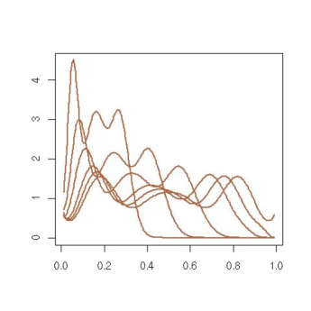
Figure 4: Exact posterior distributions of $p$ for a sample of 50 observations from the dataset of Stouffer and Toby, (1951) under Beta $\mathcal{B}(a,b)$ priors when $a=.01,.05,.1,.05,1$ and $b=100,50,20,10,5,1$.

Identifiability problems resulting from the exchangeability issue are called “label switching” in that the output of a properly converging MCMC algorithm should produce no information about the component labels (a feature which, incidentally, provides a fast assessment of the performance of MCMC solutions, as proposed in Celeux et al., 2000). A naïve answer to the problem proposed in the early literature is to impose an identifiability constraint on the parameters, for instance by ordering the means (or the variances or the weights) in a normal mixture. From a Bayesian point of view, this amounts to truncating the original prior distribution, going from $\pi\left(\boldsymbol{\theta},\mathbf{p}\right)$ to

$$\pi\left(\boldsymbol{\theta},\mathbf{p}\right)\,\mathbb{I}_{\mu_{1}\leq\ldots\leq\mu_{J}}\,.$$

While this device may seem innocuous (because indeed the sampling distribution is the same with or without this constraint on the parameter space), it is not without consequences on the resulting inference. This can be seen directly on the posterior surface: if the parameter space is reduced to its constrained part, there is no agreement between the above notation and the topology of this surface. Therefore, rather than selecting a single posterior mode and its neighbourhood, the constrained parameter space will most likely include parts of several modal regions. Thus, the resulting posterior mean may well end up in a very low probability region and be unrepresentative of the estimated distribution.

Note that, once an MCMC sample has been simulated from an unconstrained posterior distribution, any ordering constraint can be imposed on this sample, that is, after the simulations have been completed, for estimation purposes as stressed by Stephens, (1997). Therefore, the simulation (if not the estimation) hindrance created by the constraint can be completely bypassed.

Once an MCMC sample has been simulated from an unconstrained posterior distribution, a natural solution is to identify one of the $J!$ modal regions of the posterior distribution and to operate the relabelling in terms of proximity to this region, as in Marin et al., (2005). Similar approaches based on clustering algorithms for the parameter sample are proposed in Stephens, (1997) and Celeux et al., (2000), and they achieve some measure of success on the examples for which they have been tested.

3.2 Restrictions on priors

From a Bayesian point of view, the fact that few or no observation in the sample is (may be) generated from a given component has a direct and important drawback: this prohibits the use of independent improper priors,

$$\pi\left(\boldsymbol{\theta}\right)=\prod_{j=1}^{J}\pi(\theta_{j})\,,$$

since, if

$$\int\pi(\theta_{j})\hbox{d}\theta_{j}=\infty$$

then for any sample size $n$ and any sample $\mathbf{x}$,

$$\int\pi(\boldsymbol{\theta},\mathbf{p}|\mathbf{x})\hbox{d}\boldsymbol{\theta}\hbox{d}\mathbf{p}=\infty\,.$$

The ban on using improper priors can be considered by some as being of little importance, since proper priors with large variances could be used instead. However, since mixtures are ill-posed problems, this difficulty with improper priors is more of an issue, given that the influence of a particular proper prior, no matter how large its variance, cannot be truly assessed.

There exists, nonetheless, a possibility of using improper priors in this setting, as demonstrated for instance by Mengersen and Robert, (1996), by adding some degree of dependence between the component parameters. In fact, a Bayesian perspective makes it quite easy to argue against independence in mixture models, since the components are only properly defined in terms of one another. For the very reason that exchangeable priors lead to identical marginal posteriors on all components, the relevant priors must contain some degree of information that components are different and those priors must be explicit about this difference.

The proposal of Mengersen and Robert, (1996), also described in Marin et al., (2005), is to introduce first a common reference, namely a scale, location, or location-scale parameter $(\mu,\tau)$, and then to define the original parameters in terms of departure from those references. Under some conditions on the reparameterisation, expressed in Robert and Titterington, (1998), this representation allows for the use of an improper prior on the reference parameter $(\mu,\tau)$. See Wasserman, (2000), Pérez and Berger, (2002), Moreno and Liseo, (2003) for different approaches to the use of default or non-informative priors in the setting of mixtures.

4 Inference for mixtures with a known number of components

In this section, we describe different Monte Carlo algorithms that are customarily used for the approximation of posterior distributions in mixture settings when the number of components $J$ is known. We start in Section 4.1 with a proposed solution to the label-switching problem and then discuss in the following sections Gibbs sampling and Metropolis-Hastings algorithms, acknowledging that a diversity of other algorithms exist (tempering, population Monte Carlo…), see Robert and Casella, (2004).

4.1 Reordering

Section 3.1 discussed the drawbacks of imposing identifiability ordering constraints on the parameter space for estimation performances and there are similar drawbacks on the computational side, since those constraints decrease the explorative abilities of a sampler and, in the most extreme cases, may even prevent the sampler from converging (see Celeux et al., 2000). We thus consider samplers that evolve in an unconstrained parameter space, with the specific feature that the posterior surface has a number of modes that is a multiple of $J!$. Assuming that this surface is properly visited by the sampler (and this is not a trivial assumption), the derivation of point estimates of the parameters of (1) follows from an ex-post reordering proposed by Marin et al., (2005) which we describe below.

Given a simulated sample of size $M$, a starting value for a point estimate is the naïve approximation to the Maximum a Posteriori (MAP) estimator, that is the value in the sequence $(\boldsymbol{\theta},\mathbf{p})^{(l)}$ that maximises the posterior,

$$l^{*}=\arg\max_{l=1,\ldots,M}\pi((\boldsymbol{\theta},\mathbf{p})^{(l)}|\mathbf{x})$$

Once an approximated MAP is computed, it is then possible to reorder all terms in the sequence $(\boldsymbol{\theta},\mathbf{p})^{(l)}$ by selecting the reordering that is the closest to the approximate MAP estimator for a specific distance in the parameter space. This solution bypasses the identifiability problem without requiring a preliminary and most likely unnatural ordering with respect to one of the parameters (mean, weight, variance) of the model. Then, after the reordering step, an estimation of $\theta_{j}$ is given by

$$\sum_{l=1}^{M}(\theta_{j})^{(l)}\big{/}M\,.$$

4.2 Data augmentation and Gibbs sampling approximations

The Gibbs sampler is the most commonly used approach in Bayesian mixture estimation (Diebolt and Robert, 1990, 1994, Lavine and West, 1992, Verdinelli and Wasserman, 1992, Escobar and West, 1995) because it takes advantage of the missing data structure of the $z_{i}$’s uncovered in Section 2.2.

The Gibbs sampler for mixture models (1) (Diebolt and Robert, 1994) is based on the successive simulation of $\mathbf{z}$, $\mathbf{p}$ and $\boldsymbol{\theta}$ conditional on one another and on the data, using the full conditional distributions derived from the conjugate structure of the complete model. (Note that $\mathbf{p}$ only depends on the missing data $\mathbf{z}$.)

Gibbs sampling for mixture models

1. Initialization: choose $\mathbf{p}^{(0)}$ and $\boldsymbol{\theta}^{(0)}$ arbitrarily

2. Step t. For $t=1,\ldots$

   1. Generate $z_{i}^{(t)}$ ($i=1,\ldots,n$) from ($j=1,\ldots,J$)

      $\mathbb{P}\left(z_{i}^{(t)}=j|p_{j}^{(t-1)},\theta_{j}^{(t-1)},x_{i}\right)\propto p_{j}^{(t-1)}f\left(x_{i}|\theta_{j}^{(t-1)}\right)$

   2. Generate $\mathbf{p}^{(t)}$ from $\pi(\mathbf{p}|\mathbf{z}^{(t)})$

   3. Generate $\boldsymbol{\theta}^{(t)}$ from $\pi(\boldsymbol{\theta}|\mathbf{z}^{(t)},\mathbf{x})$.

As always with mixtures, the convergence of this MCMC algorithm is not as easy to assess as it seems at first sight. In fact, while the chain is uniformly geometrically ergodic from a theoretical point of view, the severe augmentation in the dimension of the chain brought by the completion stage may induce strong convergence problems. The very nature of Gibbs sampling may lead to “trapping states”, that is, concentrated local modes that require an enormous number of iterations to escape from. For example, components with a small number of allocated observations and very small variance become so tightly concentrated that there is very little probability of moving observations in or out of those components, as shown in Marin et al., (2005). As discussed in Section 2.3, Celeux et al., (2000) show that most MCMC samplers for mixtures, including the Gibbs sampler, fail to reproduce the permutation invariance of the posterior distribution, that is, that they do not visit the $J!$ replications of a given mode.

Example 8.

Consider a mixture of normal distributions with common variance $\sigma^{2}$ and unknown means and weights

$$\sum_{j=1}^{J}p_{j}\,\mathcal{N}(\mu_{j},\sigma^{2})\,.$$

This model is a particular case of model (1) and is not identifiable. Using conjugate exchangeable priors

$$\mathbf{p}\sim\mathcal{D}(1,\ldots,1)\,,\quad\mu_{j}\sim\mathcal{N}(0,10\sigma^{2})\,,\quad\sigma^{-2}\sim\mathcal{E}xp(1/2)\,,$$

it is straightforward to implement the above Gibbs sampler:

• the weight vector $\mathbf{p}$ is simulated as the Dirichlet variable

  $$\mathcal{D}(1+n_{1},\ldots,1+n_{J})\,;$$

• the inverse variance as the Gamma variable

  $$\mathcal{G}\left\{(n+2)/2,(1/2)\left[1+\sum_{j=1}^{J}\left(\frac{0.1n_{j}\bar{x}_{j}^{2}}{n_{j}+0.1}+s_{j}^{2}\right)\right]\right\}\,;$$

• and, conditionally on $\sigma$, the means $\mu_{j}$ are simulated as the Gaussian variable

  $$\mathcal{N}(n_{j}\bar{x}_{j}/(n_{j}+0.1),\sigma^{2}/(n_{j}+0.1))\,;$$

where $n_{j}=\sum_{z_{i}=j}$, $\bar{x}_{j}=\sum_{z_{i}=j}x_{i}$ and $s_{j}^{2}=\sum_{z_{i}=j}(x_{i}-\bar{x}_{j})^{2}/n_{j}$.
Note that this choice of implementation allows for the block simulation of the means-variance group, rather than the more standard simulation of the means conditional on the variance and of the variance conditional on the means (as in Diebolt and Robert, 1994). $\blacktriangleleft$

Consider the benchmark dataset of the galaxy radial speeds described for instance in Roeder and Wasserman, (1997). The output of the Gibbs sampler is summarised on Figure 5 in the case of $J=3$ components. As is obvious from the comparison of the three first histograms (and of the three following ones), label switching does not occur with this sampler: the three components remain isolated during the simulation process. $\blacktriangleleft$

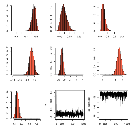
Figure 5: From the left to the right, histograms of the parameters $(p_{1},p_{2},p_{3},\mu_{1},\mu_{2},\mu_{3},\sigma)$ of a normal mixture with $k=3$ components based on $10^{4}$ iterations of the Gibbs sampler and the galaxy dataset, evolution of the $\sigma$ and of the log-likelihood.

Note that Geweke, (2007) (among others) dispute the relevance of asking for proper mixing over the $k!$ modes, arguing that on the contrary the fact that the Gibbs sampler sticks to a single mode allows for an easier inference. We obviously disagree with this perspective: first, from an algorithmic point of view, given the unconstrained posterior distribution as the target, a sampler that fails to explore all modes clearly fails to converge. Second, the idea that being restricted to a single mode provides a proper representation of the posterior is naïvely based on an intuition derived from mixtures with few components. As the number of components increases, modes on the posterior surface get inextricably mixed and a standard MCMC chain cannot be garanteed to remain within a single modal region. Furthermore, it is impossible to check in practice whether not this is the case.

In his defence of “simple” MCMC strategies supplemented with postprocessing steps, Geweke, (2007) states that

[Celeux et al.’s (2000)] argument is persuasive only to the extent that there are mixing problems beyond those arising from permutation invariance of the posterior distribution. Celeux et al. (2000) does not make this argument, indeed stating “The main defect of the Gibbs sampler from our perspective is the ultimate attraction of the local modes” (p. 959). That article produces no evidence of additional mixing problems in its examples, and we are not aware of such examples in the related literature. Indeed, the simplicity of the posterior distributions conditional on state assignments in most mixture models leads one to expect no irregularities of this kind.

There are however clear irregularities in the convergence behaviour of Gibbs and Metropolis–Hastings algorithms as exhibited in Marin et al., (2005) and Marin and Robert, (2007) (Figure 6.4) for an identifiable two-component normal mixture with both means unknown. In examples as such as those, there exist secondary modes that may have much lower posterior values than the modes of interest but that are nonetheless too attractive for the Gibbs sampler to visit other modes. In such cases, the posterior inference derived from the MCMC output is plainly incoherent. (See also Iacobucci et al., (2008) for another illustration of a multimodal posterior distribution in an identifiable mixture setting.)

However, as shown by the example below, for identifiable mixture models, there is no label switching to expect and the Gibbs sampler may work quite well. While there is no foolproof approach to check MCMC convergence (Robert and Casella, 2004), we recommend using the visited likelihoods to detect lack of mixing in the algorithms. This does not detect the label switching difficulties (but individual histograms do) but rather the possible trapping of a secondary mode or simply the slow exploration of the posterior surface. This is particularly helpful when implementing multiple runs in parallel.

Example 9.

(Example 2 continued) Consider the case of a mixture of Student’s $t$ distributions with known and different numbers of degrees of freedom

$$\sum_{j=1}^{J}p_{j}t_{\nu_{j}}(\mu_{j},\sigma_{j}^{2})\,.$$

This mixture model is not a particular case of model (1) and is identifiable. Moreover, since the noncentral $t$ distribution $t_{\nu}(\mu,\sigma^{2})$ can be interpreted as a continuous mixture of normal distributions with a common mean and with variances distributed as scaled inverse $\chi^{2}$ random variable, a Gibbs sampler can be easily implemented in this setting by taking advantage of the corresponding latent variables: $x_{i}\sim t_{\nu}(\mu,\sigma^{2})$ is the marginal of

$$x_{i}|V_{i},\sigma^{2}\sim\mathcal{N}(\mu,V_{i}\sigma^{2})\,,\qquad V_{i}^{-1}\sim\chi^{2}_{\nu}\,.$$

Once these latent variables are included in the simulation, the conditional posterior distributions of all parameters are available when using conjugate priors like

$$\mathbf{p}\sim\mathcal{D}(1,\dots,1)\,,\quad\mu_{j}\sim\mathcal{N}(\mu_{0},2\sigma_{0}^{2})\,,\quad\sigma^{2}_{j}\sim\mathcal{IG}(\alpha_{\sigma},\beta_{\sigma})\,.$$

The full conditionals for the Gibbs sampler are a Dirichlet $\mathcal{D}(1+n_{1},\dots,1+n_{J})$ distribution on the weight vector, inverse Gamma

$$\mathcal{IG}\left\{\alpha_{\sigma}+\dfrac{n_{j}}{2}~{},\beta_{\sigma}+\sum_{z_{i}=j}\dfrac{(x_{i}-\mu_{j})^{2}}{2V_{i}}\right\}$$

distributions on the variances $\sigma^{2}_{j}$, normal

$$\mathcal{N}\left(\dfrac{\mu_{0}\sigma_{j}^{2}+2\sigma_{0}^{2}\sum_{z_{i}=j}x_{i}V^{-1}_{i}}{\sigma_{j}^{2}+2\sigma_{0}^{2}\sum_{z_{i}=j}V^{-1}_{i}}~{},\dfrac{2\sigma_{0}^{2}\sigma_{j}^{2}}{\sigma_{j}^{2}+2\sigma_{0}^{2}\sum_{z_{i}=j}V^{-1}_{i}}\right)$$

distributions on the means $\mu_{j}$, and inverse Gamma

$$\mathcal{IG}\left(\dfrac{1}{2}+\dfrac{\nu_{j}}{2}~{},\dfrac{(x_{i}-\mu_{j})^{2}}{2\sigma^{2}_{j}}+\dfrac{\nu_{j}}{2}\right)$$

distributions on the $V_{i}$.

In order to illustrate the performance of the algorithm, we simulated $2,000$ observations from the two-component $t$ mixture with $\mu_{1}=0$, $\mu_{2}=5$, $\sigma^{2}_{1}=\sigma^{2}_{2}=1$, $\nu_{1}=5$, $\nu_{2}=11$ and $p_{1}=0.3$. The output of the Gibbs sampler is summarized in Figure 6. The mixing behaviour of the Gibbs chains seems to be excellent, as they explore neighbourhoods of the true values. $\blacktriangleleft$

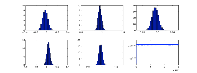
Figure 6: Histograms of the parameters, $\mu_{1},\sigma_{1},p_{1},\mu_{2},\sigma_{2}$, and evolution of the (observed) log-likelihood along $30,000$ iterations of the Gibbs sampler and a sample of $2,000$ observations.

The example below shows that, for specific models and a small number of components, the Gibbs sampler may recover the symmetry of the target distribution.

Example 10.

(Example 6 continued) For the latent class model, if we use all four variables with two modalities each in Stouffer and Toby, (1951), the Gibbs sampler involves two steps: the completion of the data with the component labels, and the simulation of the probabilities $p$ and $q_{tj}$ from Beta $\mathcal{(}B)(s_{tj}+.5,n_{j}-s_{tj}+.5)$ conditional distributions. For the $216$ observations, the Gibbs sampler seems to converge satisfactorily since the output in Figure 7 exhibits the perfect symmetry predicted by the theory. We can note that, in this special case, the modes are well separated, and hence values can be crudely estimated for $q_{1j}$ by a simple graphical identification of the modes. $\blacktriangleleft$

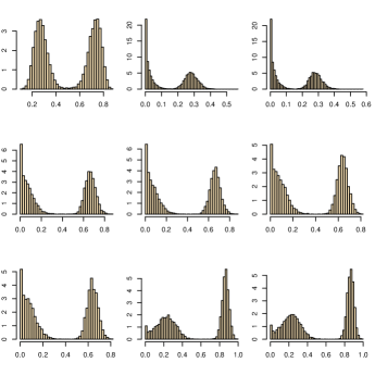
Figure 7: Latent class model: histograms of $p$ and of the $q_{tj}$’s for $10^{4}$ iterations of the Gibbs sampler and the four variables of Stouffer and Toby, (1951). The first histogram corresponds to $p$, the next on the right to $q_{11}$, followed by $q_{21}$ (identical), then $q_{21}$, $q_{22}$, and so on.

4.3 Metropolis–Hastings approximations

The Gibbs sampler may fail to escape the attraction of a local mode, even in a well-behaved case as in Example 1 where the likelihood and the posterior distributions are bounded and where the parameters are identifiable. Part of the difficulty is due to the completion scheme that increases the dimension of the simulation space and that reduces considerably the mobility of the parameter chain. A standard alternative that does not require completion and an increase in the dimension is the Metropolis–Hastings algorithm. In fact, the likelihood of mixture models is available in closed form, being computable in O$(Jn)$ time, and the posterior distribution is thus available up to a multiplicative constant.

General Metropolis–Hastings algorithm for mixture models

1. Initialization. Choose $\mathbf{p}^{(0)}$ and $\boldsymbol{\theta}^{(0)}$

2. Step t. For $t=1,\ldots$

   1. Generate $(\widetilde{\boldsymbol{\theta}},\widetilde{\mathbf{p}})$ from $q\left(\boldsymbol{\theta},\mathbf{p}|\boldsymbol{\theta}^{(t-1)},\mathbf{p}^{(t-1)}\right)$,

   2. Compute

      $$r=\frac{f(\mathbf{x}|\widetilde{\boldsymbol{\theta}},\widetilde{\mathbf{p}})\pi(\widetilde{\boldsymbol{\theta}},\widetilde{\mathbf{p}})q(\boldsymbol{\theta}^{(t-1)},\mathbf{p}^{(t-1)}|\widetilde{\boldsymbol{\theta}},\widetilde{\mathbf{p}})}{f(\mathbf{x}|\boldsymbol{\theta}^{(t-1)},\mathbf{p}^{(t-1)})\pi(\boldsymbol{\theta}^{(t-1)},\mathbf{p}^{(t-1)})q(\widetilde{\boldsymbol{\theta}},\widetilde{\mathbf{p}}|\boldsymbol{\theta}^{(t-1)},\mathbf{p}^{(t-1)})},$$

   3. Generate $u\sim\mathscr{U}_{[0,1]}$
      If $r>u$ then $(\boldsymbol{\theta}^{(t)},\mathbf{p}^{(t)})=(\widetilde{\boldsymbol{\theta}},\widetilde{\mathbf{p}})$
      else $(\boldsymbol{\theta}^{(t)},\mathbf{p}^{(t)})=(\boldsymbol{\theta}^{(t-1)},\mathbf{p}^{(t-1)})$.

The major difference with the Gibbs sampler is that we need to choose the proposal distribution $q$, which can be a priori anything, and this is a mixed blessing! The most generic proposal is the random walk Metropolis–Hastings algorithm where each unconstrained parameter is the mean of the proposal distribution for the new value, that is,

$$\widetilde{\theta_{j}}=\theta_{j}^{(t-1)}+u_{j}$$

where $u_{j}\sim\mathcal{N}(0,\zeta^{2})$. However, for constrained parameters like the weights and the variances in a normal mixture model, this proposal is not efficient.

This is indeed the case for the parameter $\mathbf{p}$, due to the constraint that $\sum_{j=1}^{J}p_{j}\allowbreak=1$. To solve this difficulty, Cappé et al., (2003) propose to overparameterise the model (1) as

$$p_{j}={w_{j}}\bigg{/}{\displaystyle\sum_{l=1}^{J}w_{l}}\,,\quad w_{j}>0\,,$$

thus removing the simulation constraint on the $p_{j}$’s. Obviously, the $w_{j}$’s are not identifiable, but this is not a difficulty from a simulation point of view and the $p_{j}$’s remain identifiable (up to a permutation of indices). Perhaps paradoxically, using overparameterised representations often helps with the mixing of the corresponding MCMC algorithms since they are less constrained by the dataset or the likelihood. The proposed move on the $w_{j}$’s is $\log(\widetilde{w_{j}})=\log(w_{j}^{(t-1)})+u_{j}$ where $u_{j}\sim\mathcal{N}(0,\zeta^{2})$.

Example 11.

(Example 2 continued) We now consider the more realistic case when the degrees of freedom of the $t$ distributions are unknown. The Gibbs sampler cannot be implemented as such given that the distribution of the $\nu_{j}$’s is far from standard. A common alternative (Robert and Casella, 2004) is to introduce a Metropolis step within the Gibbs sampler to overcome this difficulty. If we use the same Gamma prior distribution with hyperparameters $(\alpha_{\nu},\beta_{\nu})$ for all the $\nu_{j}$s, the full conditional density of $\nu_{j}$ is

$$\pi(\nu_{j}|\mathbf{V},\mathbf{z})\propto\left(\dfrac{(\nu_{j}/2)^{\nu_{j}/2}}{\Gamma(\nu_{j}/2)}\right)^{n_{j}}\prod_{z_{i}=j}\dfrac{V_{i}^{-(\nu_{j}/2+1)}}{e^{\nu_{j}/2V_{i}}}\mathcal{G}(\alpha_{\nu},\beta_{\nu})\,.$$

Therefore, we resort to a random walk proposal on the $\log(\nu_{j})$’s with scale $\varsigma=5$. (The hyperparameters are $\alpha_{\nu}=5$ and $\beta_{\nu}=2$.)

In order to illustrate the performances of the algorithm, two cases are considered: (i) all parameters except variances ($\sigma^{2}_{1}=\sigma^{2}_{2}=1$) are unknown and (ii) all parameters are unknown. For a simulated dataset, the results are given on Figure 8 and Figure 9, respectively. In both cases, the posterior distributions of the $\nu_{j}$’s exhibit very large variances, which indicates that the data is very weakly informative about the degrees of freedom. The Gibbs sampler does not mix well-enough to recover the symmetry in the marginal approximations. The comparison between the estimated densities for both cases with the setting is given in Figure 10. The estimated mixture densities are indistinguishable and the fit to the simulated dataset is quite adequate. Clearly, the corresponding Gibbs samplers have recovered correctly one and only one of the $2$ symetric modes.

Figure 8: Histograms of the parameters $\mu_{1},\nu_{1},p_{1},\mu_{2},\nu_{2}$ when the variance parameters are known, and evolution of the log-likelihood for a simulated $t$ mixture with $2,000$ points, based on $3\times 10^{4}$ MCMC iterations.

Figure 9: Histograms of the parameters $\mu_{1},\sigma_{1},\nu_{1},p_{1},\mu_{2},\sigma_{2},\nu_{2}$, and evolution of the log-likelihood for a simulated $t$ mixture with $2,000$ points, based on $3\times 10^{4}$ MCMC iterations.

Figure 10: Histogram of the simulated dataset, compared with estimated $t$ mixtures with known $\sigma^{2}$ (red), known $\nu$ (green), and when all parameters are unknown (blue).

We now consider the aerosol particle dataset described in Example 2. We use the same prior distributions on the $\nu_{j}$’s as before, that is $\mathcal{G}(5,2)$. Figure 11 summarises the output of the MCMC algorithm. Since there is no label switching and only two components, we choose to estimate the parameters by the empirical averages, as illustrated in Table 2. As shown by Figure 2, both $t$ mixtures and normal mixtures fit the aerosol data reasonably well. $\blacktriangleleft$

Figure 11: Histograms of parameters ($\mu_{1},\sigma_{1},\nu_{1},p_{1},\mu_{1},\sigma_{2},\nu_{2}$) and log-likelihood of a mixture of $t$ distributions based on $30,000$ iterations and the aerosol data.

	$\mu_{1}$	$\mu_{2}$	$\sigma_{1}$	$\sigma_{2}$	$\nu_{1}$	$\nu_{2}$	$p_{1}$
Student	2.5624	3.9918	0.5795	0.3595	18.5736	19.3001	0.3336
Normal	2.5729	3.9680	0.6004	0.3704	-	-	0.3391

Table 2: Estimates of the parameters for the aerosol dataset compared for $t$ and normal mixtures.

5 Inference for mixture models with an unknown number of components

Estimation of $J$, the number of components in (1), is a special type of model choice problem, for which there is a number of possible solutions:

1. direct computation of the Bayes factors (Kass and Raftery, 1995, Chib, 1995);

2. evaluation of an entropy distance (Mengersen and Robert, 1996, Sahu and Cheng, 2003);

3. generation from a joint distribution across models via reversible jump MCMC (Richardson and Green, 1997) or via birth-and-death processes (Stephens, 2000) ;

depending on whether the perspective is on testing or estimation. We refer to Marin et al., (2005) for a short description of the reversible jump MCMC solution, a longer survey being available in Robert and Casella, (2004) and a specific description for mixtures–including an R package—being provided in Marin and Robert, (2007). The alternative birth-and-death processes proposed in Stephens, (2000) has not generated as much follow-up, except for Cappé et al., (2003) who showed that the essential mechanism in this approach was the same as with reversible jump MCMC algorithms.

We focus here on the first two approaches, because, first, the description of reversible jump MCMC algorithms require much care and therefore more space than we can allow to this paper and, second, this description exemplifies recent advances in the derivation of Bayes factors. These solutions pertain more strongly to the testing perspective, the entropy distance approach being based on the Kullback–Leibler divergence between a $J$ component mixture and its projection on the set of $J-1$ mixtures, in the same spirit as in Dupuis and Robert, (2003). Given that the calibration of the Kullback divergence is open to various interpretations (Mengersen and Robert, 1996, Goutis and Robert, 1998, Dupuis and Robert, 2003), we will only cover here some proposals regarding approximations of the Bayes factor oriented towards the direct exploitation of outputs from single model MCMC runs.

In fact, the major difference between approximations of Bayes factors based on those outputs and approximations based on the output from the reversible jump chains is that the latter requires a sufficiently efficient choice of proposals to move around models, which can be difficult despite significant recent advances (Brooks et al., 2003). If we can instead concentrate the simulation effort on single models, the complexity of the algorithm decreases (a lot) and there exist ways to evaluate the performance of the corresponding MCMC samples. In addition, it is often the case that few models are in competition when estimating $J$ and it is therefore possible to visit the whole range of potentials models in an exhaustive manner.

We have

$$f_{J}(\mathbf{x}|\boldsymbol{\lambda}_{J})=\prod_{i=1}^{n}\sum_{j=1}^{J}p_{j}f(x_{i}|\theta_{j})$$

where $\boldsymbol{\lambda}_{J}=\left(\boldsymbol{\theta},\boldsymbol{p}\right)=\left(\theta_{1},\ldots,\theta_{J},p_{1},\ldots,p_{J}\right)$. Most solutions (see, e.g. Frühwirth-Schnatter, 2006, Section 5.4) revolve around an importance sampling approximation to the marginal likelihood integral

$$m_{J}(x)=\int f_{J}(\mathbf{x}|\boldsymbol{\lambda}_{J})\,\pi_{J}(\boldsymbol{\lambda}_{J})\,\text{d}\boldsymbol{\lambda}_{J}$$

where $J$ denotes the model index (that is the number of components in the present case). For instance, Liang and Wong, (2001) use bridge sampling with simulated annealing scenarios to overcome the label switching problem. Steele et al., (2006) rely on defensive sampling and the use of conjugate priors to reduce the integration to the space of latent variables (as in Casella et al., 2004) with an iterative construction of the importance function. Frühwirth-Schnatter, (2004) also centers her approximation of the marginal likelihood on a bridge sampling strategy, with particular attention paid to identifiability constraints. A different possibility is to use Gelfand and Dey, (1994) representation: starting from an arbitrary density $g_{J}$, the equality

$$1 =\int g_{J}(\boldsymbol{\lambda}_{J})\,\text{d}\boldsymbol{\lambda}_{J}=\int\frac{g_{J}(\boldsymbol{\lambda}_{J})}{f_{J}(\mathbf{x}|\boldsymbol{\lambda}_{J})\,\pi_{J}(\boldsymbol{\lambda}_{J})}f_{J}(\mathbf{x}|\boldsymbol{\lambda}_{J})\,\pi_{J}(\boldsymbol{\lambda}_{J})\,\text{d}\boldsymbol{\lambda}_{J}$$

$$=m_{J}(\mathbf{x})\int\frac{g_{J}(\boldsymbol{\lambda}_{J})}{f_{J}(\mathbf{x}|\boldsymbol{\lambda}_{J})\,\pi_{J}(\boldsymbol{\lambda}_{J})}\pi_{J}(\boldsymbol{\lambda}_{J}|\mathbf{x})\,\text{d}\boldsymbol{\lambda}_{J}$$

implies that a potential estimate of $m_{J}(\mathbf{x})$ is

$$\hat{m}_{J}(\mathbf{x})=1\bigg{/}\frac{1}{T}\sum_{t=1}^{T}\frac{g_{J}(\boldsymbol{\lambda}_{J}^{(t)})}{f_{J}(\mathbf{x}|\boldsymbol{\lambda}_{J}^{(t)})\,\pi_{J}(\boldsymbol{\lambda}_{J}^{(t)})}$$

when the $\boldsymbol{\lambda}_{J}^{(t)}$’s are produced by a Monte Carlo or an MCMC sampler targeted at $\pi_{J}(\boldsymbol{\lambda}_{J}|\mathbf{x})$. While this solution can be easily implemented in low dimensional settings (Chopin and Robert, 2007), calibrating the auxiliary density $g_{k}$ is always an issue. The auxiliary density could be selected as a non-parametric estimate of $\pi_{k}(\boldsymbol{\lambda}_{J}|x)$ based on the sample itself but this is very costly. Another difficulty is that the estimate may have an infinite variance and thus be too variable to be trustworthy, as experimented by Frühwirth-Schnatter, (2004).

Yet another approximation to the integral $m_{J}(\mathbf{x})$ is to consider it as the expectation of $f_{J}(\mathbf{x}|\boldsymbol{\lambda}_{J})$, when $\boldsymbol{\lambda}_{J}$ is distributed from the prior. While a brute force approach simulating $\boldsymbol{\lambda}_{J}$ from the prior distribution is requiring a huge number of simulations (Neal, 1999), a Riemann based alternative is proposed by Skilling, (2006) under the denomination of nested sampling; however, Chopin and Robert, (2007) have shown in the case of mixtures that this technique could lead to uncertainties about the quality of the approximation.

We consider here a further solution, first proposed by Chib, (1995), that is straightforward to implement in the setting of mixtures (see Chib and Jeliazkov, 2001 for extensions). Although it came under criticism by Neal, (1999) (see also Frühwirth-Schnatter, 2004), we show below how the drawback pointed by the latter can easily be removed. Chib’s (1995) method is directly based on the expression of the marginal distribution (loosely called marginal likelihood in this section) in Bayes’ theorem:

$$m_{J}(\mathbf{x})=\frac{f_{J}(\mathbf{x}|\boldsymbol{\lambda}_{J})\,\pi_{J}(\boldsymbol{\lambda}_{J})}{\pi_{J}(\boldsymbol{\lambda}_{J}|\mathbf{x})}$$

and on the property that the rhs of this equation is constant in $\boldsymbol{\lambda}_{J}$. Therefore, if an arbitrary value of $\boldsymbol{\lambda}_{J}$, $\boldsymbol{\lambda}_{J}^{*}$ say, is selected and if a good approximation to $\pi_{J}(\boldsymbol{\lambda}_{J}|\mathbf{x})$ can be constructed, $\hat{\pi}_{J}(\boldsymbol{\lambda}_{J}|\mathbf{x})$, Chib’s (1995) approximation to the marginal likelihood is

$$\hat{m}_{J}(\mathbf{x})=\frac{f_{J}(\mathbf{x}|\boldsymbol{\lambda}_{J}^{*})\,\pi_{J}(\boldsymbol{\lambda}_{J}^{*})}{\hat{\pi}_{J}(\boldsymbol{\lambda}_{J}^{*}|\mathbf{x})}\,.$$ (8)

In the case of mixtures, a natural approximation to $\pi_{J}(\boldsymbol{\lambda}_{J}|\mathbf{x})$ is the Rao-Blackwell estimate

$$\hat{\pi}_{J}(\boldsymbol{\lambda}_{J}^{*}|\mathbf{x})=\frac{1}{T}\,\sum_{t=1}^{T}\pi_{J}(\boldsymbol{\lambda}_{J}^{*}|\mathbf{x},\mathbf{z}^{(t)})\,,$$

where the $\mathbf{z}^{(t)}$’s are the latent variables simulated by the MCMC sampler. To be efficient, this method requires

• a good choice of $\boldsymbol{\lambda}_{J}^{*}$ but, since in the case of mixtures, the likelihood is computable, $\boldsymbol{\lambda}_{J}^{*}$ can be chosen as the MCMC approximation to the MAP estimator and,

• a good approximation to $\pi_{J}(\boldsymbol{\lambda}_{J}|\mathbf{x})$.

This later requirement is the core of Neal’s (1999) criticism: while, at a formal level, $\hat{\pi}_{J}(\boldsymbol{\lambda}_{J}^{*}|\mathbf{x})$ is a converging (parametric) approximation to $\pi_{J}(\boldsymbol{\lambda}_{J}|\mathbf{x})$ by virtue of the ergodic theorem, this obviously requires the chain $(\mathbf{z}^{(t)})$ to converge to its stationarity distribution. Unfortunately, as discussed previously, in the case of mixtures, the Gibbs sampler rarely converges because of the label switching phenomenon described in Section 3.1, so the approximation $\hat{\pi}_{J}(\boldsymbol{\lambda}_{J}^{*}|\mathbf{x})$ is untrustworthy. Neal, (1999) demonstrated via a numerical experiment that (8) is significantly different from the true value $m_{J}(\mathbf{x})$ when label switching does not occur. There is, however, a fix to this problem, also explored by Berkhof et al., (2003), which is to recover the label switching symmetry a posteriori, replacing $\hat{\pi}_{J}(\boldsymbol{\lambda}_{J}^{*}|\mathbf{x})$ in (8) above with

$$\hat{\pi}_{J}(\boldsymbol{\lambda}_{J}^{*}|\mathbf{x})=\frac{1}{T\,J!}\,\sum_{\sigma\in\mathfrak{S}_{J}}\sum_{t=1}^{T}\pi_{J}(\sigma(\boldsymbol{\lambda}_{J}^{*})|\mathbf{x},\mathbf{z}^{(t)})\,,$$

where $\mathfrak{S}_{J}$ denotes the set of all permutations of $\{1,\ldots,J\}$ and $\sigma(\boldsymbol{\lambda}_{J}^{*})$ denotes the transform of $\boldsymbol{\lambda}_{J}^{*}$ where components are switched according to the permutation $\sigma$. Note that the permutation can equally be applied to $\boldsymbol{\lambda}_{J}^{*}$ or to the $\mathbf{z}^{(t)}$’s but that the former is usually more efficient from a computational point of view given that the sufficient statistics only have to be computed once. The justification for this modification either stems from a Rao-Blackwellisation argument, namely that the permutations are ancillary for the problem and should be integrated out, or follows from the general framework of Kong et al., (2003) where symmetries in the dominating measure should be exploited towards the improvement of the variance of Monte Carlo estimators.

Example 12.

(Example 8 continued) In the case of the normal mixture case and the galaxy dataset, using Gibbs sampling, label switching does not occur. If we compute $\log\hat{m}_{J}(\mathbf{x})$ using only the original estimate of Chib, (1995) (8), the [logarithm of the] estimated marginal likelihood is $\hat{\rho}_{J}(\mathbf{x})=-105.1396$ for $J=3$ (based on $10^{3}$ simulations), while introducing the permutations leads to $\hat{\rho}_{J}(\mathbf{x})=-103.3479$. As already noted by Neal, (1999), the difference between the original Chib’s (1995) approximation and the true marginal likelihood is close to $\log(J!)$ (only) when the Gibbs sampler remains concentrated around a single mode of the posterior distribution. In the current case, we have that $-116.3747+\log(2!)=-115.6816$ exactly! (We also checked this numerical value against a brute-force estimate obtained by simulating from the prior and averaging the likelihood, up to fourth digit agreement.) A similar result holds for $J=3$, with $-105.1396+\log(3!)=-103.3479$. Both Neal, (1999) and Frühwirth-Schnatter, (2004) also pointed out that the $\log(J!)$ difference was unlikely to hold for larger values of $J$ as the modes became less separated on the posterior surface and thus the Gibbs sampler was more likely to explore incompletely several modes. For $J=4$, we get for instance that the original Chib’s (1995) approximation is $-104.1936$, while the average over permutations gives $-102.6642$. Similarly, for $J=5$, the difference between $-103.91$ and $-101.93$ is less than $\log(5!)$. The $\log(J!)$ difference cannot therefore be used as a direct correction for Chib’s (1995) approximation because of this difficulty in controlling the amount of overlap. However, it is unnecessary since using the permutation average resolves the difficulty. Table 3 shows that the prefered value of $J$ for the galaxy dataset and the current choice of prior distribution is $J=5$. $\blacktriangleleft$

J	2	3	4	5	6	7	8
$\hat{\rho}_{J}(\mathbf{x})$	-115.68	-103.35	-102.66	-101.93	-102.88	-105.48	-108.44

Table 3: Estimations of the marginal likelihoods by the symmetrised Chib’s approximation (based on $10^{5}$ Gibbs iterations and, for $J>5$, $100$ permutations selected at random in $\mathfrak{S}_{J}$).

When the number of components $J$ grows too large for all permutations in $\mathfrak{S}_{J}$ to be considered in the average, a (random) subsample of permutations can be simulated to keep the computing time to a reasonable level when keeping the identity as one of the permutations, as in Table 3 for $J=6,7$. (See Berkhof et al., 2003 for another solution.) Note also that the discrepancy between the original Chib’s (1995) approximation and the average over permutations is a good indicator of the mixing properties of the Markov chain, if a further convergence indicator is requested.

Example 13.

(Example 6 continued) For instance, in the setting of Example 6 with $a=b=1$, both the approximation of Chib, (1995) and the symmetrized one are identical. When comparing a single class model with a two class model, the corresponding (log-)marginals are

$$\hat{\rho}_{1}(\mathbf{x})=\prod_{i=1}^{4}\frac{\Gamma(1)}{\Gamma(1/2)^{2}}\,\frac{\Gamma(n_{i}+1/2)\Gamma(n-n_{i}+1/2)}{\Gamma(n+1)}=-552.0402$$

and $\hat{\rho}_{2}(\mathbf{x})\approx-523.2978$, giving a clear preference to the two class model. $\blacktriangleleft$

References

- Berkhof et al., (2003) Berkhof, J., van Mechelen, I., and Gelman, A. (2003). A Bayesian approach to the selection and testing of mixture models. Statistica Sinica, 13:423–442.
- Brooks et al., (2003) Brooks, S., Giudici, P., and Roberts, G. (2003). Efficient construction of reversible jump Markov chain Monte Carlo proposal distributions (with discussion). J. Royal Statist. Society Series B, 65(1):3–55.
- Cappé et al., (2003) Cappé, O., Robert, C., and Rydén, T. (2003). Reversible jump, birth-and-death, and more general continuous time MCMC samplers. J. Royal Statist. Society Series B, 65(3):679–700.
- Casella et al., (2004) Casella, G., Robert, C., and Wells, M. (2004). Mixture models, latent variables and partitioned importance sampling. Statistical Methodology, 1:1–18.
- Celeux et al., (2000) Celeux, G., Hurn, M., and Robert, C. (2000). Computational and inferential difficulties with mixtures posterior distribution. J. American Statist. Assoc., 95(3):957–979.
- Chib, (1995) Chib, S. (1995). Marginal likelihood from the Gibbs output. J. American Statist. Assoc., 90:1313–1321.
- Chib and Jeliazkov, (2001) Chib, S. and Jeliazkov, I. (2001). Marginal likelihood from the Metropolis–Hastings output. J. American Statist. Assoc., 96:270–281.
- Chopin and Robert, (2007) Chopin, N. and Robert, C. (2007). Contemplating evidence: properties, extensions of, and alternatives to nested sampling. Technical Report 2007-46, CEREMADE, Université Paris Dauphine. arXiv:0801.3887.
- Dempster et al., (1977) Dempster, A., Laird, N., and Rubin, D. (1977). Maximum likelihood from incomplete data via the EM algorithm (with discussion). J. Royal Statist. Society Series B, 39:1–38.
- Diebolt and Robert, (1990) Diebolt, J. and Robert, C. (1990). Bayesian estimation of finite mixture distributions, Part i: Theoretical aspects. Technical Report 110, LSTA, Université Paris VI, Paris.
- Diebolt and Robert, (1994) Diebolt, J. and Robert, C. (1994). Estimation of finite mixture distributions by Bayesian sampling. J. Royal Statist. Society Series B, 56:363–375.
- Dupuis and Robert, (2003) Dupuis, J. and Robert, C. (2003). Model choice in qualitative regression models. J. Statistical Planning and Inference, 111:77–94.
- Escobar and West, (1995) Escobar, M. and West, M. (1995). Bayesian prediction and density estimation. J. American Statist. Assoc., 90:577–588.
- Fearnhead, (2005) Fearnhead, P. (2005). Direct simulation for discrete mixture distributions. Statistics and Computing, 15:125–133.
- Feller, (1970) Feller, W. (1970). An Introduction to Probability Theory and its Applications, volume 1. John Wiley, New York.
- Frühwirth-Schnatter, (2004) Frühwirth-Schnatter, S. (2004). Estimating marginal likelihoods for mixture and Markov switching models using bridge sampling techniques. The Econometrics Journal, 7(1):143–167.
- Frühwirth-Schnatter, (2006) Frühwirth-Schnatter, S. (2006). Finite Mixture and Markov Switching Models. Springer-Verlag, New York, New York.
- Gelfand and Dey, (1994) Gelfand, A. and Dey, D. (1994). Bayesian model choice: asymptotics and exact calculations. J. Royal Statist. Society Series B, 56:501–514.
- Geweke, (2007) Geweke, J. (2007). Interpretation and inference in mixture models: Simple MCMC works. Comput. Statist. Data Analysis. (To appear).
- Goutis and Robert, (1998) Goutis, C. and Robert, C. (1998). Model choice in generalized linear models: a Bayesian approach via Kullback–Leibler projections. Biometrika, 85:29–37.
- Iacobucci et al., (2008) Iacobucci, A., Marin, J.-M., and Robert, C. (2008). On variance stabilisation by double Rao-Blackwellisation. Technical report, CEREMADE, Université Paris Dauphine.
- Kass and Raftery, (1995) Kass, R. and Raftery, A. (1995). Bayes factors. J. American Statist. Assoc., 90:773–795.
- Kong et al., (2003) Kong, A., McCullagh, P., Meng, X.-L., Nicolae, D., and Tan, Z. (2003). A theory of statistical models for Monte Carlo integration. J. Royal Statist. Society Series B, 65(3):585–618. (With discussion.).
- Lavine and West, (1992) Lavine, M. and West, M. (1992). A Bayesian method for classification and discrimination. Canad. J. Statist., 20:451–461.
- Liang and Wong, (2001) Liang, F. and Wong, W. (2001). Real-parameter evolutionary Monte Carlo with applications to Bayesian mixture models. J. American Statist. Assoc., 96(454):653–666.
- MacLachlan and Peel, (2000) MacLachlan, G. and Peel, D. (2000). Finite Mixture Models. John Wiley, New York.
- Magidson and Vermunt, (2000) Magidson, J. and Vermunt, J. (2000). Latent class analysis. In Kaplan, D., editor, The Sage Handbook of Quantitative Methodology for the Social Sciences, pages 175–198, Thousand Oakes. Sage Publications.
- Marin et al., (2005) Marin, J.-M., Mengersen, K., and Robert, C. (2005). Bayesian modelling and inference on mixtures of distributions. In Rao, C. and Dey, D., editors, Handbook of Statistics, volume 25. Springer-Verlag, New York.
- Marin and Robert, (2007) Marin, J.-M. and Robert, C. (2007). Bayesian Core. Springer-Verlag, New York.
- Mengersen and Robert, (1996) Mengersen, K. and Robert, C. (1996). Testing for mixtures: A Bayesian entropic approach (with discussion). In Berger, J., Bernardo, J., Dawid, A., Lindley, D., and Smith, A., editors, Bayesian Statistics 5, pages 255–276. Oxford University Press, Oxford.
- Moreno and Liseo, (2003) Moreno, E. and Liseo, B. (2003). A default Bayesian test for the number of components in a mixture. J. Statist. Plann. Inference, 111(1-2):129–142.
- Neal, (1999) Neal, R. (1999). Erroneous results in “Marginal likelihood from the Gibbs output”. Technical report, University of Toronto.
- Nilsson and Kulmala, (2006) Nilsson, E. D. and Kulmala, M. (2006). Aerosol formation over the Boreal forest in Hyytiälä, Finland: monthly frequency and annual cycles - the roles of air mass characteristics and synoptic scale meteorology. Atmospheric Chemistry and Physics Discussions, 6:10425–10462.
- Pérez and Berger, (2002) Pérez, J. and Berger, J. (2002). Expected-posterior prior distributions for model selection. Biometrika, 89(3):491–512.
- Richardson and Green, (1997) Richardson, S. and Green, P. (1997). On Bayesian analysis of mixtures with an unknown number of components (with discussion). J. Royal Statist. Society Series B, 59:731–792.
- Robert, (2001) Robert, C. (2001). The Bayesian Choice. Springer-Verlag, New York, second edition.
- Robert and Casella, (2004) Robert, C. and Casella, G. (2004). Monte Carlo Statistical Methods. Springer-Verlag, New York, second edition.
- Robert and Titterington, (1998) Robert, C. and Titterington, M. (1998). Reparameterisation strategies for hidden Markov models and Bayesian approaches to maximum likelihood estimation. Statistics and Computing, 8(2):145–158.
- Roeder and Wasserman, (1997) Roeder, K. and Wasserman, L. (1997). Practical Bayesian density estimation using mixtures of normals. J. American Statist. Assoc., 92:894–902.
- Sahu and Cheng, (2003) Sahu, S. and Cheng, R. (2003). A fast distance based approach for determining the number of components in mixtures. Canadian J. Statistics, 31:3–22.
- Skilling, (2006) Skilling, J. (2006). Nested sampling for general Bayesian computation. Bayesian Analysis, 1(4):833–860.
- Steele et al., (2006) Steele, R., Raftery, A., and Emond, M. (2006). Computing normalizing constants for finite mixture models via incremental mixture importance sampling (IMIS). Journal of Computational and Graphical Statistics, 15:712–734.
- Stephens, (1997) Stephens, M. (1997). Bayesian Methods for Mixtures of Normal Distributions. PhD thesis, University of Oxford.
- Stephens, (2000) Stephens, M. (2000). Bayesian analysis of mixture models with an unknown number of components—an alternative to reversible jump methods. Ann. Statist., 28:40–74.
- Stouffer and Toby, (1951) Stouffer, S. and Toby, J. (1951). Role conflict and personality. American Journal of Sociology, 56:395–406.
- Tanner and Wong, (1987) Tanner, M. and Wong, W. (1987). The calculation of posterior distributions by data augmentation. J. American Statist. Assoc., 82:528–550.
- Verdinelli and Wasserman, (1992) Verdinelli, I. and Wasserman, L. (1992). Bayesian analysis of outliers problems using the Gibbs sampler. Statist. Comput., 1:105–117.
- Wasserman, (2000) Wasserman, L. (2000). Asymptotic inference for mixture models using data dependent priors. J. Royal Statist. Society Series B, 62:159–180.