Fractional dynamics in the Lévy quantum kicked rotor

Abstract

We investigate the quantum kicked rotor in resonance subjected to momentum measurements with a Lévy waiting time distribution. We find that the system has a sub-ballistic behavior. We obtain an analytical expression for the exponent of the power law of the variance as a function of the characteristic parameter of the Lévy distribution and connect this anomalous diffusion with a fractional dynamics.

I Introduction

During the last decades it has been possible to obtain samples of atoms at temperatures in the nano-kelvin range Cohen (optical molasses) using resonant or quasi-resonant exchanges of momentum and energy between atoms and laser light. This spectacular experimental progress has been accompanied with the development of the inter-disciplinary fields of quantum computation and quantum information. In this frame, the study of simple quantum systems, such as the quantum kicked rotor (QKR) Izrailev and the quantum walk (QW) Kempe are extremely useful as models to design future codes and computers. The behavior of the QKR has two characteristic modalities: dynamical localization (DL) and ballistic spreading of the variance in resonance. These different behaviors depend on whether the period of the kick is a rational or irrational multiple of $2\pi$. For rational multiples the behavior of the system is resonant and the average energy grows ballistically and for irrational multiples the average energy of the system grows, for a short time, in a diffusive manner and afterwards DL appears. Quantum resonance is a constructive interference phenomena and DL is a destructive one. The DL and the ballistic behavior have already been observed experimentally Moore ; Kanem .

In ref.alejo2 we investigated the QKR in resonant regime and the usual QW when both systems were subjected to decoherence with a Lévy waiting time distribution. In the case of the QKR the model had two strength parameters whose action alternated in a such way that the time interval between them followed a power law distribution. In the case of QW the model used two evolution operators whose alternation followed the same power law distribution. We showed that this noise in the secondary resonances of the QKR and in the usual QW produced a change from ballistic to sub-ballistic behavior. This change of behavior is similar to that obtained for both systems when they are subjected to an aperiodic Fibonacci excitation alejo1 ; Ribeiro . In all the above cases the sub-ballistic behavior is characterized by the time dependence of the variance, i.e. $\sigma^{2}(t)\sim t^{2c}$, with $0.5<c<1$. In a more recent paper alejo3 we have studied the QW subjected to measurements with a Lévy waiting time distribution and we found that the system had a sub-ballistic behavior. We also obtained an analytical expression for the exponent of the power law of the variance as a function of the characteristic parameter of the Lévy distribution.

In this paper we present a simple model that allows an analytical treatment to understand the sub-ballistic behavior previously reported in ref. alejo2 . We shall show that the temporal sequence of the decoherence, and not its intensity, is the main cause of this unexpected dynamics. With this aim we investigate the QKR when measurements are performed on the system with waiting times between them following a Lévy power-law distribution. We show that this type of noise indeed produces sub-ballistic behavior. We obtain analytically a relation between the exponent of the variance and the characteristic parameter of Lévy distribution. These results are identical to the ones obtained in ref. alejo3 , showing again another aspect of the similarity between QKR and QW, as pointed out in previous papers alejo1 ; alejo2 ; alejo4 ; alejo5 . In addition the toy model developed in this work shows that a quantum system in combination with a Lévy stochastic process may produce a fractional dynamics for the averaged behavior.

II Lévy quantum kicked rotor

The QKR is one of the most simple and best investigated model whose classical counterpart displays chaos. It has the following Hamiltonian

$$H=\frac{P^{2}}{2I}+K\cos\theta\sum_{n=1}^{\infty}\delta(t-n),$$ (1)

where $P$ is the angular momentum operator, $I$ is the moment of inertia, $K$ is the strength parameter, $\theta$ is the angular position. The external kicks occur at times $t=n$ with $n$ integer and unity period. In the angular momentum representation, $P|\ell\rangle=\ell\hbar|\ell\rangle$, the wave-vector is $|\Psi(t)\rangle=\sum_{\ell=-\infty}^{\infty}a_{\ell}(t)|\ell\rangle$ and the average energy is $E(t)=\left\langle\Psi\right|H\left|\Psi\right\rangle=\varepsilon\sum_{\ell=-\infty}^{\infty}\ell^{2}\left|a_{\ell}(t)\right|^{2}$, where $\varepsilon=\hbar^{2}/2I$. Using the Schrödinger equation the quantum map is readily obtained from the Hamiltonian (1)

$$a_{\ell}({t+1})=\sum_{j=-\infty}^{\infty}U_{\ell j}a_{j}({t}),$$ (2)

where the matrix element of the time step evolution operator $U(\kappa)$ is

$$U_{\ell j}=i^{-(j-\ell)}e^{-ij^{2}\varepsilon/\hbar}\,J_{j-\ell}(\kappa),$$ (3)

$J_{m}$ is the $m$th order cylindrical Bessel function and its argument is the dimensionless kick strength $\kappa\equiv K/\hbar$. The resonance condition does not depend on $\kappa$ and takes place when the frequency of the driving force is commensurable with the frequencies of the free rotor. Inspection of Eq.(3) shows that the resonant values of the scale parameter $\tau\equiv\varepsilon/\hbar$ are the set of the rational multiples of $2\pi$, i.e. $\tau=2\pi$ $p/q$. When $p/q$ is an integer the resonance is called principal and when it is a non integer rational it is called secondary.

The dynamics of the Lévy quantum kicked rotor (LQKR) will be generated by a large sequence of two time-step unitary operators $U_{0}$ and $U_{1}$ as was done in a previous work alejo2 . But now $U_{0}$ is the “free” evolution of the QKR in resonance and $U_{1}$ is the operator that measures the angular momentum of the QKR. The time interval between two applications of the operator $U_{1}$ is generated by a waiting-time distribution $\rho(T)$, where $T$ is a dimensionless integer time step, see Fig. 1.

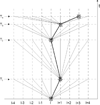
Figure 1: Paths of the LQKR wave function as a function of the angular momentum, $l$. The measurements are performed at times ${T_{i}}$ and the wave function collapses at these times. Between measurements the system has an unitary quantum evolution

The detailed mechanism to obtain the evolution is given in alejo2 . We take $\rho(T)$ in accordance with the Lévy distribution Shlesinger that includes a parameter $\alpha$, with $0<\alpha\leq 2$. When $\alpha<2$ the second moment of $\rho$ is infinite, when $\alpha=2$ the Fourier transform of $\rho$ is the Gaussian distribution and the second moment is finite. Then, this distribution has no characteristic size for the temporal jump, except in the Gaussian case. The absence of scale makes the Lévy random walks scale-invariant fractals. This means that any classical trajectory has many scales but none in particular dominates the process. This distribution appears, for example, in quantum optics Bardou as an appropriate tool to describe cooled atomic samples in terms of a competition between a trapping process (the atom falls in the optical trap) and a recycling process (the atom leaves the trap and eventually return to it). The most important characteristic of the Lévy noise is the power-law shape of the tail, accordingly in this work we use the waiting-time distribution

$$\rho(t)=\frac{\alpha}{\left(1+\alpha\right)}\left\{\begin{array}[]{cc}1,&0\leq t<1,\\ \left(\frac{1}{t}\right)^{\alpha+1},&t\geq 1.\end{array}\right.$$ (4)

To obtain the time interval $T$ we sort a continuous variable $t$ in agreement with Eq. (4) and then we take the integer part $T_{i}$ of this variable alejo2 .

In what follows we assume that the resonance condition of the QKR is satisfied, for the sake of simplicity we take $\varepsilon/\hbar=2\pi$ in such a way that the operator $U_{0}$ corresponds to the first principal resonance. This choice does not imply a loss of generality for our results as we shall show below.

Let us suppose that the wave function is measured at the time $t$, then it evolves according to the unitary map Eq. (2) during a time interval $T$, and again at this last time $t+T$ a new measurement is performed. In Fig. 1 we present a path diagram of the state evolution. It shows four time steps when the measurements are perform, between measurements there is an unitary evolution. When the measurement is performed the wave function collapses in a momentum state. The resulting states after successive measurements need not be contiguous states as in the QW because all transitions are possible.

In the figure we present a generic and arbitrary path with bold line. From this diagram we can write a dynamical equation for the probabilities of the LQKR momenta. To begin note that the probability that the wave function collapses in the eigenstate $|j\rangle$, due to a momentum measurement, starting from the eigenstate $|0\rangle$ after a time $T$ is

$$P_{j}(T)\equiv{|a_{j}({T})|\ }^{2}.$$ (5)

The momentum distribution $P_{j}$ depends on the initial state and on the time interval $T$ because of the collapse of the wave function, and it will play the role of transition probabilities for the global evolution. The mechanism used to perform momentum measurements assures that these distributions will repeat themselves around the new momentum. Then it is straightforward to build the probability distribution $P_{j}$ at the new time $t+T$ as a convolution between this distribution at the time $t$ and the conditional probability:

$$P_{l}(t+T)=\sum\limits_{j=-\infty}^{\infty}q_{l-j}(T)P_{j}(t),$$ (6)

where $q_{l-j}$ are the transition probabilities from state $j$ to state $l$ and the sum is extended between $-\infty$ and $+\infty$ because all the transition are possible. To calculate $q_{l-j}$ the original dynamical equations Eqs. (2, 3) and the properties of the Bessel function are used to obtain a connection between the initial pure state after a measurement and all possible final states before the next measurement

$$q_{l-j}(T)={(J_{j-l}(\kappa T))}^{2}.$$ (7)

The Eq. (6) is a sort of master equation, but not strictly because of the time dependence of the transition probabilities.

There are many ways of solving Eq. (6), we choose the method of the generating function $G(z.t)$ defined as

$$G(z,t)=\sum\limits_{j=-\infty}^{\infty}z^{j}P_{j}(t),$$ (8)

where we shall take the auxiliary variable $z$ as $z\equiv e^{i\varphi}$, with $\varphi$ real. It is easy to prove using Eq. (6), that

$$G(z,t+T)=G(z,t)J_{0}(2\kappa Tsin\varphi/2),$$ (9)

The first and second moments are given by

$$m_{1}(t)\equiv G^{\prime}(1,t),$$ (10)

$$m_{2}(t)\equiv G^{\prime\prime}(1,t),$$ (11)

where the prime indicates differentiation with respect to $z$. Then using these equations and Eq. (9) the following maps for the moments are obtained:

$$m_{1}(t+T) =m_{1}(t)+m_{1q}(T),$$ (12)

$$m_{2}(t+T) =m_{2}(t)+2m_{1}(t)m_{1q}(T)+m_{2q}(T),$$ (13)

where

$$m_{1q}(T) =\sum\limits_{l=-\infty}^{l=\infty}lq_{l}(T),$$ (14)

$$m_{2q}(T) =\sum\limits_{l=-\infty}^{l=\infty}l^{2}q_{l}(T).$$ (15)

Note that $m_{1q}(T)$ and $m_{2q}(T)$ are the first and second moments of the unitary evolution between measurements. From these expressions and using the Eq.(7) the following results are obtained $m_{1q}(T)=0$ and $m_{2q}(T)=\frac{1}{2}\kappa T^{2}$. Therefore the global variance $\sigma^{2}(t)=m_{2}(t)-m_{1}^{2}(t)$ verifies that

$$\sigma^{2}\left(t+T\right)=\sigma^{2}\left(t\right)+\sigma_{q}^{2}(T),$$ (16)

where $\sigma_{q}^{2}(T)=m_{2q}(T)-m_{1q}^{2}(T)=\frac{1}{2}\kappa T^{2}$ is the variance associated to the unitary evolution between measurements. Note that the value of the coefficient of $T^{2}$ is a consequence of using the principal resonance but the time dependence remains unchanged for any other resonance. From these last equations is easy to show that

$$\sigma^{2}\left(t\right)=\frac{1}{2}\kappa N\sum\limits_{i=1}^{N}T_{i}^{2},$$ (17)

where

$$t=\sum\limits_{i=1}^{N}T_{i},$$ (18)

and $N$ is the number of measurements performed. These results are generic, now we shall calculate the average of Eq. (17)

$$\left\langle\sigma^{2}\left(t\right)\right\rangle=\frac{1}{2}\kappa t\frac{\left\langle T_{i}^{2}\right\rangle}{\left\langle T_{i}\right\rangle},$$ (19)

where the relation $t={\left\langle T_{i}\right\rangle}{\left\langle N\right\rangle}$ was used. The first and the second moments of the waiting time for our Lévy distribution, Eq. (4), are

$$\left\langle T_{i}\right\rangle=\frac{\alpha}{\alpha+1}\left\{\begin{array}[]{cc}\left(\frac{1}{2}+\frac{t^{1-\alpha}-1}{1-\alpha}\right),&\alpha\neq 1,\\ \left(\frac{1}{2}+\ln(t)\right),&\alpha=1,\end{array}\right.$$ (20)

$$\left\langle T_{i}^{2}\right\rangle=\frac{\alpha}{\alpha+1}\left\{\begin{array}[]{cc}\left(\frac{1}{3}+\frac{t^{2-\alpha}-1}{2-\alpha}\right),&\alpha\neq 2,\\ \left(\frac{1}{3}+\ln(t)\right),&\alpha=2.\end{array}\right.$$ (21)

Substituting these expressions in Eq. (19) and for a large time

$$\left\langle\sigma^{2}\left(t\right)\right\rangle=\frac{1}{2}\kappa\left\{\begin{array}[]{cc}t^{2}\,,&\text{if \ }0\leqslant\alpha\leqslant 1,\\ t^{(3-\alpha)}\,,&\text{if \ }1\leqslant\alpha\leqslant 2.\end{array}\right.$$ (22)

Therefore when $t\rightarrow\infty$ the variance behaves as $\left\langle\sigma^{2}\left(t\right)\right\rangle\sim t^{2c}$ where

$$c=\left\{\begin{array}[]{cc}1\,,&\text{if \ }0\leqslant\alpha\leqslant 1,\\ \frac{1}{2}(3-\alpha)\,,&\text{if \ }1\leqslant\alpha\leqslant 2.\end{array}\right.$$ (23)

This result shows that measurements do not break completely the coherence of the system on a time scale that includes several of them. For $0\leqslant\alpha\leqslant 1$ the ballistic behavior is preserved as in the usual resonant QKR, and for $1\leqslant\alpha\leqslant 2$ it is lost and the sub-ballistic behavior takes place. When $\alpha=2$ the system has a diffusive behavior as in the usual Brownian motion. From the fact, that the exponent $c$ does not depend on $\kappa$ it follows that the results are valid for both primary and secondary resonances. However the coefficient $c$ depends on the microscopic law of evolution, $\sigma_{q}^{2}(T)\propto T^{2}$. Then, we may pose the question if there exists a relation between the time dependence of $\sigma_{q}^{2}(T)$ in the quantum unitary evolution between measurements and the exponent $c$ of the power law for the averaged variance. To answer this question we shall suppose a unitary quantum evolution that produces the following variance

$$\sigma_{q}^{2}(T)\propto T^{\beta},$$ (24)

where $\beta$ is a constant. The reasoning to obtain the exponent $c$ can now be repeated, it is only necessary to calculate again the new expression for a general $\beta$ moment with the Lévy waiting time distribution, that is

$$\left\langle T_{i}^{\beta}\right\rangle=\frac{\alpha}{\alpha+1}\left\{\begin{array}[]{cc}\left(\frac{1}{\beta+1}+\frac{t^{\beta-\alpha}-1}{\beta-\alpha}\right),&\alpha\neq\beta,\\ \left(\frac{1}{\beta+1}+\ln(t)\right).&\alpha=\beta\end{array}\right.$$ (25)

Then, in this generic case, for $t\rightarrow\infty$, the exponent $c$ is

$$c=\frac{1}{2}\left\{\begin{array}[]{cc}\beta\,,&\text{if \ }\alpha\leqslant\beta,0\leqslant\alpha\leqslant 1,\\ (\beta-\alpha+1)\,,&\text{if \ }\alpha\leqslant\beta,1\leqslant\alpha\leqslant 2,\\ \alpha\,,&\text{if \ }\beta\leqslant\alpha,0\leqslant\alpha\leqslant 1,\\ 1\,.&\text{if \ }\beta\leqslant\alpha,1\leqslant\alpha\leqslant 2\\ \end{array}\right.$$ (26)

This expression shows that these systems can exhibit diffusive, sub-diffusive, ballistic or sub-ballistic behaviors depending on the values of $\alpha$ and $\beta$. Then, in the theoretical frame of fractional dynamics sokolov Eq. (6) together with the Lévy distribution would generate a generalized master equation from which a generic fractional diffusion equation metzler could be built. This fractional dynamics approach has as an extreme case the classical diffusion equation for $\alpha=\beta=2$.

III Conclusion

The quantum resonances of the QKR have been experimentally observed in samples of cold atoms interacting with a far-detuned standing wave of laser light Moore ; Ammann . We study the QKR subjected to measurements with a Lévy waiting-time distribution. As the Gaussian distribution is a particular case of the Lévy distribution, then our study is open to wider experimental situations. We showed numerically alejo2 that a Lévy noise does not break completely the coherence in the dynamics of the QKR but produces a sub-ballistic behavior. There the system was also a LQKR but the operators $U_{0}$ and $U_{1}$ corresponded to the same secondary resonance with two different values of the strength parameter $\kappa$ and these operators do not commute. It is important to note that if the operators correspond to a primary resonance the ballistic behavior was retained due to the commutativity between the operators $U_{0}$ and $U_{1}$ alejo2 . In the present model one of the operators is unitary, and may correspond to any resonance of the QKR, and the other is the measurement operator. These operators also do not commute and again this is linked to the sub-ballistic behavior. Then we can conclude that for the LQKR the behavior of $\sigma(t)$ depends on the commutativity and the waiting time distribution, both models show the same physics. We developed a simple analytical theory to connect the waiting time parameter $\alpha$ with the exponent $c$. The LQKR behaves like the QW subjected to the same measurement process alejo3 , strengthening our previously established parallelism between both systems alejo1 ; alejo2 ; alejo4 ; alejo5 , where the resonant QKR is interpreted as a QW in momentum space. The type of model developed in this work shows that a quantum system in combination with a Lévy stochastic process leads to an anomalous diffusion and not to the well known diffusive process of Browniam motion. Finally, this simple toy model may help to understand the connection between a fractional approach and a generalized master equation.

I thank V. Micenmacher for stimulating discussions and comments. I acknowledge support from PEDECIBA and PDT S/C/IF/54/5.

References

- (1) C. Cohen-Tannoudji, Rev. Mod. Phys. 70, 707 (1998).
- (2) F. M. Izrailev, Phys. Rep. 196, 299 (1990).
- (3) J. Kempe, Contemp. Phys. 44, 302 (2003).
- (4) F.L. Moore, J.C. Robinson, C.F. Bharucha, B. Sundaram, and M.G. Raizen, Phys. Rev. Lett. 75, 4598 (1995); J.C. Robinson, C. Bharucha, F.L. Moore, R. Jahnke, G.A. Georgakis, Q. Niu, M.G. Raizen and B. Sundaram, Phys. Rev. Lett. 74, 3963 (1995); J.C. Robinson, C.F. Bharucha, K.W. Madison, F.L. Moore, Bala Sundaram, S.R. Wilkinson and M.G. Raizen, Phys. Rev. Lett. 76, 3304 (1996). F.L. Moore, J.C. Robinson, C. Bharucha, P.E. Williams and M.G. Raizen, Phys. Rev. Lett. 73, 2974 (1994).
- (5) J.F. Kanem, S. Maneshi, M. Partlow, M. Spanner and A. M. Steinberg in quant-ph/0604110.
- (6) A. Romanelli, R. Siri, and V. Micenmacher, Phys. Rev. E 76, 037202 (2007).
- (7) A. Romanelli, A. Auyuanet, R. Siri, and V. Micenmacher, Phys. Lett. A 365, 200 (2007).
- (8) P. Ribeiro, P. Milman, and R. Mosseri, Phys. Rev. Lett. 93, 190503 (2004).
- (9) A. Romanelli, Phys. Rev. A 76, 054306 (2007).
- (10) A. Romanelli, A.C. Sicardi Schifino, R. Siri, G. Abal, A. Auyuanet, and R. Donangelo. Physica A, 338, 395 (2004).
- (11) A. Romanelli, R. Siri, G. Abal, A. Auyuanet, and R. Donangelo. Physica A, 352, 409 (2005).
- (12) M.F. Shlesinger, G.M. Zaslavsky and J. Klafter, Nature (London) 363, 31 (1993); J. Klafter, M.F. Shlesinger, and G. Zumofen, Phys. Today 49 (2), 33 (1996), G.M. Zaslavsky, Phys. Today 52 (8), 39 (1999).
- (13) F. Bardou, J.P. Bouchaud, A. Aspect, C. Cohen-Tannoudji, Lévy Statistics and Laser Cooling, Cambridge University Press, Cambridge (2002).
- (14) I.M. Sokolov, J. Klafter, A. Blumen, Phys. Today, 55, 48 (2002).
- (15) R. Metzler, J. Klafter, Phys. Rep., 339, 1 (2000).
- (16) H. Ammann, R. Gray, I. Shvarchuck and N. Christensen, Phys. Rev. Lett. 80, 4111 (1998).