Free expansion of a Lieb-Liniger gas: Asymptotic form of the wave functions

Abstract

The asymptotic form of the wave functions describing a freely expanding Lieb-Liniger gas is derived by using a Fermi-Bose transformation for time-dependent states, and the stationary phase approximation. We find that asymptotically the wave functions approach the Tonks-Girardeau (TG) structure as they vanish when any two of the particle coordinates coincide. We point out that the properties of these asymptotic states can significantly differ from the properties of a TG gas in a ground state of an external potential. The dependence of the asymptotic wave function on the initial state is discussed. The analysis encompasses a large class of initial conditions, including the ground states of a Lieb-Liniger gas in physically realistic external potentials. It is also demonstrated that the interaction energy asymptotically decays as a universal power law with time, $E_{\mathrm{int}}\propto t^{-3}$.

HD–THEP–08–10

I Introduction

The physics of one-dimensional (1D) Bose gases in many aspects differs from the physics encountered in higher dimensional systems. For example, the Lieb-Liniger (LL) gas of $\delta$-interacting bosons in one spatial dimension becomes less ideal as its density decreases Lieb1963 , and eventually approaches the Tonks-Girardeau (TG) limit of a gas of ”impenetrable-core” bosons Girardeau1960 as it becomes sufficiently diluted. The interest in these 1D systems is greatly stimulated by their experimental realization with atoms confined in tight 1D atomic wave guides OneD ; TG2004 ; Kinoshita2006 . The special features of effectively 1D atomic gases Olshanii ; Petrov ; Dunjko are reflected by properties of nonequilibrium dynamics in these systems, which have become accessible experimentally Kinoshita2006 . The possibility of finding exact time-dependent solutions for LL Gaudin1983 ; Girardeau2003 ; Buljan2008 and TG Girardeau2000 ; Girardeau2000a ; Ohberg2002 ; Busch2003 ; Rigol2005 ; Minguzzi2005 ; DelCampo2006 ; Rigol2006 ; Buljan2006 ; Pezer2007 ; Gangardt2007 evolution is of particular theoretical interest, as they have the potential to provide insight beyond various approximation schemes.

Exact solutions for a homogeneous Bose gas with (repulsive) point-like interactions of arbitrary strength $c$, and periodic boundary conditions, were presented by Lieb and Liniger in 1963 Lieb1963 . For attractive interactions, $c<0$, exact LL wave functions were analyzed in Ref. McGuire1964 . The case of box confinement for $c>0$ was studied in Ref. Gaudin1971 . In the light of recent experiments OneD ; TG2004 ; Kinoshita2006 exact studies of the LL model are even more attractive today Muga1998 ; Sakmann2005 ; Batchelor2005 ; Kinezi2006 ; Sykes2007 . Besides providing insight into the physics of 1D Bose gases, exact solutions can serve as a benchmark for various approximations as well as for numerical approaches (see, e.g., Refs. Sykes2007 ; Kanamoto2005 ). The calculation of correlation functions of a LL gas from the wave functions is a difficult task; these functions furnish observables like the momentum distribution of particles in the gas, and were studied by using various approaches (e.g., see Refs. Creamer1981 ; Jimbo1981 ; Korepin1993 ; Kojima1997 ; Olshanii2003 ; Gangardt2003 ; Astrakharchik2003 ; Kheruntsyan2005 ; Forrester2006 ; Caux2007 ; Calabrese2007 ; Khodas2007 ). Time-dependent phenomena in the context of LL gases with finite-strength interactions have been addressed by using both analytical Gaudin1983 ; Girardeau2003 ; Buljan2008 and numerical methods (see, e.g., Refs. Berman2004 ; Li2005 ). Irregular dynamics of a LL gas was studied numerically in a mesoscopic system in Ref. Berman2004 . In Ref. Girardeau2003 , it was shown that phase imprinting by light pulses conserves the so-called cusp condition for the LL wave function imposed by the interactions.

Exact solutions for 1D Bose gases are conveniently constructed by using the Fermi-Bose mapping techniques Girardeau1960 ; Gaudin1983 ; Girardeau2000 ; Das2002 . In 1960 Girardeau discovered that the wave function of a spinless noninteracting 1D Fermi gas can be symmetrized such that it describes an impenetrable-core 1D Bose gas Girardeau1960 . This mapping is valid for arbitrary external potentials Girardeau1960 , for time-dependent problems Girardeau2000 , and in the context of statistical mechanics Das2002 . In fact, fermion-boson duality in 1D exists for arbitrary interaction strengths Cheon1999 ; Yukalov2005 . Furthermore, a time-dependent antisymmetric wave function describing a 1D system of noninteracting fermions can be transformed, by using a differential Fermi-Bose mapping operator, to an exact time-dependent solution for a LL gas, as outlined by Gaudin Gaudin1983 . This method is applicable in the absence of external potentials and other boundary conditions. Therefore, it is particularly useful to study free expansion of LL gases from an initially localized state.

Free expansion of interacting Bose gases has recently attracted considerable attention. It has been utilized in experiments to deduce information on the initial state (see, e.g., Ref. Bloch2008 and references therein), and can be considered as a quantum-quench-type problem which provides insight into the relaxation of quantum systems (see, e.g., Refs. Calabrese2007a ; Rigol2007a and references therein). Free expansion of a LL gas has been analyzed in Ref. Ohberg2002 by employing the hydrodynamic formalism Dunjko ; it was shown that the density of the gas does not follow self-similar evolution Ohberg2002 . However, in 1D Bose systems, most exact many-body solutions are given for the TG gas Ohberg2002 ; Rigol2005 ; Minguzzi2005 ; DelCampo2006 ; Gangardt2007 . An important result is that the momentum distribution of the freely expanding TG gas asymptotically approaches the momentum distribution of free fermions Rigol2005 ; Minguzzi2005 . Recently, we have constructed a particular family of exact solutions describing a LL gas freely expanding from a localized initial density distribution Buljan2008 . It was shown that for any interaction strength, the wave functions asymptotically (as $t\rightarrow\infty$) assume TG form. Even though it is generally accepted that 1D Bose gases become less ideal with decreasing density, this intuition is mainly based on the studies of a LL gas in equilibrium ground states Lieb1963 . Thus, a more rigorous analysis of the expanding LL gas, which leads to more dilute system, but out of equilibrium, is desirable. In particular, it is interesting to study the dependence of the asymptotic wave functions on the initial state, and to see how are the initial conditions imprinted in the asymptotic states.

Here we study the asymptotic form of the wave function describing a freely expanding Lieb-Liniger gas, which can be constructed via the Fermi-Bose transformation and the stationary phase approximation. In Section II we describe the LL model and the Fermi-Bose transformation. In Section III we demonstrate that the asymptotic wave functions have Tonks-Girardeau structure, that is, they vanish when any of the two particle coordinates coincide. The dependence of the asymptotic state on the initial state is discussed. We illustrate that the properties of the asymptotic wave functions can significantly differ from the properties of a TG gas in the ground state of some external potential. This study generalizes and adds upon our previous result from Ref. Buljan2008 , as the initial conditions studied here encompass ground states for generic external potentials and various interaction strengths. From the next-to-leading order term in the asymptotic regime, we deduce that the interaction energy of the LL gas decays as a universal power law in time $E_{\mathrm{int}}\propto t^{-3}$. This is illustrated on a particular example in Section IV, where we provide further analysis of the particular family of time-dependent LL wave functions studied in Ref. Buljan2008 . Explicit expressions for the asymptotic form of the single-particle density are provided in Section V. In Section VI we calculate the asymptotic single-particle density for free expansion of a LL gas from an infinitely deep box potential. We compare our exact calculation with the hydrodynamic approximation introduced in Ref. Dunjko , and employed in Ref. Ohberg2002 in the context of free expansion, obtaining good agreement for all values of the interaction strength.

II The Lieb-Liniger model

A system of $N$ identical $\delta$-interacting bosons in one spatial dimension is described by the many-body Schrödinger equation Lieb1963

$$i\frac{\partial\psi_{B}}{\partial t}=-\sum_{i=1}^{N}\frac{\partial^{2}\psi_{B}}{\partial x_{i}^{2}}+\sum_{1\leq i<j\leq N}2c\,\delta(x_{i}-x_{j})\psi_{B}.$$ (1)

Here, $\psi_{B}(x_{1},\ldots,x_{N},t)$ is the time-dependent wave function, and $c$ is the strength of the interaction. It is assumed that the initial wave function is localized, e.g., by the system being trapped within some external potential, before, at $t=0$, the trap is suddenly switched off and the gas starts expanding. We are interested in the behavior of $\psi_{B}$ when $t\rightarrow\infty$. Here the spatial dimension is infinite $x_{j}\in(-\infty,\infty)$, i.e., we do not impose any boundary conditions.

Due to the Bose symmetry of the wave function, it is sufficient to express it in the fundamental sector of the configuration space, $R_{1}:x_{1}<x_{2}<\ldots<x_{N}$, where $\psi_{B}$ obeys

$$i\frac{\partial\psi_{B}}{\partial t}=-\sum_{i=1}^{N}\frac{\partial^{2}\psi_{B}}{\partial x_{i}^{2}}.$$ (2)

The $\delta$-interactions create a cusp in the wave function when two particles touch. This can be expressed as a boundary condition at the borders of $R_{1}$ Lieb1963 :

$$\left[1-\frac{1}{c}\left(\frac{\partial}{\partial x_{j+1}}-\frac{\partial}{\partial x_{j}}\right)\right]_{x_{j+1}=x_{j}}\psi_{B}=0.$$ (3)

These boundary conditions can easily be rewritten for any permutation sector. In the TG limit, i.e., for $c\rightarrow\infty$, the cusp condition implies that the wave function vanishes when two particles are in contact: $\psi_{B}(x_{1},\ldots,x_{j},x_{j+1},\ldots,x_{N},t)|_{x_{j+1}=x_{j}}=0$ Girardeau1960 ; Girardeau2000 .

Exact solutions of the time-dependent Schrödinger equation (1) can be obtained by using a Fermi-Bose mapping operator Gaudin1983 ; Buljan2008 acting on fermionic wave functions: If $\psi_{F}(x_{1},\ldots,x_{N},t)$ is an antisymmetric (fermionic) wave function, which obeys the Schrödinger equation for a noninteracting Fermi gas,

$$i\frac{\partial\psi_{F}}{\partial t}=-\sum_{i=1}^{N}\frac{\partial^{2}\psi_{F}}{\partial x_{i}^{2}},$$ (4)

then the wave function

$$\psi_{B,c}={\mathcal{N}}_{c}\hat{O}_{c}\psi_{F},$$ (5)

where

$$\hat{O}_{c}=\prod_{1\leq i<j\leq N}\left[\mbox{sgn}(x_{j}-x_{i})+\frac{1}{c}\left(\frac{\partial}{\partial x_{j}}-\frac{\partial}{\partial x_{i}}\right)\right],$$ (6)

is the differential Fermi-Bose mapping operator, and ${\mathcal{N}}_{c}$ is a normalization constant, obeys Eq. (1) Gaudin1983 . For the purpose of completeness we outline, in Appendix A, the proof that the wave function (5) obeys both the cusp condition imposed by the interactions and the Schrödinger equation (2).

III Free expansion: Asymptotics

In this section we study the asymptotic form of time-dependent LL wave functions $\psi_{B,c}$ which are obtained by the Fermi-Bose transformation (5). All information on the initial condition $\psi_{B,c}(x_{1},\ldots,x_{N},t=0)$ is contained in the initial fermionic wave function $\psi_{F}(x_{1},\ldots,x_{N},t=0)$:

$$\psi_{B,c}(x_{1},\ldots,x_{N},0)={\mathcal{N}}_{c}\hat{O}_{c}\psi_{F}(x_{1},\ldots,x_{N},0).$$ (7)

The initial bosonic wave function, which can be expressed in this way, is assumed to describe a LL gas in its ground state when trapped in some external potential $V(x)$, e.g., in a harmonic oscillator potential, or some other trapping potential used in experiments. We consider the evolution from this initial state after the trapping potential has been suddenly turned off, as studied in experiments to deduce information on the initial state Bloch2008 . The time-dependent fermionic wave function $\psi_{F}(x_{1},\ldots,x_{N},t)$, which freely expands from the initial condition $\psi_{F}(x_{1},\ldots,x_{N},0)$, can be expressed in terms of its Fourier transform,

$$\psi_{F}(x_{1},\ldots,x_{N},t)=\int dk_{1}\cdots dk_{N}$$

$$\quad\times\ \tilde{\psi}_{F}(k_{1},\ldots,k_{N})e^{i\sum_{j=1}^{N}[k_{j}x_{j}-\omega(k_{j})t]},$$ (8)

where $\omega(k)=k^{2}$, and

$$\tilde{\psi}_{F}(k_{1},\ldots,k_{N})=\frac{1}{(2\pi)^{N}}\int dx_{1}\cdots dx_{N}$$

$$\quad\times\ \psi_{F}(x_{1},\ldots,x_{N},t=0)e^{-i\sum_{j=1}^{N}k_{j}x_{j}}.$$ (9)

By using the Fermi-Bose transformation, the time-dependent bosonic wave function describing the freely expanding LL gas can be expressed as

$$\psi_{B,c}=\int dk_{1}\cdots dk_{N}$$

$$\quad\times\ G(k_{1},\ldots,k_{N})e^{i\sum_{j=1}^{N}[k_{j}x_{j}-\omega(k_{j})t]},$$ (10)

where the function $G(k_{1},\ldots,k_{N})$ is defined as

$$G(k_{1},\ldots,k_{N})={\mathcal{N}}_{c}\tilde{\psi}_{F}(k_{1},\ldots,k_{N})$$

$$\quad\times\ \prod_{1\leq i<j\leq N}[\mbox{sgn}(x_{j}-x_{i})+\frac{i}{c}(k_{j}-k_{i})].$$ (11)

It should be noted that $G(k_{1},\ldots,k_{N})$ is not the Fourier transform of $\psi_{B,c}$ because it depends on $x_{j}$ through the $\mbox{sgn}(x_{j}-x_{i})$ terms.

The asymptotic form of the wave function (10) can be obtained by evaluating the integral with the stationary phase approximation. The phase $\phi=\sum_{j=1}^{N}[k_{j}x_{j}-\omega(k_{j})t]$ is stationary when $\partial\phi/\partial k_{j}=0$. Let $\{k^{{}^{\prime}}_{j}\}$ denote the $k_{j}$-values for which

$$\left.\frac{\partial\phi}{\partial k_{j}}\right|_{k^{{}^{\prime}}_{j}}=x_{j}-2k^{{}^{\prime}}_{j}t=0,$$

that is, $k^{{}^{\prime}}_{j}=x_{j}/2t$. The phase can be rewritten as

$$\phi(\{k\})=\phi(\{k^{{}^{\prime}}\})-t\sum_{j=1}^{N}(k_{j}-k^{{}^{\prime}}_{j})^{2}.$$

The leading term of the integral in Eq. (10), as well as the next-to-leading term, can be evaluated by expanding $G(k_{1},\ldots,k_{N})\equiv G(\{k\})$ in a Taylor series around the stationary phase point $\{k^{{}^{\prime}}\}$:

$$\psi_{B,c}\ =\ e^{i\phi(\{k^{{}^{\prime}}\})}\Big{[}G(\{k^{{}^{\prime}}\})\int dk_{1}\cdots dk_{N}e^{-it\sum_{j=1}^{N}(k_{j}-k^{{}^{\prime}}_{j})^{2}}$$

$$+\ \sum_{i=1}^{N}\left.\frac{\partial G(\{k\})}{\partial k_{i}}\right|_{\{k^{{}^{\prime}}\}}\int dk_{1}\cdots dk_{N}(k_{i}-k^{{}^{\prime}}_{i})e^{-it\sum_{j=1}^{N}(k_{j}-k^{{}^{\prime}}_{j})^{2}}$$

$$+\ \frac{1}{2!}\sum_{i,j=1}^{N}\left.\frac{\partial^{2}G(\{k\})}{\partial k_{i}\partial k_{j}}\right|_{\{k^{{}^{\prime}}\}}\int dk_{1}\cdots dk_{N}(k_{i}-k^{{}^{\prime}}_{i})(k_{j}-k^{{}^{\prime}}_{j})e^{-it\sum_{l=1}^{N}(k_{l}-k^{{}^{\prime}}_{l})^{2}}\ +\ldots\Big{]}.$$ (12)

The remaining integrals in the three terms written out in this expansion can be calculated analytically. The second term involving the first derivatives of $G(\{k\})$ vanishes. The third term is nonvanishing only for $i=j$. Thus Eq. (12) reduces to

$$\psi_{B,c} =e^{i\phi(\{k^{{}^{\prime}}\})}\left(\sqrt{\frac{\pi}{t}}e^{-i\pi/4}\right)^{N}$$

$$\qquad\Big{[}G(\{k^{{}^{\prime}}\})-\frac{i}{4t}\sum_{i=1}^{N}\left.\frac{\partial^{2}G(\{k\})}{\partial k^{2}_{i}}\right|_{\{k^{{}^{\prime}}\}}+\ldots\Big{]}.$$ (13)

From Eq. (13) we obtain in leading order the asymptotic wave function

$$\psi_{\infty} \propto\ t^{-{N}/{2}}\prod_{1\leq i<j\leq N}\Big{[}\mathrm{sgn}(x_{j}-x_{i})+\frac{i}{c}(k^{{}^{\prime}}_{j}-k^{{}^{\prime}}_{i})\Big{]}$$

$$\quad\times\ \tilde{\psi}_{F}(k^{{}^{\prime}}_{1},\ldots,k^{{}^{\prime}}_{N})e^{i\sum_{j=1}^{N}[k^{{}^{\prime}}_{j}x_{j}-\omega(k^{{}^{\prime}}_{j})t]},$$ (14)

which is written in a more convenient form in terms of the variables $\xi_{j}=x_{j}/t$:

$$\psi_{\infty} \propto\ t^{-{N}/{2}}\prod_{1\leq i<j\leq N}\Big{[}\mathrm{sgn}(\xi_{j}-\xi_{i})+\frac{i}{2c}(\xi_{j}-\xi_{i})\Big{]}$$

$$\quad\times\ \tilde{\psi}_{F}(\xi_{1}/2,\ldots,\xi_{N}/2)\,e^{\frac{i}{4}\sum_{j=1}^{N}\xi_{j}^{2}t}.$$ (15)

Equation (15) is the main result of this paper. Evidently the asymptotic form of the LL wave function $\psi_{\infty}$ has TG form. Namely, the Fourier transform of a fermionic wave function $\tilde{\psi}_{F}(\xi_{1}/2,\ldots,\xi_{N}/2)$ is antisymmetric, which implies that $\psi_{\infty}$ is zero whenever $\xi_{i}=\xi_{j}$ $(i\neq j)$. Furthermore, $\psi_{\infty}$ is symmetric under the exchange of any two coordinates $\xi_{i}$ and $\xi_{j}$. This clearly shows that a localized LL wave function during free expansion asymptotically approaches a wave function with the TG structure. However, it should be emphasized that the properties of the asymptotic state are not necessarily similar to the wave function describing TG gas in equilibrium, in the ground state of some external potential. The connection between the initial and the asymptotic state is illustrated below.

In the derivation of Eq. (15) we have analyzed LL wave functions which are obtained through the Fermi-Bose transformation (5). This class of wave functions is quite general and corresponds to numerous situations of practical relevance. Let us discuss the case in which the initial bosonic wave function $\psi_{B0}=\psi_{B,c}(x_{1},\ldots,x_{N},0)$ is a ground state of a repulsive LL gas in an experimentally realistic external potential $V(x)$, e.g., a harmonic oscillator potential. The eigenstates of the LL system in free space are of the form

$$\psi_{\{k\}}=\mathcal{N}({\{k\}})\hat{O}_{c}\det[e^{ik_{m}x_{j}}]_{m,j=1}^{N},$$ (16)

where the set of $N$ real values $\{k\}=\{k_{m}\,|\,m=1,\ldots,N\}$ uniquely determines the eigenstate; the normalization constant is given by

$$\frac{1}{\mathcal{N}({\{k\}})}=\sqrt{(2\pi)^{N}N!\prod_{i<j}{\left[1+\left(\frac{k_{j}-k_{i}}{c}\right)^{2}\right]}},$$

see Ref. Korepin1993 . In free space, there are no restrictions on the numbers $k_{m}$. If periodic boundary conditions are imposed as in Ref. Lieb1963 (i.e., the system is a ring of length $L$), the wave numbers $k_{j}$ must obey a set of coupled transcendental equations Lieb1963 ; Muga1998 ; Sakmann2005 ; Forrester2006 ; Sykes2007 which depend on the strength of the interaction (see, e.g., Ref. Sakmann2005 ). The LL eigenstates $\psi_{\{k\}}$ possess the closure property Gaudin1983 and they are complete Dorlas1993 . Thus, our initial state $\psi_{B0}$ can be expressed as a superposition of LL eigenstates,

$$\psi_{B0} = \sum_{\{k\}}b(\{k\})\psi_{\{k\}}$$ (17)

$$= \hat{O}_{c}\sum_{\{k\}}\mathcal{N}({\{k\}})b(\{k\})\det[e^{ik_{m}x_{j}}]_{m,j=1}^{N},$$

where the coefficients $b(\{k\})$ can be obtained by projecting the initial condition $\psi_{B0}$ onto the LL eigenstates. By comparing Eqs. (7) and (17) we find that the initial fermionic wave function is

$$\psi_{F0}={\mathcal{N}}_{c}^{-1}\sum_{\{k\}}\mathcal{N}({\{k\}})b(\{k\})\det[e^{ik_{m}x_{j}}]_{m,j=1}^{N}.$$ (18)

Since we have assumed that $V(x)$ is an experimentally realistic smooth function, also $\psi_{F0}$ is smooth and differentiable such that the operator $\hat{O}_{c}$ can be applied.

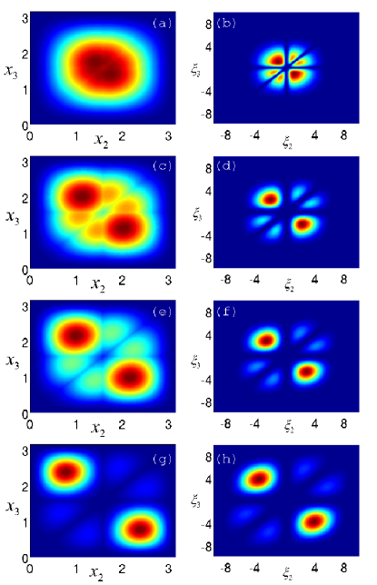
Figure 1: (color online) Contour plots illustrating free expansion of $N=3$ bosons from the ground state of a LL gas in a box with infinitely high walls ($L=\pi$). The left column depicts the initial ground state $|\psi_{B0}(L/2,x_{2},x_{3})|^{2}$, and the right column depicts the asymptotic state $|\psi_{\infty}(0,\xi_{2},\xi_{3})|^{2}$, for $c=0.2$ (a,b), $c=1$ (c,d), $c=2$ (e,f), and $c=10$ (g,h). The density of the asymptotic state is zero when two coordinates $\xi_{i}$ and $\xi_{j}$ ($i\neq j$) coincide.

The connection between the asymptotic state (15) and the initial state $\psi_{B0}$ is made through the Fourier transform of the initial fermionic wave function $\tilde{\psi}_{F}(\{k\})$. More insight into the connection between the initial state and the asymptotic state can be made by expressing $\tilde{\psi}_{F}(\{k\})$ through the coefficients $b(\{k\})$ utilized in the expansion (17). First, let us note that the coefficients $b(\{k\})=b(k_{1},k_{2},\ldots,k_{N})$ are antisymmetric with respect to the interchange of any two arguments $k_{i}$ and $k_{j}$ $(i\neq j)$. This follows from the fact that the LL eigenstates $\psi_{\{k\}}$ possess the same property, see Ref. Korepin1993 . By using this property of $b(\{k\})$, Eq. (18) can be rewritten as

$$\psi_{F0} ={\mathcal{N}}_{c}^{-1}\sum_{\{k\}}\mathcal{N}({\{k\}})b(\{k\})\sum_{P}(-)^{P}e^{i\sum_{j=1}^{N}k_{Pj}x_{j}}$$

$$={\mathcal{N}}_{c}^{-1}\sum_{P}\sum_{\{k\}}\mathcal{N}(k_{P1},k_{P2},\ldots,k_{PN})$$

$$\times b(k_{P1},k_{P2},\ldots,k_{PN})e^{i\sum_{j=1}^{N}k_{Pj}x_{j}}$$

$$={\mathcal{N}}_{c}^{-1}N!\sum_{\{k\}}\mathcal{N}(\{k\})b(\{k\})e^{i\sum_{j=1}^{N}k_{j}x_{j}}.$$ (19)

By comparing Eqs. (19) and (8) we obtain

$$\tilde{\psi}_{F}(\{k\}) ={\mathcal{N}}_{c}^{-1}N!\mathcal{N}(\{k\})b(\{k\}).$$ (20)

Evidently, the Fourier transform of the initial fermionic wave function $\tilde{\psi}_{F}(\{k\})$ is directly proportional to the projections $b(\{k\})$ of the initial bosonic wave function onto the LL eigenstates. From this relation we can conclude that the asymptotic wave function (15) has TG structure as a consequence of the antisymmetry of the coefficients $b(\{k\})$, which originates from the antisymmetry of the LL eigenstates with respect to $k_{j}$ arguments Korepin1993 . It is also worthy to note that Eq. (10), and therefore our main result, can be obtained without explicit use of the Fermi-Bose transformation; by writing the time dependent LL states as $\psi_{B,c}=\sum_{\{k\}}b(\{k\})\psi_{\{k\}}\exp(-i\sum_{j}k_{j}^{2}t)$, and after employing the antisymmetry of $b(\{k\})$ [equivalently as in Eq. (19)] one obtains Eq. (10). Formulae (15) and (20) provide, under general conditions, the asymptotic form of the wave functions for the freely expanding LL gas, and the connection between these asymptotic states and the initial states.

For the sake of the clarity of the paper, let us illustrate the asymptotic state of the LL gas on a particular example. Suppose that initially the LL gas is in the ground state, enclosed in an infinitely deep box of length $L$. The ground state $\psi_{B0}$ for this potential was found by employing the superposition of the Bethe ansatz wave functions in Ref. Gaudin1971 . The coefficients $b(\{k\})$ can be relatively easily found for a few particles by employing a computer program for algebraic manipulation (Mathematica). In Fig. 1 we illustrate the initial state and the asymptotic state for the case of $N=3$ particles, and for values of $c=0.2,1,2$, and $10$, by showing the contour plots of the probabilities $|\psi_{B0}(L/2,x_{2},x_{3})|^{2}$ (left column) and $|\psi_{\infty}(0,\xi_{2},\xi_{3})|^{2}$ (right column). Thus, one particle is fixed in the center of the system, while the plots illustrate the probability of finding the other two particles in space. The left column illustrating the initial states shows that the system becomes more correlated with increasing interaction strenght $c$ and it enters the TG regime for sufficiently large $c$ (e.g., for $c=10$ depicted in Fig. 1 (g) the ground state of the system is in the TG regime). The right column illustrating the asymptotic state shows that the wave function is zero whenever two of the coordinates coincide. However, it is important to note that the properties of the asymptotic wave functions, even though they possess the TG structure, can significantly differ from the properties of the TG gas in the equilibrium ground state. This can be seen by comparing the asymptotic state in Fig. 1 (b), and the TG ground state shown in Fig. 1 (g). The asymptotics of Fig. 1 (b) is obtained after free expansion from a weakly interacting ground state $(c=0.2)$; from Fig. 1 (b) we observe that when one particle is fixed at zero, there is still a relatively large probability of finding the other two particles to the left and to the right of the fixed one. In contrast, for the TG ground state shown in Fig. 1 (g), if one particle is fixed in the center of the system, the other two are on the opposite sides of that one. Furthermore, by comparing the asymptotic states in Figs. 1 (b), (d), (f), and (h), we see that their properties depend on the interaction strength $c$. It is worthy to mention again that free expansion can be utilized to deduce information on the initial state (see, e.g., Refs. Bloch2008 and references therein); free 1D expansion can distinguish between different initial regimes of the LL gas Ohberg2002 .

Let us now address the case of attractive interactions. For $c<0$, the cusp condition assumes a form that is identical to that for $c>0$ (see, e.g., Ref. Muga1998 ). Therefore, by acting on some fermionic time-dependent wave function obeying Eq. (4) with the Fermi-Bose transformation operator $\hat{O}_{c<0}$, one obtains an exact solution for the attractive time-dependent LL gas in the form $\hat{O}_{c<0}\psi_{F}$ (see Appendix A); our derivation holds for this family of wave functions. Experiments where the attractive quasi-1D Bose gas is suddenly released from a trapping potential were used to study solitons made of attractively interacting BEC Khaykovich2002 . Exact studies of such a system within the framework of the LL model are expected to provide deeper insight into nonequilibrium phenomena beyond the Gross-Pitaevskii mean-field regime, where interesting dynamical effects can occur Streltsov2008 ; Buljan2005 .

It should be noted that the time scale it takes for the LL system to reach the TG regime depends on the initial condition. The next-to-leading term of the asymptotic wave function is suppressed relative to the leading term by a factor $1/t$, as obtained by the stationary phase expansion in Eq. (13). From this we can deduce the scaling of the interaction energy, defined as

$$E_{\mathrm{int}} =2c\int dx_{1}\cdots dx_{N}\,|\psi_{B,c}|^{2}\sum_{1\leq i<j\leq N}\delta(x_{i}-x_{j}),$$ (21)

as $t\rightarrow\infty$. Since the interaction strength $c$ is finite, and since the asymptotic density $|\psi_{\infty}(\xi_{1},\ldots,\xi_{N},t)|^{2}$ equals zero for any pair of arguments being equal, $\xi_{i}=\xi_{j}$, one concludes that asymptotically the leading term of the interaction energy vanishes. Since the first correction to the leading TG term of the wave function is of order $t^{-1}$, and since $\delta(x_{i}-x_{j})=t^{-1}\delta(\xi_{i}-\xi_{j})$, the interaction energy asymptotically decays to zero as $E_{\mathrm{int}}\propto t^{-3}$. This power law decay of the interaction energy is illustrated in the following section.

IV Example: Fermionic wave function expanding from a harmonic trap

In Ref. Buljan2008 , we have constructed a particular family of time-dependent wave functions describing a freely expanding LL gas. The wave functions were obtained by acting with the Fermi-Bose mapping operator onto a specific time-dependent fermionic wave function,

$$\psi_{F} \propto \exp\Big{\{}-i\frac{N^{2}\nu}{2}\tau(t)-\frac{\nu-i\nu^{2}t}{4}\sum_{j=1}^{N}\Big{[}\frac{x_{j}}{b(t)}\Big{]}^{2}\Big{\}}$$ (22)

$$\times\ b(t)^{-{N^{2}}/{2}}\prod_{1\leq i<j\leq N}(x_{j}-x_{i}),$$

which describes free expansion of noninteracting fermions in one spatial dimension. The initial fermionic wave function at $t=0$ corresponds to a fermionic ground state in a harmonic trap $V(x)=\nu^{2}x^{2}/4$ (see, e.g., Ref. Girardeau2001 ). Here, $\nu$ corresponds to the trapping frequency, $b(t)=\sqrt{1+t^{2}\nu^{2}}$, and $\tau(t)=\arctan(\nu t)/\nu$. The limiting form of the LL wave function, $\psi_{B,c}(\eta_{1}b(t),\ldots,\eta_{N}b(t),t)$, for $t\rightarrow\infty$, was shown to have the following form characteristic for a TG gas:

$$\psi_{B,c}(\eta_{1}b(t),\ldots,\eta_{N}b(t),t)\propto b(t)^{-{N}/{2}}$$

$$\quad\times\ \exp\Big{\{}-i\frac{N^{2}\nu}{2}\tau(t)-\frac{\nu-i\nu^{2}t}{4}\sum_{j=1}^{N}\eta_{j}^{2}\Big{\}}$$

$$\quad\times\ \prod_{1\leq i<j\leq N}g(\eta_{j}-\eta_{i})+{\mathcal{O}}({1}/{t}),$$ (23)

where $g(\eta)=|\eta|+i\nu\eta^{2}/2c$. Equation (15) is a generalization of this result given first in Ref. Buljan2008 .

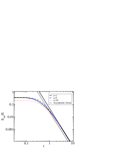
Figure 2: (color online) Time-evolution of the interaction energy $E_{\mathrm{int}}(t)$, expressed in units of the total energy $E$. The three curves correspond to values of $c=1$ (solid line), $c=5$ (dashed line), and $c=10$ (dotted line). The straight lines depict the asymptotic power law behavior of the interaction energy, $E_{\mathrm{int}}(t)\propto t^{-3}$ (see text for details).

Since Eq. (15) was obtained with the help of the stationary phase approximation, whereas (23) is obtained straightforwardly from the exact form of the specific LL wave function (see Ref. Buljan2008 ), it is worthy to verify that Eq. (15) reproduces Eq. (23) as a special case. In order to do so, we calculate the Fourier transform of the initial fermionic wave function, i.e., $\psi_{F}(x_{1},\ldots,x_{N},0)$ from Eq. (22). Interestingly, the Fourier transform has exactly the same functional form as the initial condition in $x$-space:

$$\tilde{\psi}_{F}\propto e^{-\sum_{j=1}^{N}k_{j}^{2}/\nu}\prod_{1\leq i<j\leq N}(k_{j}-k_{i}).$$ (24)

By plugging this form into Eq. (15) we obtain:

$$\psi_{\infty} \propto t^{-{N}/{2}}e^{-\sum_{j=1}^{N}\xi_{j}^{2}/(4\nu)}e^{({i}/{4})\sum_{j=1}^{N}\xi_{j}^{2}t}$$ (25)

$$\times\ \prod_{1\leq i<j\leq N}[|\xi_{j}-\xi_{i}|+\frac{i}{2c}(\xi_{j}-\xi_{i})^{2}].$$

After replacing $\xi_{j}=x_{j}/t$ with $\nu\eta_{j}=\nu x_{j}/b(t)$ which asymptotically approaches $\nu\eta_{j}\sim x_{j}/t=\xi_{j}$, we obtain the functional form identical to Eq. (23). This verifies the validity of Eq. (15) in the special case studied in Ref. Buljan2008 .

In order to verify the asymptotic power law decay of the interaction energy $E_{\mathrm{int}}$ obtained in the previous section, let us calculate the time-evolution of $E_{\mathrm{int}}$ for the specific family of LL wave functions discussed in this section. We calculate integral (21) for $N=3$ particles, and $\nu=2$. Given these parameters, $E_{\mathrm{int}}$ depends on the strength of the interaction $c$ and time $t$. Figure 2 illustrates time-evolution of the interaction energy for three values of $c$; displayed curves depict the ratio $E_{\mathrm{int}}(t)/E$, where $E$ denotes the total energy, which is a constant of motion. Evidently, after some initial transient period the interaction energy starts its asymptotic power law decay $E_{\mathrm{int}}(t)\propto t^{-3}$. It should be noted that the contribution of the interaction energy to the total energy depends on the interaction strength $c$. This is illustrated in Fig. 3 which shows $E_{\mathrm{int}}(t)/E$ as a function of $c$ at three points in time. At $t=0$, the contribution of the interaction energy to the total energy is non-monotonous with the increase of $c$; it is zero at $c=0$ and in the TG limit $c\rightarrow\infty$, with a specific maximal value in between. The form of the curve is preserved for finite values of $t$, with the evident decay of the interaction energy to zero as $t\rightarrow\infty$. Note that an equivalent non-monotonous behavior of the interaction energy as a function of $c$ was found for the Lieb-Liniger gas in the ground state for $c>0$ and with periodic boundary conditions Muga1998 .

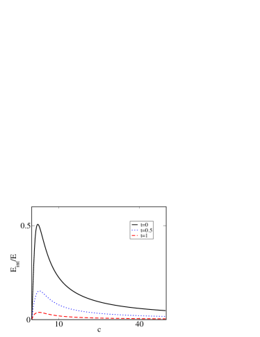
Figure 3: (color online) The ratio $E_{\mathrm{int}}/E$ as a function of the interaction strength $c$, at three values of time, $t=0$ (solid line), $t=0.5$ (dotted line), and $t=1$ (dashed line) (see text for details).

V Asymptotic single-particle density

Given the asymptotic form of the wave function, we finally consider the asymptotic form of the single-particle density which is of considerable interest for experiment. The single-particle density is defined as $\rho_{c}(x,t)=N\int dx_{2}\cdots dx_{N}|\psi_{B,c}(x,x_{2},\ldots,x_{N},t)|^{2}$. For studying asymptotics, it is convenient to define the asymptotic form in terms of the rescaled coordinates $\xi=x/t$:

$$\rho_{\infty}(\xi)={\cal N}_{\infty}t^{N}\int_{-\infty}^{\infty}d\xi_{2}\ldots d\xi_{N}|\psi_{\infty}(\xi,\xi_{2},\ldots,\xi_{N},t)|^{2};$$ (26)

here the normalization constant ${\cal N}_{\infty}$ is chosen such that $\int d\xi\,\rho_{\infty}(\xi)=N$, the total number of particles, while the factor $t^{N}$ cancels the trivial time-scaling of the asymptotic single-particle density.

For the specific asymptotic form of the wave function (25) we can analytically calculate the asymptotic form of the density for a few particles. As an example, for $N=3$, the normalization constant is

$${\cal N}_{\infty,N=3}=\frac{c^{6}}{\sqrt{2\pi^{3}\nu^{9}}(8c^{6}+48c^{4}\nu+90c^{2}\nu^{2}+45\nu^{3})},$$ (27)

while the single-particle density has the following structure:

$$\rho_{\infty}(\xi) = {\cal N}_{\infty,N=3}\frac{\pi\nu^{2}}{8c^{6}}e^{-{\xi^{2}}/(2\nu)}$$

$$\times\ [32c^{6}(3\nu^{2}+\xi^{4})$$

$$+\ 16c^{4}(33\nu^{3}-3\nu^{2}\xi^{2}+9\nu\xi^{4}+\xi^{6})$$

$$+\ 2c^{2}(465\nu^{4}-60\nu^{3}\xi^{2}+90\nu^{2}\xi^{4}+20\nu\xi^{6}+\xi^{8})$$

$$+\ 3\nu(165\nu^{4}-60\nu^{3}\xi^{2}+30\nu^{2}\xi^{4}+4\nu\xi^{6}+\xi^{8})].$$

This expression shows that the Gaussian shape of the single-particle density is modulated with the $N$-hump structure characteristic for the single-particle density of a TG gas in the ground state of some external potential. The corresponding density (V), in terms of $\eta=\xi/\nu$ is shown in Fig. 2 of Ref. Buljan2008 . It should be noted that such an asymptotic form of the single-particle density corresponds to a particular family of time-dependent wave functions obtained in Ref. Buljan2008 . For different initial conditions one can obtain a different shape of the asymptotic single-particle density as follows from Eqs. (15) and (20); the asymptotic single-particle density depends on $\tilde{\psi}_{F}(\{k\})$, that is $b(\{k\})$.

VI Comparison with the hydrodynamic approximation

Besides providing insight into the physics of interacting time-dependent many-body systems, our motivation to study exact solutions of such systems is to utilize those solutions as a benchmark against various approximations. Free expansion of a Lieb-Liniger gas has been studied in Ref. Ohberg2002 by employing the formalism introduced in Ref. Dunjko , referred to as the hydrodynamic approximation. This formalism can be written in a form of a nonlinear evolution equation for a single-particle wave function $\psi_{H}(x,t)$ [see Eq. (9) in Ref. Ohberg2002 ],

$$i\frac{\partial\psi_{H}(x,t)}{\partial t}=-\frac{\partial^{2}\psi_{H}}{\partial x^{2}}+V(x)\psi_{H}+c^{2}f\left(\frac{c}{|\psi_{H}|^{2}}\right)\psi_{H},$$ (29)

where $|\psi_{H}(x,t)|^{2}$ denotes the single-particle density normalized to $\int|\psi_{H}(x,t)|^{2}dx=N$, while the function $f$ which appears in the nonlinear term is defined in Ref. Dunjko , and also tabulated in Ref. [19] of Ref. Dunjko . The potential is $V(x)=0$ during free expansion. The hydrodynamic approximation was used to obtain Eq. (29), which is written in units corresponding to the Lieb-Liniger model of Eq. (1). The nonlinear equation above reduces to the standard Gross-Pitaevskii equation for small interactions, and to the nonlinear equation from Ref. Kolomeisky2000 for strong interactions Ohberg2002 . The hydrodynamic approximation overestimates the coherence in the system, and therefore it may not be accurate for analyzing observables strongly connected to coherence. However, it is reasonable to compare the exact asymptotic form of the single-particle density after free expansion with the asymptotic form obtained from the hydrodynamic approximation.

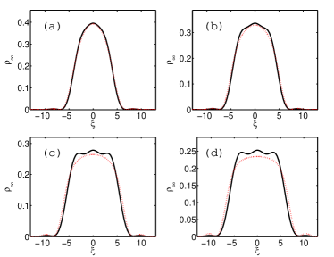
Figure 4: (color online) The asymptotic form of the SP density obtained exactly (black solid line), and with the hydrodynamic approach (red dotted line). The parameters used in the calculation are $N=3$, $L=\pi$, $c=1$ (a), $c=2$ (b), $c=5$ (c), and $c=10$ (d). (see text for details).

Let us follow upon our example from Section III, that is, let us consider the asymptotic form of the single particle density $\rho_{\infty}(\xi)$ of a LL gas which is initially in the ground state of a box with infinitely high walls; the length of the box is $L=\pi$. The calculation of the exact SP density demands performing multi-dimensional integration over $N-1$ variables which is not a simple task. For this reason, the number of particles in our calculation of the exact SP density is $N=3$. For the initial condition of the hydrodynamic approach $\psi_{H}(x,t=0)$ we could choose $\psi_{H}(x,t=0)=\sqrt{N/L}$ within the box, and zero otherwise. This would be a good initial condition in the thermodynamic limit (large $N$, $N/L=const.$). However, since for our exact calculation we used $N=3$, we have chosen, in order to be able to compare between the two approaches, the hydrodynamic initial field $\psi_{H}(x,t=0)=\sqrt{n_{\mathrm{exact}}}$, where $n_{\mathrm{exact}}$ is the exact SP density of the initial ground state (this can be calculated by employing Ref. Gaudin1971 ). Figure 4 displays the exact asymptotic form of the SP density, and the hydrodynamic asymptotic SP density. The latter is obtained numerically by solving Eq. (29) with the standard split-step Fourier technique; the nonlinear term in Eq. (29), that is, the function $f(c/|\psi_{H}(x)|^{2})$ is calculated by using values tabulated in Ref. [19] of Ref. Dunjko . The asymptotic dynamics in the hydrodynamic approach occurs after sufficiently long propagation, when the SP density starts exhibiting self-similar propagation (see also Ohberg2002 ).

The agreement is qualitatively excellent for all values of the interaction strength, and quantitatively excellent for $c<1$. The width of the SP density as a function of $\xi=x/t$ indicates the velocity of the expansion of the cloud. The asymptotic FWHM (full-width at half maximum) expansion velocity is in good agreement for all values of $c$. The hydrodynamic approximation does not reproduce small humps in the SP density, characteristic in the TG regime after expansion from the ground state; this discrepancy is expected to be smaller if we had calculated expansion from the ground state with large $N$, where the hydrodynamic approximation is expected to work even better.

Another possible comparison that can be made with the hydrodynamic approximation is the following. The LL wave function which is utilized as the initial condition in Sec. IV and Ref. Buljan2008 is obtained by acting with the operator $\hat{O}_{c}$ onto the fermionic ground state $\psi_{F0}$ in the harmonic trapping potential $V(x)=\nu^{2}x^{2}/4$. This wave function can approximate the ground state only when the commutator $[\hat{O}_{c},V(x)]$ can be neglected Buljan2008 . The SP density of this state can be compared with the static hydrodynamic density obtained in Ref. Dunjko for the LL gas in a harmonic trap. Due to the properties of the operator $\hat{O}_{c}$ Buljan2008 and the fermionic ground state in the harmonic trap $\psi_{F0}$, it is straightforward to verify that the shape of the SP density corresponding to the state $\hat{O}_{c}\psi_{F0}$ scales as $\rho(x)\rightarrow\rho(x/s)/s$ under the transformation $\nu\rightarrow\nu/s^{2}$, $c\rightarrow c/s$, that is, the shape of the SP density does not change under this transformation. The same is true for the shape of the (ground-state) SP density obtained with the hydrodynamic approach, which has been shown Dunjko to depend on a single parameter $\eta=(\frac{3N\nu}{4c^{2}})^{\frac{2}{3}}$ that is invariant under the transformation $\nu\rightarrow\nu/s^{2}$, $c\rightarrow c/s$. This is fully analogous to the case of a homogeneous LL gas where the only governing parameter $\gamma=c/n$ is invariant under a simultaneous rescaling of the interaction strength $c$ and the linear particle density $n$ Lieb1963 . The shape of the SP density of the state $\hat{O}_{c}\psi_{F0}$ (calculated for $N=3$) agrees with the shape obtained in Ref. Dunjko only in the Tonks-Girardeau limit ($\eta\ll 1$) where $\hat{O}_{c}\psi_{F0}$ is a good approximation for the ground state. If we reduce the interaction strength $c$ by keeping $\nu$ fixed, thereby increasing $\eta$, the two SP densities will no longer have a similar shape; this stems from a simple fact that $\hat{O}_{c}\psi_{F0}$ is an excited state for sufficiently small values of $c$, because the commutator $[\hat{O}_{c},V(x)]$ cannot be neglected, whereas the hydrodynamic solution approximates the ground state.

VII Conclusion

We have derived the asymptotic form of the wave function describing a freely expanding Lieb-Liniger gas. It is shown to have Tonks-Girardeau structure [see Eq. (15)], that is, the wave functions vanish when any two of the particle coordinates coincide. We have pointed out that the properties of these asymptotic states can significantly differ from the properties of a TG gas in a ground state of an external potential [see Fig. 1]. The dependence of the asymptotic state on the initial state is discussed [see Eq. (20)]. The analysis was performed for time-dependent Lieb-Liniger wave functions which can be obtained through the Fermi-Bose transformation (5). This encompasses initial conditions which correspond to the ground state of a repulsive Lieb-Liniger gas in physically realistic external potentials. Thus, our analysis characterizes the free expansion from such a ground state, after the potential is suddenly switched off. In deriving our main result, Eq. (15), we have used the stationary phase approximation. This generalizes and adds upon the result from Ref. Buljan2008 which was derived for a particular family of time-dependent Lieb-Liniger wave functions. We have demonstrated that the interaction energy of the freely expanding LL gas asymptotically decays according to a power law, $E_{\mathrm{int}}\propto t^{-3}$. Furthermore, we have calculated the asymptotic single-particle density for free expansion of a LL gas from an infinitely deep box potential. We have compared our exact calculation with the hydrodynamic approximation introduced in Ref. Dunjko , and employed in Ref. Ohberg2002 in the context of free expansion, obtaining good agreement for all values of the interaction strength. As a possible future avenue of research, we point out that the methodology employed here for the analysis of asymptotic wave functions has the potential to be exploited further to study the evolution of various observables (e.g., the momentum distribution which was studied for a TG gas Rigol2005 ) and correlations (e.g., see AMRey2008 and Refs. therein) during free expansion.

Appendix A Fermi-Bose transformation

In this appendix we outline the proof that the wave function (5) obeys both the cusp condition imposed by the interactions and Eq. (2), i.e., that it obeys Eq. (1). Without loss of generality we restrict our discussion to the fundamental permutation sector $R_{1}$. Let us write the differential operator as $\hat{O}_{c}=\prod_{1\leq i<j\leq N}\hat{B}_{ij}$, where

$$\hat{B}_{ij}=\left[1+\frac{1}{c}\left(\frac{\partial}{\partial x_{j}}-\frac{\partial}{\partial x_{i}}\right)\right].$$ (30)

We first show that the wave function (5) obeys the cusp condition (3) (see Ref. Korepin1993 ). Consider an auxiliary wave function

$$\psi_{\mathrm{AUX}}(x_{1},\ldots,x_{N},t) =\hat{B}_{j+1,j}\hat{O}_{c}\psi_{F}$$

$$=\hat{B}_{j+1,j}\hat{B}_{j,j+1}\hat{O}^{\prime}_{j,j+1}\psi_{F},$$ (31)

where the primed operator $\hat{O}^{\prime}_{j,j+1}=\hat{O}_{c}/\hat{B}_{j,j+1}$ omits the factor $\hat{B}_{j,j+1}$ as compared to $\hat{O}_{c}$. The auxiliary function can be written as

$$\psi_{\mathrm{AUX}}=\left[1-\frac{1}{c^{2}}\left(\frac{\partial}{\partial x_{j+1}}-\frac{\partial}{\partial x_{j}}\right)^{2}\right]\hat{O}^{\prime}_{j,j+1}\psi_{F}.$$ (32)

It is straightforward to verify that the operator $\hat{B}_{j+1,j}\hat{B}_{j,j+1}\hat{O}^{\prime}_{j,j+1}$ in front of $\psi_{F}$ is invariant under the exchange of $x_{j}$ and $x_{j+1}$. On the other hand, the fermionic wave function $\psi_{F}$ is fully antisymmetric with respect to the interchange of $x_{j}$ and $x_{j+1}$. Thus, $\psi_{\mathrm{AUX}}(x_{1},\ldots,x_{j},x_{j+1},\ldots,x_{N},t)$ is antisymmetric with respect to the interchange of $x_{j}$ and $x_{j+1}$, which leads to

$$\psi_{\mathrm{AUX}}(x_{1},\ldots,x_{j},x_{j+1},\ldots,x_{N},t)|_{x_{j+1}=x_{j}}=0.$$ (33)

This is fully equivalent to the cusp condition (3), $\hat{B}_{j+1,j}\psi_{B,c}|_{x_{j+1}=x_{j}}=0$. Thus, the wave function (5) obeys constraint (3) by construction.

Second, from the commutators $[\partial^{2}/\partial x_{i}^{2},\hat{O}_{c}]=0$ and $[i\partial/\partial t,\hat{O}_{c}]=0$ follows that if $\psi_{F}$ obeys Eq. (4), then $\psi_{B,c}$ obeys Eq. (2), which completes the proof.

If we use the expression

$$\hat{B}_{ij}=\left[\mathrm{sgn}(x_{j}-x_{i})+\frac{1}{c}\left(\frac{\partial}{\partial x_{j}}-\frac{\partial}{\partial x_{i}}\right)\right],$$ (34)

we obtain $\hat{O}_{c}=\prod_{1\leq i<j\leq N}\hat{B}_{ij}$ as in Eq. (6), which is valid inside any sector of the configuration space (see Gaudin1983 ). Note that for $c\rightarrow\infty$, one recovers Girardeau’s Fermi-Bose mapping Girardeau1960 , where the operator $\hat{O}_{c=\infty}=\prod_{1\leq i<j\leq N}\mbox{sgn}(x_{j}-x_{i})$ maps a noninteracting fermionic to a bosonic Tonks-Girardeau wave function.

References

-
(1)
E. Lieb and W. Liniger,
Phys. Rev. 130, 1605 (1963);
E. Lieb, Phys. Rev. 130, 1616 (1963). - (2) M. Girardeau, J. Math. Phys. 1, 516 (1960).
- (3) F. Schreck, L. Khaykovich, K.L. Corwin, G. Ferrari, T. Bourdel, J. Cubizolles, and C. Salomon, Phys. Rev. Lett. 87, 080403 (2001); A. Görlitz, J.M. Vogels, A.E. Leanhardt, C. Raman, T.L. Gustavson, J.R. Abo-Shaeer, A.P. Chikkatur, S. Gupta, S. Inouye, T. Rosenband, and W. Ketterle, ibid. 87, 130402 (2001); M. Greiner, I. Bloch, O. Mandel, T.W. Hansch, and T. Esslinger, ibid. 87, 160405 (2001); H. Moritz, T. Stöferle, M. Kohl, and T. Esslinger, ibid. 91, 250402 (2003); B. Laburthe-Tolra, K.M. O’Hara, J.H. Huckans, W.D. Phillips, S.L. Rolston, and J.V. Porto, ibid. 92, 190401 (2004); T. Stöferle, H. Moritz, C. Schori, M. Kohl, and T. Esslinger, ibid. 92, 130403 (2004).
- (4) T. Kinoshita, T. Wenger, and D.S. Weiss, Science 305, 1125 (2004); B. Paredes, A. Widera, V. Murg, O. Mandel, S. Fölling, I. Cirac, G. V. Shlyapnikov, T. W. Hänsch, and I. Bloch, Nature (London) 429, 277 (2004).
- (5) T. Kinoshita, T. Wenger, and D.S. Weiss, Nature (London) 440, 900 (2006).
- (6) M. Olshanii, Phys. Rev. Lett. 81, 938 (1998).
- (7) D.S. Petrov, G.V. Shlyapnikov, and J.T.M. Walraven, Phys. Rev. Lett. 85 3745 (2000).
- (8) V. Dunjko, V. Lorent, and M. Olshanii, Phys. Rev. Lett. 86 5413 (2001).
- (9) M. Gaudin, La fonction d’Onde de Bethe (Paris, Masson, 1983).
- (10) M.D. Girardeau, Phys. Rev. Lett. 91, 040401 (2003).
- (11) H. Buljan, R. Pezer, and T. Gasenzer, Phys. Rev. Lett. 100, 080406 (2008).
- (12) M.D. Girardeau and E.M. Wright, Phys. Rev. Lett. 84, 5691 (2000).
- (13) M.D. Girardeau and E.M. Wright, Phys. Rev. Lett. 84 5239 (2000).
- (14) P. Öhberg and L. Santos, Phys. Rev. Lett. 89, 240402 (2002); P. Pedri, L. Santos, P. Öhberg, and S. Stringari, Phys. Rev. A 68, 043601 (2003).
- (15) T. Busch and G. Huyet, J. Phys. B 36 2553 (2003).
- (16) M. Rigol and A. Muramatsu, Phys. Rev. Lett. 94, 240403 (2005); ibid. Mod. Phys. Lett. B 19, 861 (2005).
- (17) A. Minguzzi and D.M. Gangardt, Phys. Rev. Lett. 94, 240404 (2005).
- (18) A. del Campo and J.G. Muga, Europhys. Lett. 74, 965 (2006).
- (19) M. Rigol, V. Dunjko, V, Yurovskii, and M. Olshanii, Phys. Rev. Lett. 98, 050405 (2007).
- (20) H. Buljan, O. Manela, R. Pezer, A. Vardi, and M. Segev, Phys. Rev. A 74, 043610 (2006).
- (21) R. Pezer and H. Buljan, Phys. Rev. Lett. 98, 240403 (2007).
- (22) D.M. Gangardt and M. Pustilnik, Phys. Rev. A 77, 041604 (2008).
- (23) J.B. McGuire, J. Math Phys. (NY) 5, 622, (1964).
- (24) M. Gaudin, Phys. Rev. A 4, 386 (1971).
- (25) J.G. Muga and R.F. Snider, Phys. Rev. A 57, 3317 (1998).
- (26) K. Sakmann, A.I. Streltsov, O.E. Alon, and L.S. Cederbaum, Phys. Rev. A 72, 033613 (2005).
- (27) M.T. Batchelor, X.-W. Guan, N. Oelkers, and C. Lee, J. Phys. A 38, 7787 (2005).
- (28) Y. Hao, Y. Zhang, J.Q. Liang, and S. Chen, Phys. Rev. A 73, 063617 (2006).
- (29) A.D. Sykes, P.D. Drummond, and M.J. Davis, Phys. Rev. A 76, 063620 (2007).
- (30) R. Kanamoto, H. Saito, and M. Ueda, Phys. Rev. Lett. 94, 090404 (2005).
- (31) D.B. Creamer, H.B. Thacker, and D. Wilkinson, Phys. Rev. D 23, 3081 (1981).
- (32) M. Jimbo and T. Miwa, Phys. Rev. D 24, 3169 (1981).
- (33) V.E. Korepin, N.M. Bogoliubov, and A.G. Izergin, Quantum Inverse Scattering Method and Correlation Functions (Cambridge, Cambridge University Press, 1993).
- (34) T. Kojima, V.E. Korepin, N.A. Slavnov, Commun. Math. Phys. 188, 657 (1997)
- (35) M. Olshanii and V. Dunjko, Phys. Rev. Lett. 91, 090401 (2003).
- (36) D.M. Gangardt and G.V. Shlyapnikov, New J. of Phys. 5, 79 (2003).
- (37) G.E. Astrakharchik and S. Giorgini, Phys. Rev. A 68, 031602(R) (2003).
- (38) K.V. Kheruntsyan, D.M. Gangardt, P.D. Drummond, and G.V. Shlyapnikov, Phys. Rev. A 71, 053615 (2005).
- (39) P.J. Forrester, N.E. Frankel, and M.I. Makin, Phys. Rev. A 74, 043614 (2006).
- (40) J.-S. Caux, P. Calabrese, and N. A. Slavnov, J. Stat. Mech. (2007) P01008.
- (41) P. Calabrese and J.-S. Caux, Phys. Rev. Lett. 98, 150403 (2007).
- (42) M. Khodas, M. Pustilnik, A. Kamenev, and L.I. Glazman, Phys. Rev. Lett. 99, 109405 (2007).
- (43) G.P. Berman, F. Borgonovi, F.M. Izrailev, and A. Smerzi, Phys. Rev. Lett. 92, 030404 (2004).
- (44) W. Li, X. Xie, Z. Zhan, and X. Yang, Phys. Rev. A 72, 043615 (2005).
- (45) K.K. Das, M.D. Girardeau, and E.M. Wright, Phys. Rev. Lett. 89, 170404 (2002).
- (46) T. Cheon and T. Shigehara, Phys. Rev. Lett. 82, 2536 (1999).
- (47) V.I. Yukalov and M.D. Girardeau, Laser Phys. Lett 2, 375 (2005).
- (48) I. Bloch, J. Dalibard, and W. Zwerger, arXiv: 0704.3011v2 (2007).
- (49) P. Calabrese and J. Cardy, J. Stat. Mech. P06008 (2007).
- (50) M. Rigol, V. Dunjko, and M. Olshanii, Nature (London) 452, 854 (2008).
- (51) T.C. Dorlas, Commun. Math. Phys. 154 347 (1993).
- (52) L. Khaykovich, F. Schreck, G. Ferrari, T. Bourdel, J. Cubizolles, L. D. Carr, Y. Castin, C. Salomon, Science 296 1290 (2002).
- (53) H. Buljan, M. Segev, and A. Vardi, Phys. Rev. Lett. 95 180401 (2005).
- (54) A.I. Streltsov, O.E. Alon, and L.S. Cederbaum, Phys. Rev. Lett. 100 130401 (2008).
- (55) M.D. Girardeau, E.M. Wright, and J.M. Triscari, Phys. Rev. A 63, 033601 (2001).
- (56) E.B. Kolomeisky, T.J. Newman, J.P. Straley, and X. Qi, Phys. Rev. Lett. 85, 1146 (2000).
- (57) E. Toth, A.M. Rey, R.P. Blakie, arXiv:0803.2922 (2008).