The smallest free-electron sphere sustaining multipolar surface plasmon oscillation

Abstract

We study the oscillation frequencies and radiative decay rates of surface plasmon modes of a simple-metal sphere as a function of sphere radius without any assumptions concerning the sphere size. We re-examine within the framework of classical electrodynamics the usual expectations for multipolar plasmon frequency in the so called ”low radius limit” of the classical picture.

1 Introduction

The dielectric properties of metals, as well as those of semiconductors with high electron concentration, are due to collective effects arising from the Coulomb interaction between charges. In simple bulk metals the conduction electrons can be considered as a free-electron plasma. Frequency dependence of some of optical properties can be well described at a quantitative level by the Drude-Lorentz dielectric function  [1]. Optical properties of the electron gas in bulk metals, in proximity semi-infinitive surfaces, in thin films, and in metallic particles can be characterized by the eigenfrequencies of the system depending on free electron density and the geometry of the system. If we talk of ”plasmons” or ”plasma waves”, we mean eigenmodes of the self-consistent Maxwell equations for the system in the absence of an external electromagnetic field (or in a direction orthogonal to the field) (e.g. [2], [3]). ”Surface plasmons”, are used as a name for electromagnetic eigenmodes which are maximal near the surface. The time dependence of eigenmodes of a free-electron system is characterized by corresponding eigenfrequencies with the real part defining the frequency of oscillation, and the imaginary part defining the radiative damping.

Usually the eigenmode problem of a metallic sphere is studied in the limit of very small size parameter (retardation effect omitted), e.g. [4], [3], [5] and the radiative damping of plasmon oscillation is not included. The dipole mode eigenfrequency is then expected to be equal to $\omega_{p}/\sqrt{3}$ being responsible for the ”giant dipole resonance” resulting from the Mie scattering theory ([6], and also e.g. [7], [4], [8], [9]). $\omega_{p}$ is the modified plasma frequency, which can include or not the cluster core polarizability and (or) the spill-out effect of electron density at particle border, depending on the model approximations in effect.

In [10], [11] we have reconsidered the eigenvalue problem of a free-electron metal sphere as a function of sphere radius without any assumption concerning the particle size and including higher eigenmodes than the dipole ones. We have studied the dipole ($l=1$) and the higher polarity plasmon eigenfrequencies $\omega_{l}(R)$ as well as the plasmon radiative decay rates $\omega_{l}^{\prime\prime}(R)$ as a function of the particle radius $R$ with no assumption concerning the lower limit of the particle size in numerical modelling (retardation effects included) for $l=1,2,...6$. In [11] we have also studied the plasmon manifestation in scattering and absorbing properties of the sphere of arbitrarily large size (retardation included) within full scattering Mie theory.

In the present paper, we use the same ”exact” solutions of the eigenmode problem for $l=1,2,...6$ and $7,8...10$ in addition, and re-examine the usual expectation for multipolar plasmon frequencies in the so called ”low radius limit”. If the particle is formed from ideal metal (free electrons do not suffer from collisions $\gamma=0$) and is embedded in vacuum ($\varepsilon_{out}=1$) the multipolar plasmon frequencies according to the ”low radius limit” approximation are expected to be $\omega_{0,l}=\omega_{p}\sqrt{l/\left(2l+1\right)}$ (e.g. [12], [13], [3], [5]). The well known dipole mode frequency $\omega_{p}/\sqrt{3}$ is obtained for $l=1$, while for increasing $l$ the eigenmode frequencies approach the frequency of plane surface plasmon at $\omega_{p}/\sqrt{2}$, in spite of the fact they result from the ”low radius approximation” (i.e. from the limit of $R\rightarrow 0$, while plane surface limit is $R\rightarrow\infty$). In this paper we study the reasons of underlying causes for this paradox.

2 Formulation of the eigenvalue problem for a sphere of arbitrary size

The starting point is provided by the self-consistent Maxwell equations:

$$\begin{array}[]{cc}\nabla\times\mathbf{B}=\frac{1}{c^{2}}\frac{\partial\mathbf{E}}{\partial t}+\mu_{0}\mathbf{j}&\ \ \ \ \ \nabla\cdot\mathbf{E}=\rho/\varepsilon_{0}\\ \nabla\times\mathbf{E}=-\frac{\partial\mathbf{B}}{\partial t}&\ \ \ \nabla\cdot\mathbf{B}=0\end{array}$$ (1)

with no external sources: $\rho_{ext}=0$,$\ \mathbf{j}_{ext}=0$ so $\mathbf{j}$ and $\rho$ are induced current and charge densities respectively.

The frequency dependent dielectric function $\varepsilon(\omega)=\varepsilon_{in}(\omega)$ and conductivity $\sigma(\omega)=\sigma_{in}(\omega)$ of the sphere is assumed to have the constant bulk value up to the sphere border. The dynamic, linear response of the sphere material is described within standard optics, so the local proportionality between the electric displacement $\mathbf{D}$ and electric field intensity $\mathbf{\mathbf{E}}$ at the same point in space are valid: $\mathbf{D(\mathbf{r},\omega)=\mathbf{E}(\mathbf{r},\omega)}+\frac{i}{\omega}\mathbf{j}(\mathbf{r},\omega)=\varepsilon_{0}(1+\frac{i\sigma(\omega)}{\varepsilon_{0}\omega})\mathbf{E}(\mathbf{r},\omega)\mathbf{=}\varepsilon_{0}\varepsilon(\omega)\mathbf{E}(\mathbf{r},\omega)$. The sphere is embedded in nonconducting and nonmagnetic medium $\sigma_{out}=0$ and $\varepsilon(\omega)=\varepsilon_{out}$ will be assumed to be $\varepsilon_{out}=1$ in all numerical illustrations. The dielectric function of the sphere will be assumed to be the Drude dielectric function $\varepsilon_{in}(\omega)=1-\frac{\omega_{p}^{2}}{\omega^{2}-i\gamma\omega}$. We look for solutions fulfilling Maxwell’s equations in the form of transversal waves ($\nabla\cdot\mathbf{E}$ $=0$) in two homogeneous regions inside and outside the sphere so the wave equation: $\nabla^{2}\mathbf{E}(\mathbf{r})+\mathbf{\nabla}(\mathbf{\nabla}\cdot\mathbf{E}(\mathbf{r}))-\frac{1}{c^{2}}\frac{\partial^{2}\mathbf{D}}{\partial t^{2}}=0$ for harmonic fields $\mathbf{\mathbf{E}(\mathbf{r},\omega)=\mathbf{E}}e^{-i(kr-\omega t)}$ reduces to the Helmholtz equation:

$$\nabla^{2}\mathbf{E}(\mathbf{r})+q^{2}\mathbf{E}(\mathbf{r})=0$$ (2)

where: $q=q_{in}$ inside the sphere, $q=q_{out}$ in the sphere surroundings, $q_{in}=q_{0}\sqrt{\varepsilon_{in}}$ , $q_{out}=q_{0}\sqrt{\varepsilon_{out}}$ and $q_{0}=\frac{\omega}{c}$. The well known scalar solution of the corresponding scalar equation (e.g.[4], [8]) in spherical coordinates ($r,\theta,\phi$) reads:

$$\psi_{lm}(r,\theta,\phi)=Z_{l}(qr)Y_{lm}(\theta,\phi),$$ (3)

where $l=1,2,...,$ $m=0,\pm 1,...,\pm l$, $Y_{lm}(\theta,\phi)$ are spherical harmonics, and $Z_{l}(qr)$ are spherical Bessel functions $j_{l}(q_{in}r)$ inside the sphere and the spherical Hankel functions $h_{l}(q_{out}r)$ outside the sphere.

Because various notations have been employed in different papers and textbooks and none appears to have general acceptance, let’s recall that the spherical Bessel functions: $j_{l}\left(z\right)=\sqrt{\frac{\pi}{2z}}J_{l+\frac{1}{2}}(z),$ and $h_{l}\left(z\right)=j_{l}\left(z\right)-i\cdot n_{l}(z)=\sqrt{\frac{\pi}{2z}H_{l+\frac{1}{2}}^{(1)}(z)}$ where $n_{l}(z)=\sqrt{\frac{\pi}{2z}}N_{l+\frac{1}{2}}(z)$. The functions $J_{l+\frac{1}{2}}(z)$, $H_{l+\frac{1}{2}}^{\left(1\right)}(z)$ and $N_{l+\frac{1}{2}}(z)$ are Bessel, Hankel and Neuman cylindrical functions of half order of the standard type according to the convention used e.g. in [7].

From scalar solution $\psi_{lm}$ one can construct two independent solutions of the vectorial wave equation (2), one with vanishing radial component of the magnetic field:

$$\mathbf{E}(\mathbf{r}) = B_{lm}(1/q)\mathbf{\nabla\times\nabla\times(r}\psi_{lm}\mathbf{),}$$ (4)

$$\mathbf{H}(\mathbf{r}) = B_{lm}(q/iq_{0})\mathbf{\nabla\times(r}\psi_{lm}\mathbf{).}$$ (5)

and the other with vanishing radial component of the electric field:

$$\mathbf{E}(\mathbf{r}) = A_{lm}\mathbf{\nabla\times(r}\psi_{lm}\mathbf{),}$$ (6)

$$\mathbf{H}(\mathbf{r}) = A_{lm}(1/q_{0})\mathbf{\nabla\times\nabla\times(r}\psi_{lm}\mathbf{),}$$ (7)

$A_{lm}$ and $B_{lm}$ are constants that take different values $A_{lm}^{in}$ and $B_{lm}^{in}$ inside and $A_{lm}^{out}$ and $B_{lm}^{out}$ outside the sphere. The explicit expressions for the solution with the nonzero radial component of the electric field $E_{r}\neq 0$ (and the magnetic field tangent to the sphere surface $H_{r}=0)$, which is named transverse magnetic (TM) mode in analogy to the flat surface interface case (p polarization, or ”electric wave” in terminology of [7]) read:

$$E_{r}(r,\theta,\phi) = B_{lm}l(l+1)(qr)^{-1}Z_{l}(qr)Y_{lm}(\theta,\phi),$$

$$E_{\theta}(r,\theta,\phi) = B_{lm}(qr)^{-1}[qrZ_{l}(qr)]^{\prime}\partial Y_{lm}/\partial\theta,$$

$$E_{\varphi}(r,\theta,\phi) = B_{lm}im(qr\sin\theta)^{-1}[qrZ_{l}(qr)]^{\prime}Y_{lm}(\theta,\phi),$$

$$H_{r}(r,\theta,\phi) = 0,$$ (8)

$$H_{\theta}(r,\theta,\phi) = B_{lm}[\varepsilon(\omega)]^{1/2}(m/\sin\theta)Z_{l}(qr)Y_{lm}(\theta,\phi),$$

$$H_{\varphi}(r,\theta,\phi) = iB_{lm}[\varepsilon(\omega)]^{1/2}Z_{l}(qr)\partial Y_{lm}/\partial\theta,$$

The expression for the orthogonal solution with $E_{r}=0$ results from eqs.(6,7) (and is named transverse electric (TE) mode in analogy to the flat surface interface case (s polarization)). The prime indicates differentiation in respect to the argument, which is $q_{in}r$ or $q_{out}r$ correspondingly. We focus our attention on TM mode only.

The continuity relations at the sphere boundary for the tangential components of the electric field (the continuity of $E_{\theta}$ and $E_{\varphi}$) lead to the same condition:

$$B_{lm}^{in}(z_{B})^{-1}[z_{B}j_{l}(z_{B})]^{\prime}=B_{lm}^{out}(z_{H})^{-1}[z_{H}h_{l}(z_{H})]^{\prime}$$ (9)

while the tangential components of the magnetic field (the continuity of $H_{\theta}$ and $H_{\varphi}$) lead to the condition:

$$B_{lm}^{in}\sqrt{\varepsilon_{in}}j_{l}(z_{B})=B_{lm}^{out}\sqrt{\varepsilon_{out}}h_{l}(z_{H})$$ (10)

where:

$$z_{B}=q_{in}R=\frac{\omega}{c}R\sqrt{\varepsilon_{in}}$$ (11)

is the argument of the Bessel function $j_{l}$, and

$$z_{H}=q_{out}R=\frac{\omega}{c}R\sqrt{\varepsilon_{out}}=z_{B}\frac{\sqrt{\varepsilon_{out}}}{\sqrt{\varepsilon_{in}}}$$ (12)

is the argument of the Hankel function for $r=R$. The continuity relations for TM mode lead to non-trivial solutions (e.g. non-zero field amplitudes $B_{lm}$ inside and outside the sphere) only when:

$$\frac{[z_{B}j_{l}(z_{B})]^{\prime}}{\varepsilon_{in}j_{l}(z_{B})}=\frac{[z_{H}h_{l}(z_{H})]^{\prime}}{\varepsilon_{out}h_{l}(z_{H})}$$ (13)

We are interested in the properties of the sphere in the frequency regime of anomalous dispersion $\varepsilon_{in}(\omega)<0$. In that region only the TM eigenmodes exist, while the equation dispersion relation for TE mode has no solution for $\varepsilon_{in}(\omega)<0$ ([5] or [14]). $Z_{l}(qr)=j_{l}(q_{in}r)$ is then a function of a complex argument and the solutions given by eqs. (8) are called ”surface modes”. The fields are maximal at the sphere surface, with exception of the $l=1$ mode which is uniform throughout the sphere ([4] or [14]).

On writing down the dispersion relation for the TM mode (13) in terms of the more compact Riccati-Bessel function $\psi_{l}\left(z\right)=z\cdot j_{l}(z)$ and $\xi_{l}\left(z\right)=z\cdot h_{l}^{(1)}(z)$, the dispersion relation for the TM mode reads:

$$\sqrt{\varepsilon_{out}}\xi_{l}\left(z_{H}\right)\psi_{l}^{\prime}\left(z_{B}\right)-\sqrt{\varepsilon_{in}}\psi_{l}\left(z_{B}\right)\xi_{l}^{\prime}\left(z_{H}\right)=0$$ (14)

The boundary conditions are then satisfied only by a discrete set of characteristic complex values $z_{l}$ which are the roots of the complex function $D_{l}(z)\equiv\sqrt{\varepsilon_{out}}\xi_{l}\left(z_{H}(\omega)\right)\psi_{l}^{\prime}\left(z_{B}(\omega)\right)-\sqrt{\varepsilon_{in}(\omega)}\psi_{l}\left(z_{B}(\omega)\right)\xi_{l}^{\prime}\left(z_{H}(\omega)\right)$ of complex argument $z=z(\omega,R)$. Discretization of complex roots $z_{l}$ means the discretization of corresponding values $\omega=\Omega_{l}$, $l=1,2,3...$ which are allowed to be complex: $\Omega_{l}=\omega_{l}+i\omega_{l}^{\prime\prime}$. They define discrete eigenmode frequencies $\omega_{l}$ and damping rates $\omega_{l}^{\prime\prime}$ for the TM mode being the sum of corresponding components of (8) multiplied by $e^{i\Omega_{l}t}=e^{i\omega_{l}t}e^{\omega_{l}^{\prime\prime}t}$. The analytic form of $z_{l}=z_{l}(\Omega_{l}(R),R)$ is not known, nor the analytic form of the relation $\Omega_{l}(R)$. Let’s notice, that neither $z_{H}(\omega)$ nor $z_{B}(\omega)$ separately are appropriate to define the set of discrete characteristic values, contrary to what is suggested in [8].

We solved the dispersion relation (14) with respect to $\Omega_{l}$ numerically by treating the radius $R$ as an external parameter. Riccati-Bessel functions $\psi_{l}$, $\chi_{l}$ and $\xi_{l}$ (and their derivatives with respect to the corresponding arguments $z_{H}$ and $z_{B}$) were calculated exactly with use of the recurrence relation.

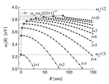
Figure 1: Plasmon oscillation frequencies $\omega_{l}(R)$ as a function of sodium sphere radius $R$ for $l=1,2,...10$ (rigorous solution). The picture illustrates the coincidence of the plasmon frequencies $\omega_{l}(R_{\min,l})$ with the corresponding value $\omega_{0,l}$ obtained within vanishing size approximation (open circles). $\gamma=0$.

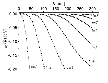
Figure 2: Rate of plasmon radiative damping $\omega_{l}^{\prime\prime}(R)$ as a function of sodium sphere radius $R$ for $l=1,2,...10$ resulting from non-approximated radius dependence for $\gamma=0$.

We have used the Mueller method of secants of finding numerical solutions of the function $f(v)=0$ when one knows the starting approximated values lying in the vicinity of the exact function parameter $v,$which can be complex (the ”root” function of the Mathcad program). For given $l$ and given $R$, the complex eigenvalue $\Omega_{l}$ was treated as the parameter to find, successive values of $R$ were external parameters and where changed with the step $\Delta R\approx 2$nm up to the final radius value $R=300$nm. The values for $\omega_{l}(R)$ and $\omega_{l}^{\prime\prime}(R)$ were searched for by starting from approximate values of the root procedure chosen from the range from $\omega_{p}\sqrt{3}$ up to $\omega_{p}\sqrt{2}$ correspondingly and for negative values of $\omega_{l}^{\prime\prime}$. The numerical illustrations have been made for a sodium sphere described by the Drude dielectric function with $\omega_{p}=5.6$ eV.

3 Results

Very careful study of roots of the function $D_{l}(\Omega_{l})$ of parameter $\Omega_{l}(R)$ for given $l$ for the decreasing limit of radii $R$ leads to the conclusion, that if the sphere is of the radius smaller than the characteristic radius $R_{\min,l}$, there exist no $\Omega_{l}(R)$ real nor complex. So the complex eigenfrequencies $\Omega_{l}(R)=\omega_{l}(R)+i\omega_{l}^{\prime\prime}(R)\$can be attributed to the sphere starting from the characteristic radius $R=R_{\min,l}\neq 0$ in given $l$. There exist no purely real solution for $\Omega_{l}$: surface plasmons are always damped, even if the dielectric function $\varepsilon(\omega)$ is real ($\gamma=0$).

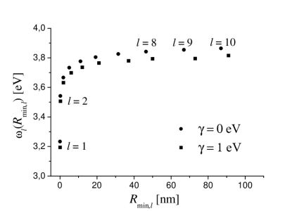
Figure 3: The relation of the plasmon frequency $\omega_{l}$ and $R_{\min,l}$ for successive values of $l=1,2,...10\$ for electron relaxation rates $\gamma=0$ and $\gamma=1$ eV

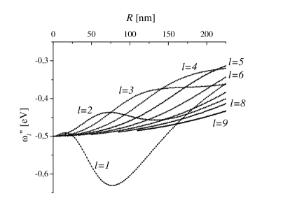
Figure 4: The dependence of damping rates: $\omega_{l}^{\prime\prime}(R)$ for the electron relaxation rate $\gamma=1$ eV for successive values of $l=1,2,...10$.

Figure 1 and 2 (solid lines with closed spheres) illustrate the obtained $\omega_{l}(R)$ and $\omega_{l}^{\prime\prime}(R)$ dependencies for $\gamma=0$ and $l=1,2,3,...10$ starting from $\omega_{l}(R_{\min,l})$ and $\omega_{l}^{\prime\prime}(R_{\min,l})$ values. These figures complete the picture for the $R\rightarrow R_{\min,l}$ limit of the corresponding dependence presented in [10], [11] for $l=1,2,...6$, figures 1 and 3, while in [10] we did not study the limiting case of $\omega_{l}(R\rightarrow R_{\min,l})$ nor $\omega_{l}^{\prime\prime}(R\rightarrow R_{\min,l})$ in detail. More careful search for these frequencies in the limit of smallest sphere still characterized by the eigenvalues $\omega_{l}(R_{\min,l})$ have shown, that they tend to the values which can be approximated by $\omega_{0,l}$ values:

$$\omega_{l}(R_{\min,l})\approx\omega_{0,l}=\omega_{p}\sqrt{\frac{l}{2l+1}},$$ (15)

as illustrated by the hollow circles in figure 1. Our numerical experiment shows that $R_{\min,l}$ dependence on $l$ can be described as $R_{\min,l}\approx C\left[l\left(2l+1\right)\right]^{3/2}$ with the proportionality constant $C$ depending on density of free electrons. $R_{\min,l}$ can be e.g.: $R_{\min,l=4}=6$nm, but it can be as large as $R_{\min,l=10}=87.2$nm (the size parameter $2\pi R/\lambda\simeq 1$ for optical wavelength $\lambda$).

The frequencies $\omega_{0,l}$ result from the dispersion relation (14) in the limit of small size parameter of the power series expansion of the spherical Bessel and Hankel functions.

$$j_{l}(z) = \frac{z^{l}}{(2l+1)!!}\left[1-\frac{0.5z^{2}}{1!(2l+3)}+....\right]$$ (16)

$$h_{l}(z) = -i\frac{(2l-1)!!}{z^{l+1}}\left[1-\frac{0.5z^{2}}{1!(1-2l)}+....\right]$$ (17)

where $(2l\pm 1)!!\equiv 1\times 3\times 5\times...\times(2l\pm 1)$. If one employs the widely used rough approximation (e.g.[3], [5], [14]):

$$\psi_{l}(z_{B}) \simeq \widetilde{\psi}_{l}(z_{B})=\frac{z_{B}^{l+1}}{(2l+1)!!},$$ (18)

$$\xi_{l}(z_{H}) \simeq \widetilde{\xi}(z_{H})=-i\frac{(2l-1)!!}{z_{H}^{l}},$$ (19)

the dispersion relation (14) is fulfilled for any radius $R$ of the sphere, and leads to the relation:

$$-\frac{l}{l+1}\frac{\varepsilon_{in}(\omega)}{\varepsilon_{out}}=1$$ (20)

giving discrete plasmon frequencies:

$$\omega_{0,l}=\omega_{p}\sqrt{\frac{l}{2l+1}}$$ (21)

which are real, in contrary to the exact solutions presented in figures 1 and 2 which are obligatory complex.

$\omega_{l}(R)$ dependence resulting from the exact solution do not smoothly tend to the value $\omega_{l}(R\rightarrow 0)$ with decreasing $R$, as usually expected (e.g.[3], [5], [10]), but it grows up to $\omega_{l}(R_{\min,l})$ value, as illustrated in figures 1. For $R<$ $R_{\min,l}$ there are no eigenvalues $\Omega_{l}(R)$. This behavior of the $\Omega_{l}(R)$ dependence is mainly due to fast divergence of the $\xi_{l}(z_{H})$ function entering the dispersion relation (14) for the arguments smaller than the range of variability of $z_{H}=z_{H}(\Omega_{l}(R),R)$ parameters for successive $l$.

When one includes the relaxation rate of the electron gas into the Drude model of the dielectric function, the plasmon frequency $\omega_{l}$ for given radius $R$ of the sphere is relatively slightly red shifted, while $\omega_{l}^{\prime\prime}$ experiences strong modification as illustrated in figure 3 and 4 respectively for $\gamma=1$ eV ([15]).

4 Conclusions

By carefully studying the radius dependence of eigenmode problem of a sphere one can formulate several conclusions allowing for better understanding of surface plasmon features. In this paper we concentrate on studying the differences of surface plasmon features in the classical picture resulting from treating the radius dependence exactly, and the expectations from the widely applied approximation of the so called ”low radius limit”. We use the example of sodium sphere of plasma frequency $\omega_{p}=5.6$ eV , however the conclusions are qualitatively valid for other simple free-electron metals. According to the non-approximated treatment the surface plasmons are always radiatively damped, even in the absence of collisional process: eigenfrequencies must be complex. The ”low radius limit” leads to the real eigenfrequencies $\omega_{0,l}$, which are radius independent. From the exact calculations one can conclude, that the radius dependence of multipolar plasmon frequencies is more subtle, than expected. Our calculations show, that at larger polarity the $\omega_{l}(R)$ dependence does not smoothly tend to the value $\omega_{0,l}=\omega_{p}\sqrt{l/\left(2l+1\right)}$ of the vanishing size limit, as one could expect (e.g.[12], [13]). If the sphere is of radius $R$ smaller than the characteristic radius $R_{\min,l}\sim\left[l\left(2l+1\right)\right]^{3/2}$, there is no related eigenvalue $\Omega_{l}(R)$ real nor complex. So the complex eigenfrequencies $\Omega_{l}(R)=\omega_{l}(R)+i\omega_{l}^{\prime\prime}(R)\$can be attributed to the sphere starting from the radius $R=R_{\min,l}\neq 0$. The radii $R_{\min,l}$ for higher polarities $l$ are not much smaller then the wavelength of the optical range (the anomalous dispersion range of alkalies) so the ”low limit approximation” loses its validity. Our ”numerical experiment” proves, that for the smallest particle radius $R_{\min,l}$ still possessing an eigenfrequency in given polarity $l$, the plasmon oscillation frequencies can be well approximated by the corresponding value resulting from the ”low radius limit” approximation: $\omega_{l}(R_{\min,l})\approx\omega_{p}\sqrt{l/\left(2l+1\right)}$. Even though the problem of the optical properties of metal sphere is at least as old as Mie theory [6], it seems, that the limitation for the smallest cluster still enabling the plasmon oscillations has not been discussed previously.

This work was partially supported by the Polish State Committee for Scientific Research (KBN), grant No. 2 P03B 102 22.

References

- [1] Ch. Kittel, Introduction to Solid State Physics, 7th Ed., Wiley, (1996).
- [2] H. Raether, Excitation of Plasmons and Interband Transitions by Electrons, in Springer Tracts in Modern Physics, vol.88 (1980)
- [3] F. Forstmann, R..R. Gerhardts, Metal Optics Near the Plasma Frequency, in Festkörperprobleme (Advances in Solid State Physics), vol.XXII, (1982) p.291
- [4] C. F. Bohren, D. R. Huffman, Absorption and Scattering of Light by Small Particles, Wiley, New York, 1983.
- [5] R. Rupin, in Electromagnetic Surface Modes, ed. A. D. Boardman, Wiley, Chichester, 1982
- [6] G. Mie, Ann. Phys. 25 (1908) 377
- [7] M. Born, E. Wolf, Principles of Optics, Pergamon, Oxford 1975.
- [8] J. A. Stratton, Electromagnetic Theory, McGraw-Hill Book Company, 1941
- [9] U. Kreibig, M. Vollmer, Optical Properties of Metal Clusters, Springer, 1995
- [10] K. Kolwas, S. Demianiuk, M. Kolwas, J. Phys. B 29 (1996) 4761
- [11] K. Kolwas, S. Demianiuk, M. Kolwas, Appl. Phys. B 65 (1997) 63
- [12] J. C. Ashley, T. L. Ferrel, R. H. Ritchie, Phys. Rev. B 10 (1974) 554
- [13] A. D. Boardman, B. V. Paranjape, J. Phys. F 7 (1977) 1935
- [14] R. Fuchs , P. Halevi, Basic Concepts and Formalism of Spatial Dispertion, in Spatial Dispertion in Solids and Plasmas, ed. P. Halevi, North-Holland 1992
- [15] S. Demianiuk, K. Kolwas, J. Phys. B 34 (2001) 1651