Correlation effects in ultracold two-dimensional Bose gases

Abstract

We study various properties of an ultracold two-dimensional (2D) Bose gas that are beyond a mean-field description. We first derive the effective interaction for such a system as realized in current experiments, which requires the use of an energy dependent $T$-matrix. Using this result, we then solve the mean-field equation of state of the modified Popov theory, and compare it with the usual Hartree-Fock theory. We show that even though the former theory does not suffer from infrared divergences in both the normal and superfluid phases, there is an unphysical density discontinuity close to the Berezinskii-Kosterlitz-Thouless transition. We then improve upon the mean-field description by using a renormalization group approach and show how the density discontinuity is resolved. The flow equations in two dimensions, in particular, of the symmetry-broken phase, already contain some unique features pertinent to the 2D $XY$ model, even though vortices have not been included explicitly. We also compute various many-body correlators, and show that correlation effects beyond the Hartree-Fock theory are important already in the normal phase as criticality is approached. We finally extend our results to the inhomogeneous case of a trapped Bose gas using the local-density approximation and show that close to criticality, the renormalization group approach is required for the accurate determination of the density profile.

I Introduction

Low-dimensional systems play a unique role in the study of many-body effects. For example, the enhanced importance of thermal fluctuations prevents a two-dimensional (2D) system with a continuous symmetry to undergo spontaneous symmetry breaking at any nonzero temperature, thus preventing the presence of true long-range order. This property is elucidated in the Mermin-Wagner-Hohenberg theorem Mermin:66 ; Hohenberg:67 . Nonetheless, the system still exhibits interesting properties. In particular, the 2D $XY$ model undergoes a special type of phase transition into a state which is characterized by only algebraic long-range order instead. The underlying mechanism that drives the phase transition, known as the Berezinskii-Kosterlitz-Thouless (BKT) transition Bere:72 ; Kost:73 , is the unbinding of vortex-antivortex pairs. Due to its topological nature, such a phase transition is difficult to incorporate into the standard Ginzburg-Landau theory with a local order parameter. For the ultracold 2D Bose gas, the absence of Bose-Einstein condensation (BEC) requires the concept of a quasi-condensate to understand the existence of algebraic long-range order and superfluidity Popov:83 ; Shlyapnikov:00 ; Kagan:00 ; Stoof:02 ; Hutchinson:04 . Experiments in the field of ultracold atomic gases have recently reached this interesting 2D regime to allow for the direct observation of this phenomenon in a highly controllable environment Dalibard:05 ; Dalibard:06 ; Cornell:07 ; Dalibard:07 ; Phillips:08 . The observation of dislocations in the interference pattern of two condensates Walls:98 ; Devreese:98 ; Dalibard:05 ; Cornell:07 and the studies of the coherence properties Demler:06 ; Dalibard:06 , for example, have all agreed with the universal predictions of BKT theory. More experiments and numerical simulations have come to address also various nonuniversal properties specific to the atomic gases under consideration Dalibard:07 ; Dalibard:07b ; Krauth:07 ; Krauth:08 ; Blakie:08 .

To describe the low-dimensional Bose gas at nonzero temperatures, the usual approach of the Bogoliubov theory is plagued with infrared divergences. However, these divergences can be shown to occur due to a spurious contribution from the condensate phase fluctuations in the Bogoliubov approach and by removing these contributions we can arrive at a modified Popov theory, which is valid for any dimension and at all temperatures Stoof:02 . In this paper, we first study this modified Popov theory for the ultracold 2D Bose gas and show that it contains a density discontinuity above the BKT transition, close to the point where the quasicondensate density becomes nonzero. To improve upon the mean-field description, we next employ a renormalization group (RG) approach to take into account the quantum and thermal fluctuations more accurately, in particular in the normal phase, when the modified Popov theory reduces to Hartree-Fock theory. The RG theory developed for the ultracold three-dimensional (3D) Bose gas was shown to be quantitatively successful in addressing effects beyond mean-field Stoof:96 . Here, we derive the analogous 2D RG flow equations and find the surprising result that they show features which are very different from the 3D RG theory. We first show how various characteristics of a quasicondensate are manifested in this framework. We then interpret these unique features as precursors of the BKT physics, even though we have not taken topological defects into account explicitly. This is because the RG theory is derived from the full atomic quantum field $\psi(\textbf{x},\tau)$ and not from its phase alone Wetterich:08 . With the RG approach, the density correction to the Hartree-Fock theory indeed resolves the unphysical density discontinuity in the mean-field description. Furthermore, it agrees with the equation of state of the modified Popov theory already above the critical temperature, which shows that the latter has correctly included correlation effects beyond the Hartree-Fock description even in the normal phase.

The paper is organized as follows. In Sec. II, we discuss the exact form of the $T$-matrix for ultracold 2D gases as realized under current experimental conditions, since it determines the effective interaction of the 2D Bose gas. Next, in Sec. III, we present the mean-field results from the modified Popov theory, and point out that the Hartree-Fock theory becomes unstable already above the BKT transition, even though a solution to the Hartree-Fock equation of state exists at all temperatures. The discontinuity in the density close to the BKT transition that results from the modified Popov theory is deemed unsatisfactory, and in Sec. IV, we present the required RG theory to improve upon this result. We discuss various interesting features of the flow equations in two dimensions and compute various nonuniversal quantities of interest within this approach. While the RG approach resolves the density discontinuity of the mean-field equation of state, it remains incapable of capturing all the critical properties known from the BKT physics. We also compute various many-body correlators, and show how correlation effects beyond a mean-field picture show up in the normal phase close to criticality. In Sec. V, we extend our results to the case of a trapped Bose gas and compare them with the ideal gas. We end with some concluding remarks in Sec. VI.

II Effective interaction in the 2D regime

Even though we shall be interested in ultracold 2D Bose gases, in experiments with atomic alkali-metal gases the realization of such a system is achieved by restricting the motion of a trapped 3D gas onto a plane. For the quantum degenerate gas to be in the 2D regime, one needs to ensure that the motion along the tightly confining axial direction is frozen out. This condition is met if $k_{B}T,\mu\ll\hbar\omega_{z}$, where $k_{B}T$ is the thermal energy, $\mu$ is the chemical potential, and $\omega_{z}$ is the axial trapping frequency.

In the ultracold limit of the gases under consideration, the effective interaction is in the first instance determined by the three-dimensional two-body $T$-matrix. We therefore begin with considering the full two-body Hamiltonian $\hat{H}_{0}+\hat{V}$ in the center-of-mass coordinate frame, where the free Hamiltonian $\hat{H}_{0}$ is given by

$$\hat{H}_{0}=-\frac{\hbar^{2}}{m}\vartriangle_{\textbf{r}}-\frac{\hbar^{2}}{m}\vartriangle_{z}+\frac{1}{4}m\omega_{z}^{2}z^{2},$$ (1)

$m$ is the atomic mass, and $\hat{V}$ is the interaction potential modeled by a short-ranged delta function of strength $V_{0}$. The center-of-mass coordinate frame is spanned by the r-plane, which is taken to be homogenous, and the $z$-axis in the tightly-confining direction. We denote the eigenstates of $\hat{H}_{0}$ by $|\textbf{k},n\rangle$, which are given by the product of 2D plane waves $\langle\textbf{r}|\textbf{k}\rangle=e^{i\textbf{k}\cdot\textbf{r}}$ and one-dimensional oscillator functions $\langle z|n\rangle=\phi_{n}(z)$. The latter functions are defined in the standard form, $\phi_{n}(z)=(2\pi)^{-1/4}(2^{n}n!\,l)^{-1/2}H_{n}(z/\sqrt{2}l)\exp(-z^{2}/4l^{2})$, where $l=\sqrt{\hbar/m\omega_{z}}$ is the harmonic length in the axial direction and $H_{n}(z)$ is the Hermite polynomial.

The Lippmann-Schwinger equation for the two-body $T$-matrix is given by

$$\hat{T}(E^{+})=\hat{V}+\hat{V}\frac{1}{E^{+}-\hat{H}_{0}}\,\hat{T}(E^{+}),$$ (2)

where $E^{+}=E+i0$ and the effective interaction in the 2D regime is given by the matrix element with respect to the axial ground state, i.e.,

$$T_{00}(E)\equiv\langle\textbf{k},n=0|\hat{T}(E)|\textbf{k}^{\prime},n=0\rangle.$$ (3)

By inserting the completeness relation $\sum_{n}\int d\textbf{k}|\textbf{k},n\rangle\langle\textbf{k},n|/(2\pi)^{2}=1$, the operator equation in Eq. (2) can be written as

$$\frac{1}{T(E)} = \frac{1}{V_{0}}-\sum_{n=0}^{\infty}\int\frac{d^{2}\textbf{k}}{(2\pi)^{2}}\frac{|\phi_{n}(0)|^{2}}{E-E_{0}(\textbf{k},n)},$$ (4)

where $T(E)$ is the matrix element with respect to 3D plane waves, which is related to the desired quantity $T_{00}(E)$ by means of $T_{00}(E)=|\phi_{0}(0)|^{2}T(E)$. Moreover, $E_{0}(\textbf{k},n)$ are the eigenvalues of the free Hamiltonian

$$E_{0}(\textbf{k},n)=2\epsilon_{\textbf{k}}+\left(n+\frac{1}{2}\right)\hbar\omega_{z},$$ (5)

with $\epsilon_{\textbf{k}}=\hbar^{2}\textbf{k}^{2}/2m$.

As it stands, Eq. (4) suffers from an ultraviolet divergence due to the delta function interaction potential, which neglects any momentum dependence at high momentum. To cure this divergence, we observe that while the harmonic oscillator functions with odd $n$ vanish at the origin, the functions with even $n$ have the asymptotic behavior

$$|\phi_{2n}(0)|^{2}=\frac{1}{\pi l\sqrt{2}}\frac{\Gamma(n+\frac{1}{2})}{\Gamma(n+1)}\sim\frac{1}{\pi l\sqrt{2n}}+{\cal O}\,\left(\frac{1}{n^{3/2}}\right),$$ (6)

for large quantum numbers $n$, where $\Gamma(n)$ denotes the Gamma function. It then follows that, for large $n$, the second term on the right-hand side of Eq. (4) takes the form

$$\int\frac{d^{2}\textbf{k}dk_{z}}{(2\pi)^{3}}\frac{1}{E-2\epsilon_{\textbf{k}}-2\epsilon_{k_{z}}},$$ (7)

with $k_{z}\equiv\sqrt{2n}/l$. This form diverges in the ultraviolet in exactly the same manner as the two-body $T$-matrix in the homogenous three-dimensional space, i.e., as

$$\frac{1}{T^{2B}(E)} = \frac{1}{V_{0}}-\int\frac{d^{3}\textbf{q}}{(2\pi)^{3}}\frac{1}{E-2\epsilon_{\textbf{q}}},$$ (8)

with $\textbf{q}=(\textbf{k},k_{z})$. On physical grounds, this behavior is expected since the short-distance behavior of the gas is not altered by the harmonic confinement and a standard renormalization procedure can therefore be implemented. The latter is achieved by eliminating the bare coupling strength $V_{0}$ in favor of the relevant physical parameter $T^{2B}(E\simeq 0)=4\pi\hbar^{2}a/m$ for the low-energy scattering, where $a$ is the 3D scattering length. After the elimination, a well-defined expression for the $T$-matrix,

$$\frac{1}{T(E)} = \frac{m}{4\pi\hbar^{2}a}-\sum_{n=0}^{\infty}\int\frac{d^{2}\textbf{k}}{(2\pi)^{2}}\frac{|\phi_{n}(0)|^{2}}{E-E_{0}(\textbf{k},n)}$$ (9)

$$-\int\frac{d^{3}\textbf{q}}{(2\pi)^{3}}\frac{1}{2\epsilon_{\textbf{q}}},$$

that no longer contains any divergence is obtained. It is shown in the Appendix that the effective interaction can be further worked out to yield

$$T_{00}(E)=\frac{2\sqrt{2\pi}\hbar^{2}}{m}\,\frac{1}{l/a+F(E)},$$ (10)

with

$$F(E)=F_{0}\!+\!\frac{1}{\sqrt{2\pi}}\!\sum_{n=0}^{\infty}\!\frac{(2n-1)!!}{(2n)!!}\ln\!\left[\frac{4n+1}{4n-2E/\hbar\omega_{z}}\right]\!\!,$$ (11)

where $F_{0}\simeq-0.3508$, and for convenience energies are measured with respect to the zero-point energy $\hbar\omega_{z}/2$ of the axial ground state. This result can be compared with the previous work of Petrov et al. Shlyapnikov:01 , where a different approach has been adopted. Thus, we see that the interaction takes a quasi-2D form, even though the system is kinematically two dimensional. The $T$-matrix $T_{00}(E)$ interpolates between the form of the interaction for the 3D and 2D cases, where the former is a constant and the latter has a logarithmic energy dependence. For the trapped atomic gases of interest, the condition $l/a\gg 1$ is usually satisfied. Hence the effective interaction is often well approximated by $T_{00}(E)\simeq 2\sqrt{2\pi}a\hbar^{2}/ml\equiv g$. Nonetheless, the exact form of the $T$-matrix with an energy dependence will turn out to be important in the present work. In Fig. 1, we show $|T_{00}(E)|$ as a function of energy. Besides that the overall scale is set by $g$, there are zeros at energies $2n\hbar\omega_{z}$ corresponding to the harmonic oscillator states with even $n$, due to the divergence of the logarithmic function. Note again that we have subtracted the zero-point energy.

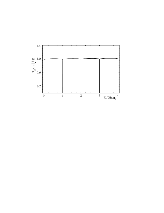
Figure 1: The exact $T$-matrix element $|T_{00}(E)|$ as a function of energy.

III Mean-Field Theory

In this section, we recapitulate the main result obtained from the modified Popov theory for the ultracold 2D Bose gas Stoof:02 . The equation of state in this mean-field theory is given by

$$n\negthickspace\! = \!\negthickspace n_{0}\!+\!\frac{1}{V}\!\sum_{\textbf{k}}\!\left\{\frac{\epsilon_{\textbf{k}}}{2\hbar\omega_{\textbf{k}}}\left[2N(\hbar\omega_{\textbf{k}})+1\right]\!-\!\frac{1}{2}\!+\!\frac{n_{0}T_{00}(-2\mu)}{2\epsilon_{\textbf{k}}+2\mu}\right\}$$ (12)

$$\equiv \!\negthickspace n_{0}\!+\!n^{\prime}$$

and $\mu=(2n-n_{0})\,T_{00}(-2\mu)$, where $n$ is the total density, $n_{0}$ is the (quasi)condensate density, $n^{\prime}$ is the density fluctuations around $n_{0}$, $\hbar\omega_{\textbf{k}}=[\epsilon^{2}_{\textbf{k}}+2n_{0}T_{00}(-2\mu)\epsilon_{\textbf{k}}]^{1/2}$ is the Bogoliubov quasiparticle dispersion, $N(x)=1/(e^{\beta x}-1)$ is the Bose-Einstein distribution function, and $\beta=1/k_{B}T$ is the inverse thermal energy. Notice that these equations do not suffer from infrared and ultraviolet divergences, and thus, they are valid for any dimension and at all temperatures. This comes about because the condensate phase fluctuations have been treated exactly to arrive at this result. A condensate with true long-range order is absent in two dimensions at any nonzero temperature. In fact, as shown in Ref. Stoof:02 , $n_{0}$ should be identified with the quasicondensate density at any nonzero temperature. Due to its mean-field nature, however, this equation of state is incapable to capture the BKT transition. Indeed, although the criterion for the BKT transition is $n_{s}\Lambda^{2}_{\textrm{th}}=4$, where $\Lambda_{\textrm{th}}=\sqrt{2\pi\hbar^{2}/mk_{B}T}$ is the thermal de Broglie wavelength of the atoms in the gas, according to Eq. (12), a nontrivial solution exists even if the superfluid density $n_{s}$ obeys $n_{s}\Lambda^{2}_{\textrm{th}}<4$. To circumvent this shortcoming, it was shown that by complementing the above equation of state with a renormalization group analysis on the Sine-Gordon model that takes into account vortices explicitly, the canonical criterion for the BKT transition is met when $n_{0}\Lambda^{2}_{\textrm{th}}=6.65$ Stoof:02 . Thus, above this critical temperature, the fugacity of the vortices renormalizes at long wavelengths to a nonzero value, which leads to the destruction of superfluidity but not immediately of the quasi-condensate.

The normal state without a quasicondensate is instead described by the Hartree-Fock equation of state given by

$$n=\frac{1}{V}\sum_{\textbf{k}}N(\epsilon_{\textbf{k}}+\hbar\Sigma-\mu),$$ (13)

where the Hartree-Fock self-energy $\hbar\Sigma$ satisfies

$$\hbar\Sigma=2nT_{00}(-\hbar\Sigma).$$ (14)

It is also noted that when the $T$-matrix is energy independent, i.e., $T_{00}(E)\simeq g$, the normal equation of state can actually be satisfied at all temperatures, since Eq. (13) can then be integrated to give

$$n\Lambda^{2}_{\textrm{th}}=-\ln(1-e^{-\beta(2ng-\mu)}).$$ (15)

For a fixed total density $n$, Eq. (15) has always a solution for the chemical potential $\mu$, at all temperatures. Thus to ensure the stability of the normal phase, we have to examine with the same chemical potential $\mu$ whether the solution of the modified Popov theory exists.

To illustrate this discussion, we numerically solve both equations of state, as shown in Fig. 2. We observe that there is an unphysical discontinuity in the density curve due to a mismatch in the total density between the two equations of state close to the BKT transition. This is an artifact of the mean-field theory which will be resolved in the next section.

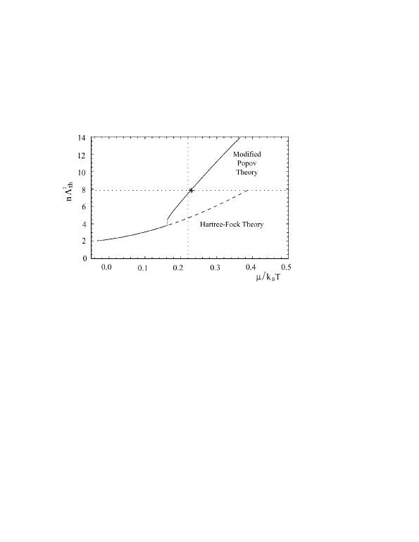
Figure 2: The mean-field equation of state from the modified Popov theory. The dashed curve is the Hartree-Fock theory that is extended also into the unstable regime until the Monte Carlo critical condition $n_{c}\Lambda_{\textrm{th}}^{2}=7.81$ is met (dotted line). We have taken $mg/\hbar^{2}=0.15$, which roughly corresponds to the experiment of Ref. Dalibard:05 . The canonical BKT criterion derived from the modified Popov theory is indicated with an asterisk.

To compare, we include in Fig. 2 the result from the usual Hartree-Fock mean-field approach. In this approach, the Hartree-Fock theory is employed up to a chemical potential that corresponds to the critical density $n_{c}$ obtained from the high precision Monte Carlo simulations Proko:01 . Numerical simulations yielded a critical density for the onset of the BKT transition of $n_{c}\Lambda^{2}_{\textrm{th}}\simeq\ln(380\,\hbar^{2}/mg)=7.81$, and a critical chemical potential $\mu_{c}/k_{B}T\simeq(mg/\pi\hbar^{2})\ln(13.2\,\hbar^{2}/mg)=0.22$, for $mg/\hbar^{2}\simeq 0.1541$. Both conditions are shown by the dotted lines in Fig. 2. It is noted that the critical chemical potential obtained within this mean-field approach, $\mu_{c}^{HF}/k_{B}T\simeq 0.38$, differs from the Monte-Carlo result, thus indicating an inconsistency in the Hartree-Fock approach. This can be understood within the modified Popov theory as an instability of the system toward a more correlated phase. On the other hand, despite the density discontinuity, the modified Popov theory yields a critical density $n_{c}^{MP}\Lambda^{2}_{\textrm{th}}\simeq 7.94$ and a critical chemical potential $\mu_{c}^{MP}/k_{B}T\simeq 0.23$, which are in excellent agreement with the Monte Carlo results. This shows that the main problem of the modified Popov theory lies in the inaccurate treatment of correlations in the region where it reduces to Hartree-Fock theory.

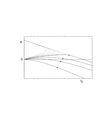
Figure 3: The RG flow diagram of $V_{0}$ and $\mu$ in the symmetric phase. The arrows indicate the flow direction towards the long-wavelength regime. The dotted lines are ill-defined trajectories as explained in the text.

IV Renormalization Group Theory

To improve upon the modified Popov theory, we employ here an RG approach Wilson:74 . In this approach, we systematically integrate out the high-momentum shell $\Lambda e^{-t}<k<\Lambda$, and absorb its contribution into the parameters of the theory, which then become dependent on the flow parameter $t$. Here, $\Lambda$ is the ultraviolet cutoff of the theory that is specified below. As discussed in Ref. Stoof:96 , due to the ultracold limit of the Bose gas under consideration, the parameters which are important in determining the various properties of interest are the chemical potential $\mu=\mu(t)$, and the two-body interaction strength $V_{0}=V_{0}(t)$.

IV.1 The Flow Equations

We shall present here the flow equations for these parameters in two dimensions, thus extending the results obtained in Refs. Stoof:96 ; note1 . In the symmetric phase, for $\mu<0$, the flow equations are given by

$$\frac{d\mu}{dt} = 2\mu-\frac{\Lambda^{2}}{\pi}V_{0}N(\epsilon_{\Lambda}-\mu),$$

$$\frac{dV_{0}}{dt} = -\frac{\Lambda^{2}}{2\pi}V_{0}^{2}\left[\frac{1+2N(\epsilon_{\Lambda}-\mu)}{2(\epsilon_{\Lambda}-\mu)}+4\beta N(\epsilon_{\Lambda}-\mu)\right.$$ (16)

$$\times[N(\epsilon_{\Lambda}-\mu)+1]\biggr{]},$$

while in the symmetry-broken phase, for $\mu>0$, they are

$$\frac{d\mu}{dt} = 2\mu-\frac{\Lambda^{2}}{2\pi}V_{0}\left[\frac{2\epsilon^{3}_{\Lambda}+6\mu\epsilon^{2}_{\Lambda}+\mu^{3}}{2\hbar^{3}\omega^{3}_{\Lambda}}[2N(\hbar\omega_{\Lambda})+1]-1\right.$$

$$\left.+\frac{\mu(2\epsilon_{\Lambda}+\mu)^{2}}{\hbar^{2}\omega^{2}_{\Lambda}}\beta N(\hbar\omega_{\Lambda})[N(\hbar\omega_{\Lambda})+1]\right],$$

$$\frac{dV_{0}}{dt} = -\frac{\Lambda^{2}}{2\pi}V_{0}^{2}\left[\frac{(\epsilon_{\Lambda}-\mu)^{2}}{2\hbar^{3}\omega^{3}_{\Lambda}}[2N(\hbar\omega_{\Lambda})+1]\right.$$ (17)

$$\left.+\frac{(2\epsilon_{\Lambda}+\mu)^{2}}{\hbar^{2}\omega^{2}_{\Lambda}}\beta N(\hbar\omega_{\Lambda})[N(\hbar\omega_{\Lambda})+1]\right].$$

Here, the chemical potential has been trivially rescaled by $\mu\rightarrow\mu e^{2t}$, hence the $2\mu$ term in the flow equations. The inverse temperature has also been trivially rescaled as $\beta\rightarrow\beta e^{-2t}$, but the interaction strength does not scale trivially in two dimensions. To examine the critical properties, however, a different trivial scaling needs to be used. This comes about because close to the critical regime, where the correlation length and correlation time diverge, the time-derivative term in the quantum action can be neglected with respect to the kinetic term. This is equivalent to taking the large-$t$ or high-temperature limit of the flow equations by setting $N(x)\rightarrow 1/\beta x$. As a result, while the trivial scaling of the chemical potential remains the same, the coupling strength acquires a trivial scaling with exponent 2, i.e., $V_{0}\rightarrow V_{0}e^{2t}$. As expected, the trivial scalings in the critical regime then agree with the trivial scalings of the classical $2D$ $XY$ model.

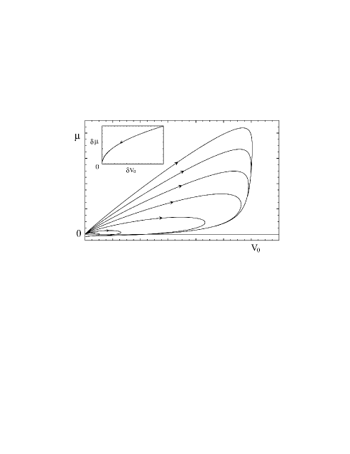
Figure 4: The RG flow diagram in the symmetry-broken phase. There is a limiting curve which ends at the attractor $(0,-\epsilon_{\Lambda}/2)$ where all trajectories approaches asymptotically. The inset shows the approach to the attractor.

To solve the flow equations, the correct boundary conditions have to be provided. The initial value for the chemical potential $\mu(t=0)$ is nothing but the bare chemical potential in the original theory. Its initial value can either be positive or negative, corresponding to an initial phase which is symmetry broken or unbroken, respectively. Furthermore, the flow equations allow the chemical potential to change sign, since the two sets of equations are smoothly connected at $\mu=0$. As we shall see, it is in fact a general feature of the solutions to the 2D flow equations in the symmetry-broken phase that the chemical potential always flows to a negative value for large $t$, which is not the case in three dimensions.

To determine the boundary condition for the interaction strength, we recognize that in vacuum, i.e., by setting $N(\epsilon_{\Lambda}-\mu)=0$, the flow equation for the interaction strength

$$\frac{dV_{0}}{dt}=-\frac{\Lambda^{2}}{2\pi}\frac{V_{0}^{2}}{2(\epsilon_{\Lambda}-\mu)}$$ (18)

is nothing but the differential form of the Lippmann-Schwinger equation for the $T$-matrix at energy $2\mu$. Since the $T$-matrix solution to the Lippmann-Schwinger equation, as obtained in Sec. II, entails the summation of all ladder diagrams for the scattering process in vacuum, we have to ensure that the flow equation in Eq. (18) reproduces the correct long-wavelength result for large $t$. In particular, the initial value $V_{0}(t=0)$ is chosen such that for large $t$ the correct form of the $T$-matrix is recovered in the vacuum, i.e., $V_{0}(t\rightarrow\infty)=T_{00}(2\mu)$. This can be satisfied by the following initial condition:

$$V_{0}(t=0)=\frac{2\sqrt{2\pi}\hbar^{2}}{m}\frac{1}{l/a+(1/\sqrt{2\pi})\ln\left(m\omega_{z}/2\hbar\Lambda^{2}\right)},$$ (19)

for $\hbar^{2}\Lambda^{2}/m\gg 2\mu$. It is important to note that for $\Lambda\gg\Lambda_{\textrm{th}}$, this procedure allows us to eliminate the ultraviolet cutoff dependence of the theory since the interaction strength already attained the two-body $T$-matrix value before entering the thermal regime Stoof:96 . With these boundary conditions and the ultraviolet cutoff chosen to be $\Lambda\sim{\cal O}\,(100\Lambda_{\textrm{th}})$, we now numerically integrate the flow equations to obtain the specific solution $\{V_{0}(t),\mu(t)\}$ for different chemical potentials.

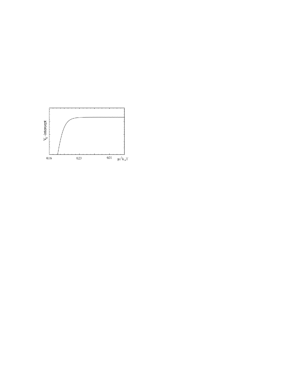
Figure 5: The intercept with the $V_{0}$ axis as a function of the chemical potential $\mu$.

IV.2 Analysis of the Flow Equations

We first study the two sets of flow equations in Eq. (IV.1) and Eq. (IV.1) separately, and allow for the chemical potential in both equations to take positive and negative values. In the symmetric phase, as seen in Fig. 3, the trajectories seem to be characteristics of the order-disorder phase transition of the classical 3D $XY$ model. The fixed point of the flow equations can be found by considering their large-$t$ limit

$$\frac{d\mu}{dt} = 2\mu-\frac{\Lambda^{2}V_{0}}{\pi}\frac{k_{B}T}{\epsilon_{\Lambda}-\mu}=0,$$

$$\frac{dV_{0}}{dt} = 2V_{0}-\frac{\Lambda^{2}V_{0}^{2}}{2\pi}\frac{5k_{B}T}{(\epsilon_{\Lambda}-\mu)^{2}}=0,$$ (20)

which yields $(V_{0}^{*},\mu^{*})=(20\pi\epsilon_{\Lambda}^{2}/49\Lambda^{2}k_{B}T,2\epsilon_{\Lambda}/7)$. However, it is important to note that for chemical potentials above a critical value, the resulting trajectories are actually ill-defined because $\mu(t)$ eventually grows to a point where the Bose-Einstein distribution diverges, i.e. $N(\epsilon_{\Lambda}-\mu)=\infty$. Thus, there is not really an order-disorder phase transition with increasing chemical potential. More generally, the first quadrant with positive chemical potential should be regarded as the unphysical region of the symmetric phase because the true minimum of the action is shifted away from the origin. Similarly, in three dimensions the unstable fixed point lying in this region does not give the most accurate critical properties of the system Stoof:96 .

In the symmetry-broken phase, the flow equations present a few rather surprising features, as shown in Fig. 4. First, all trajectories always flow into the fourth quadrant with a negative chemical potential. This feature can be interpreted as the prima facie property of a quasicondensate in two dimensions, where starting with an initial “condensate” $(\mu>0)$ at the shortest distance, as the high momentum shells are being integrated out, the symmetry always gets restored ($\mu<0$) in the infrared regime. In other words, the high-momentum fluctuations at long wavelength always destroy the coherence present at short distances.

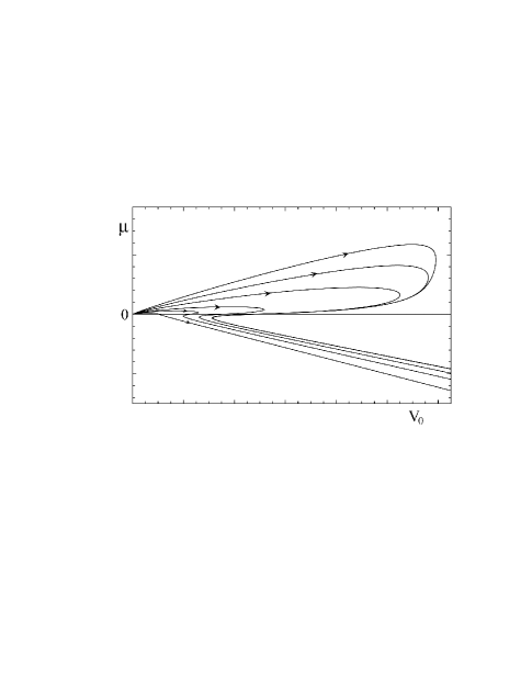
Figure 6: The RG flow diagram of the two sets of flow equations in the respective regions.

Second, there exists an attractor in the fourth quadrant towards which all the trajectories flow, without the need to fine tune the initial condition. The attractor can be found from solving the large-$t$ limit of the flow equations,

$$\frac{d\mu}{dt} = 2\mu-\frac{\Lambda^{2}V_{0}k_{B}T}{2\pi}\frac{2\epsilon_{\Lambda}^{3}+10\epsilon_{\Lambda}^{2}\mu+4\epsilon_{\Lambda}\mu^{2}+2\mu^{3}}{[\epsilon_{\Lambda}(\epsilon_{\Lambda}+2\mu)]^{2}}=0,$$

$$\frac{dV_{0}}{dt} = 2V_{0}-\frac{\Lambda^{2}V_{0}^{2}k_{B}T}{2\pi}\frac{5\epsilon_{\Lambda}^{2}+2\epsilon_{\Lambda}\mu+2\mu^{2}}{[\epsilon_{\Lambda}(\epsilon_{\Lambda}+2\mu)]^{2}}=0,$$ (21)

which give $(V_{0}^{*},\mu^{*})=(0,-\epsilon_{\Lambda}/2)$. Due to a non-analytic behavior of the differential equations near the attractor, an expansion of Eq. (IV.2) around the attractor $(V_{0}^{*}+\delta V_{0},\mu^{*}+\delta\mu)$ gives

$$\frac{d\delta\mu}{dt} \simeq -\epsilon_{\Lambda}+2\delta\mu+\frac{9\Lambda^{2}k_{B}T\epsilon_{\Lambda}}{32\pi}\frac{\delta V_{0}}{\delta\mu^{2}}$$

$$-\frac{15\Lambda^{2}k_{B}T}{16\pi}\frac{\delta V_{0}}{\delta\mu}-\frac{\Lambda^{2}k_{B}T}{8\pi\epsilon_{\Lambda}}\delta V_{0},$$

$$\frac{d\delta V_{0}}{dt} \simeq 2\delta V_{0}-\frac{9\Lambda^{2}k_{B}T}{16\pi}\frac{\delta V_{0}^{2}}{\delta\mu^{2}},$$ (22)

which thus does not permit a linearization. The approach to the attractor can nevertheless be found by substituting the ansatz $\delta V_{0}\propto 1/t^{2}$. In this manner we find that the direction of approach is given by

$$\delta\mu^{2}(t)\simeq\frac{9\Lambda^{2}k_{B}T}{32\pi}\frac{t}{1+t}\delta V_{0}(t),$$ (23)

and $\delta\mu\propto 1/t$ for large $t$. This is shown in the inset of Fig. 4.

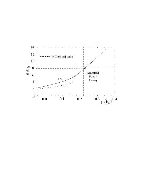
Figure 7: The RG equation of state, with $mg/\hbar^{2}=0.15$. The dashed lines are the critical conditions for the BKT transition from the Monte Carlo (MC) results. The dotted line is the modified Popov theory.

Third, there exists a limiting curve that all trajectories approach asymptotically. The intercept of the trajectories with the $V_{0}$ axis for increasing chemical potential is shown in Fig. 5. The interesting feature here is that for sufficiently large chemical potential the intercept essentially remains constant. We will come back to this point shortly.

Again, since the flow equations in the symmetry-broken phase are valid for $\mu>0$, the fourth quadrant should be considered as the unphysical region. However, the existence of an attractor and a limiting curve in the solution to the flow equations already suggests features which are unique to the ultracold 2D Bose gas, even though we did not take vortices into account explicitly. They are in fact related to the fixed line known from the BKT theory.

Finally, let us consider the system of coupled flow equations, and use the appropriate ones in the different quadrants. The result is shown in Fig. 6. The main point to note here is that a critical chemical potential $\mu_{c}$ can be identified for a fixed temperature, beyond which the resulting flow for large $t$ is insensitive to its initial value. This is so because for $\mu>\mu_{c}$, the trajectory changes the sign of $\mu(t)$ at essentially the same value of $V_{0}$, and thus the continuing flow into the fourth quadrant governed by the symmetric phase flow equations has essentially the same initial value. In other words, the long-wavelength action takes the same form for all $\mu>\mu_{c}$. As a result, we identify this $\mu_{c}$ with the critical condition for the BKT transition in this approach. It is interesting to note that the critical chemical potential obtained in this manner agrees within $10\%$ with the Monte Carlo result.

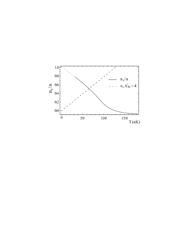
Figure 8: Superfluid fraction (solid curve) as a function of temperature for a density of $1.5\times 10^{9}\textrm{cm}^{-2}$, with $mg/\hbar^{2}=0.15$. The dotted line extrapolates the solid curve from the RG calculation to the lower temperature regime. The critical BKT condition is shown by the dashed line.

IV.3 RG Equation of State and Correlation Effects

Having discussed the properties of the flow equations, we next determine various nonuniversal quantities of interest. With the RG approach, the total density $n$ and the superfluid density $n_{s}$ can be computed by integrating these quantities along the trajectory, which are expressed by the following differential equations

$$\frac{dn}{dt} = \frac{\Lambda^{2}}{2\pi}\left[\frac{\epsilon_{\Lambda}+\mu}{2\hbar\omega_{\Lambda}}[2N(\hbar\omega_{\Lambda})+1]-\frac{1}{2}\right]e^{-2t},\textrm{ for }\mu>0,$$

$$\frac{dn}{dt} = \frac{\Lambda^{2}}{2\pi}N(\epsilon_{\Lambda}-\mu)e^{-2t},\textrm{ for }\mu<0,$$ (24)

and

$$\frac{dn_{s}}{dt}=\frac{dn}{dt}-\frac{\Lambda^{2}}{2\pi}\epsilon_{\Lambda}\beta N(x)\left[N(x)+1\right]e^{-2t},$$ (25)

where $x=\hbar\omega_{\Lambda}$ or $(\epsilon_{\Lambda}-\mu)$ for $\mu>0$ or $\mu<0$, respectively. The initial conditions are $n(t=0)=n_{s}(t=0)=0$. In Fig. 7, the density curve $n(t\rightarrow\infty)$ as a function of the chemical potential is shown and compared with the modified Popov theory. For small chemical potentials, the small deviation from the mean-field theory is consistent with the expectation that at low densities the RG correction is unimportant. As the chemical potential approaches the BKT critical point, however, the deviation from the Hartree-Fock theory becomes substantial. In fact, the RG density curve connects smoothly with the density curve obtained from the modified Popov theory. Thus, the RG approach resolves the artificial discontinuity observed in the mean-field theory. Furthermore, it shows that the equation of state for the quasi-condensate provides already a good description above the critical temperature.

Next, by integrating Eq. (25), the superfluid density is obtained, which is shown in Fig. 8. We see that the anticipated discontinuous jump in the superfluid density is absent at $n_{s}\Lambda_{\textrm{th}}^{2}=4$, which shows that not all universal features of the BKT transition are incorporated yet. We believe that the effects on the superfluid density associated with the proliferating vortices can be taken into account explicitly by performing an additional renormalization group analysis on the Sine-Gordon model, as done in Ref. Stoof:02 . The initial condition for the dielectric constant $K(0)=\beta\hbar^{2}n_{s}/m$ should then be identified with the superfluid density obtained here.

Finally, we compute various many-body correlators where enhanced correlation effects are expected to show up as criticality is approach. From the modified Popov theory, the renormalized density-density correlator is given by Stoof:02

$$K^{(2)}_{R}(T) \equiv \langle\hat{\psi}^{\dagger}(\textbf{x})\hat{\psi}^{\dagger}(\textbf{x})\hat{\psi}(\textbf{x})\hat{\psi}(\textbf{x})\rangle/2n^{2}$$ (26)

$$= \frac{1}{2n^{2}}\left[n_{0}^{2}+4n_{0}n^{\prime}+2(n^{\prime})^{2}\right].$$

The reduction in the three-body recombination is given by

$$\frac{L^{N}}{L(T)}\simeq\left\{\left[\frac{T_{00}(-2\mu)}{T_{00}(-2\hbar\Sigma)}\right]^{6}K_{R}^{(3)}(T)\right\}^{-1},$$ (27)

where $L^{N}$ is the recombination rate constant in the normal phase, and the renormalized three-body correlator is given by

$$K_{R}^{(3)}(T)=\frac{1}{6n^{3}}\left[n_{0}^{3}+9n_{0}^{2}n^{\prime}+18n_{0}(n^{\prime})^{2}+6(n^{\prime})^{3}\right].$$ (28)

In Fig. 9 and Fig. 10, we see that as the system in the normal phase approaches criticality, the mean-field description of Hartree-Fock theory for the many-body correlators breaks down completely. While the latter gives a constant value of 1 for the renormalized density-density correlator, the enhanced correlation due to the presence of a quasicondensate reduces this value to 0.68 at criticality. Furthermore, the three-body recombination rate reduces by a factor of 2.8, compared to the recombination rate constant in the normal phase. Thus, both these can serve as an observable for beyond Hartree-Fock effects.

Figure 9: Renormalized density-density correlator as a function of chemical potential, with $mg/\hbar^{2}=0.15$. The dotted line is the prediction from the Hartree-Fock theory, with $\langle n^{2}\rangle=2\langle n\rangle^{2}$. The dashed line is the BKT transition from the Monte Carlo result.

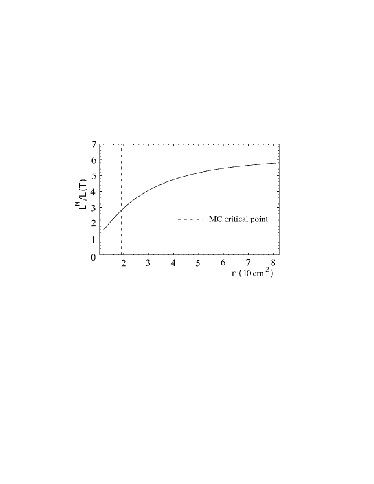
Figure 10: Reduction of the three-body recombination rate as a function of the density at temperature $T=84.4\textrm{ nK}$. The dashed line is the BKT transition from the Monte Carlo result.

V Trapped Bose Gases

In this section, we extend our results to the inhomogeneous case of trapped Bose gases. For the case of a trapped ideal Bose gas, the phenomenon of Bose-Einstein condensation (BEC) occurs. Within the local-density approximation (LDA), BEC takes place when the phase-space density in the center of the trap diverges. The temperature at which this phenomenon occurs, the BEC temperature $T_{BEC}$, can be related to the total particle number $N$ in the trap by Kleppner:91

$$N=\frac{\pi^{2}}{6}\left(\frac{k_{B}T_{BEC}}{\hbar\bar{\omega}}\right)^{2},$$ (29)

where $\bar{\omega}$ is the geometric mean of the radial trapping frequencies. For the case of a trapped interacting Bose gas in two dimensions, the system does not undergo a BEC, but a BKT transition if the trapping frequency $\bar{\omega}$ is sufficiently low Bhaduri:00 ; Baym:07 . For current experiments of interest, the harmonic length $\sqrt{\hbar/m\bar{\omega}}$ associated with the radial trapping frequencies easily exceeds the de Broglie wavelength $\Lambda_{\textrm{th}}$. Thus, the use of LDA by incorporating the effect of radial trapping through the introduction of a local chemical potential $\mu(r)=\mu-m\bar{\omega}^{2}r^{2}/2$ is readily justified. We show in Fig. 11 the density profile of an ideal Bose gas at the critical condition and compare it with the case of an interacting Bose gas within the LDA. Here, we see the drastic effect of interactions in the 2D Bose gas. For these conditions, the RG density profile for the interacting gas is only slightly different from the Hartree-Fock theory, which is stable in this case. We include the density profile of an ideal classical Boltzmann gas for comparison.

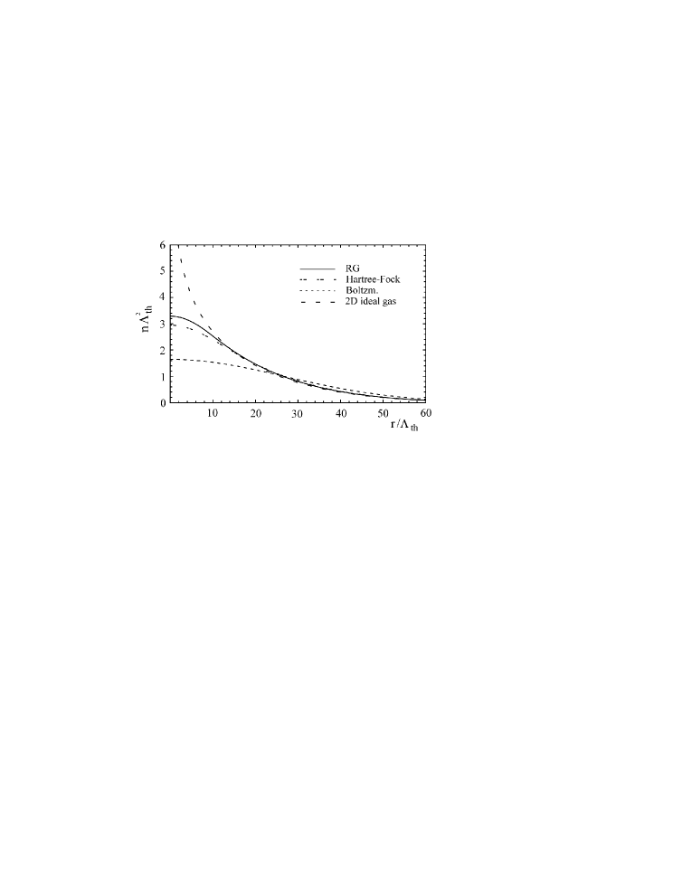
Figure 11: Density profiles for a quantum degenerate cloud of ${}^{87}\textrm{Rb}$ atoms for various theories for $N=7410$ at $T=T_{BEC}$. We take $a=5.2\textrm{nm}$, a radial trapping frequency of $\bar{\omega}=\sqrt{\omega_{x}\omega_{y}}=2\pi\sqrt{9.4\times 125}\textrm{ Hz}\simeq 2\pi\times 34.3\textrm{ Hz}$ and an axial trapping frequency $\omega_{z}=2\pi\times 4000\textrm{ Hz}$. With this particle number, the phase-space density in the center of the trap diverges for the ideal Bose gas.

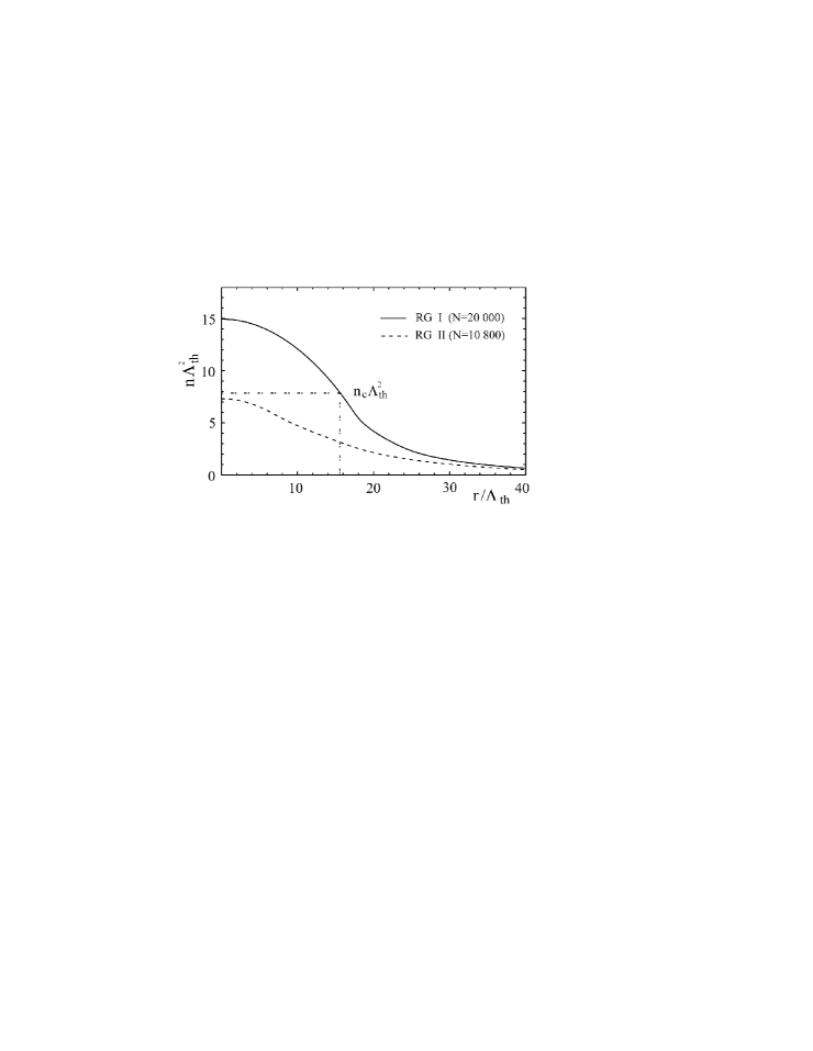
Figure 12: Density profiles from RG at $T=0.83\,T_{BEC}$ and $T=0.61\,T_{BEC}$, for $N=10800$ and $N=20000$, respectively. In this range of phase-space density, the Hartree-Fock theory is unstable towards the equation of state of the modified Popov theory. The dash-dotted line is the critical condition for the BKT transition.

As the phase-space density is increased, the Hartree-Fock theory is no longer applicable due to the instability towards a more correlated state with a quasicondensate, as discussed previously. We show the RG density profiles in this range of phase-space density in Fig. 12. The two density profiles describe two different regimes of the gas, namely, one with the phase-space density in the center of the trap slightly below the critical phase-space density $n_{c}\Lambda_{\textrm{th}}^{2}$ for the BKT transition, and the other well above it. We note that in the latter case, the gas consists of a superfluid core up to a critical radius, and is surrounded by an outer normal shell. One quantity of interest is the BKT transition temperature in the trap, relative to the ideal gas BEC temperature. By integrating the density profile at criticality, we obtain $T_{BKT}\simeq 0.81\,T_{BEC}$ for $mg/\hbar^{2}=0.15$.

There has been recent interesting experimental and numerical work Dalibard:07 ; Dalibard:07b ; Krauth:07 ; Krauth:08 ; Blakie:08 being carried out to address the nonuniversal quantities of the quasi-2D trapped Bose gases. A direct comparison with our theory is rendered difficult, because in these works, the thermal excitations in the tightly confining direction are non-negligible. Throughout our paper, we consider, instead, the strictly 2D regime, i.e., $\mu,k_{B}T\ll\hbar\omega_{z}$.

VI Conclusion

To conclude, we have studied various aspects of the 2D ultracold Bose gas. First, we derived the exact form of the $T$-matrix for the 2D system as realized in experiments. The 2D effective interaction assumes a form which interpolates between the 2D and 3D results. We then presented the mean-field results of the modified Popov theory. Even though the theory can describe both the normal and superfluid states, the density turns out to be discontinuous close to the BKT transition, which is an artifact of the theory. We improved upon the mean-field description by a RG approach. The flow equations exhibit interesting features, which resemble many of the unique properties of the 2D $XY$ model, even though the effects of vortices have not been included explicitly. With the RG approach, the density correction to the normal equation of state indeed connects smoothly with the quasicondensate equation of state in the superfluid phase. We then computed various many-body correlators in the normal phase close to criticality. We showed that deviations from the Hartree-Fock theory are important, and they show up in the renormalized density-density correlator and the reduction of the three-body recombination rate. We finally extended the results to the inhomogeneous case of trapped Bose gases. The density profiles for various phase-space densities were evaluated and we found that close to criticality, the RG approach becomes necessary for a quantitative description of the gas. We hope that these beyond mean-field effects can also be observed experimentally in the near future.

Appendix A

In this appendix we describe in detail the derivation of Eq. (10). Starting with Eq. (9), we add and subtract the quantity $\sum_{n}\int d^{2}\textbf{k}|\phi_{n}(0)|^{2}/(2\pi)^{2}E_{0}(\textbf{k},n)$ to obtain

$$\frac{1}{T(E)}=\frac{m}{4\pi\hbar^{2}a}+\frac{m}{4\pi\hbar^{2}}\sum_{n=0}^{\infty}|\phi_{2n}(0)|^{2}\ln\left[\frac{4n+1}{4n-2E/\hbar\omega_{z}}\right]+\sum_{n=0}^{\infty}\int\frac{d^{2}\textbf{k}}{(2\pi)^{2}}\frac{|\phi_{n}(0)|^{2}}{E_{0}(\textbf{k},n)}-\int\frac{d^{3}\textbf{q}}{(2\pi)^{3}}\frac{1}{2\epsilon_{\textbf{q}}},$$ (30)

where the zero-point energy $\hbar\omega_{z}/2$ has been subtracted from the energy argument $E$, and the integration

$$\int\frac{d^{2}\textbf{k}}{(2\pi)^{2}}\left[\frac{1}{E+\hbar\omega_{z}/2-E_{0}(2n,\textbf{k})}+\frac{1}{E_{0}(2n,\textbf{k})}\right]=\frac{m}{4\pi\hbar^{2}}\ln\left[\frac{4n+1}{4n-2E/\hbar\omega_{z}}\right]$$

has been carried out. The third term in the right-hand side of Eq. (30) can be written as

$$\sum_{n=0}^{\infty}\int\frac{d^{2}\textbf{k}}{(2\pi)^{2}}\frac{|\phi_{n}(0)|^{2}}{E_{0}(\textbf{k},n)} = \lim_{x\rightarrow 0}\sum_{n=0}^{\infty}\int\frac{d^{2}\textbf{k}}{(2\pi)^{2}}\frac{H_{2n}(0)H_{2n}(x/\sqrt{2}l)e^{-x^{2}/4l}}{\sqrt{2\pi}l2^{2n}(2n)!}\frac{1}{E_{0}(\textbf{k},2n)}$$ (31)

$$= \lim_{x\rightarrow 0}\int\frac{d^{2}\textbf{k}}{(2\pi)^{2}}\frac{e^{-x^{2}/4l}}{\sqrt{2\pi}l\hbar\omega_{z}}\sum_{n=0}^{\infty}\frac{(-1)^{n}H_{2n}(x/\sqrt{2}l)}{2^{2n}n!}\frac{1}{2n+\nu}$$

$$= \lim_{x\rightarrow 0}\int\frac{d^{2}\textbf{k}}{(2\pi)^{2}}\frac{e^{-x^{2}/4l}}{\sqrt{2\pi}l\hbar\omega_{z}}\sum_{n=0}^{\infty}\frac{L^{(-1/2)}_{n}(x^{2}/2l^{2})}{2n+\nu},$$

where the variable $\nu=1/2+l^{2}\textbf{k}^{2}$ is conveniently defined, $L^{(-1/2)}_{n}(x)$ is the generalized Laguerre function, and the relations $H_{2n}(0)=(-1)^{n}(2n)!/n!$ and $H_{2n}(x)=(-1)^{n}2^{2n}n!L_{n}^{(-1/2)}(x^{2})$ have been used.

Following Ref. Busch:98 , we use the integral representation

$$\frac{1}{2n+\nu}=\int_{0}^{\infty}dy\frac{1}{(1+y)^{2}}\left(\frac{y}{1+y}\right)^{2n+\nu-1}$$

for $2n+\nu>0$ and one of the generating functions of the generalized Laguerre function

$$\sum_{n=0}^{\infty}L_{n}^{(-1/2)}(x)z^{n}=(1-z)^{-1/2}\exp\left(\frac{xz}{z-1}\right).$$

In this manner we find

$$\sum_{n=0}^{\infty}\frac{L^{(-1/2)}_{n}(0)}{2n+\nu} = \int_{0}^{\infty}dy\frac{y^{\nu-1}(1+y)^{\nu-2}}{\sqrt{1+2y}}$$

$$= \frac{\pi^{2}2^{\nu-2}}{\Gamma(1-\nu/2)^{2}\Gamma(\nu)\sin^{2}(\pi\nu/2)}.$$

The last two terms in the right-hand side of Eq. (30) can then be numerically integrated to give

$$\negthickspace\negthickspace\negthickspace\negthickspace\negthickspace\sum_{n=0}^{\infty}\int\frac{d^{2}\textbf{k}}{(2\pi)^{2}}\frac{|\phi_{n}(0)|^{2}}{E_{0}(\textbf{k},n)}-\int\frac{d^{3}\textbf{q}}{(2\pi)^{3}}\frac{1}{2\epsilon_{\textbf{q}}}$$ (32)

$$= \frac{\pi^{3/2}}{4\sqrt{2}l\hbar\omega_{z}}\int\frac{d^{2}\textbf{k}}{(2\pi)^{2}}\frac{2^{\nu}}{\Gamma\left(1-\nu/2\right)^{2}\Gamma(\nu)\sin^{2}(\pi\nu/2)}$$

$$-\frac{m}{2\hbar^{2}}\int\frac{d^{2}\textbf{k}}{(2\pi)^{2}}\frac{1}{|\textbf{k}|}\simeq-0.0279\,\,m/l\hbar^{2}.$$

Finally, by using $T_{00}(E)=|\phi_{0}(0)|^{2}T(E)$, Eq. (10) is obtained.

References

- (1) N. D. Mermin and H. Wagner, Phys. Rev. Lett. 22, 1133 (1966).
- (2) P. C. Hohenberg, Phys. Rev. 158, 383 (1967).
- (3) V. L. Berezinskii, Sov. Phys. JETP 34, 610 (1972).
- (4) J. M. Kosterlitz and D. J. Thouless, J. Phys. C 6, 1181 (1973).
- (5) V. N. Popov, Theor. Math. Phys. 11, 565 (1972); Functional Integrals in Quantum Field Theory and Statistical Physics (Reidel, Dordrecht, 1983), Chap. 6.
- (6) D. S. Petrov, M. Holzmann, and G. V. Shlyapnikov, Phys. Rev. Lett. 84, 2551 (2000).
- (7) Yu. Kagan, V. A. Kashurnikov, A. V. Krasavin, N. V. Prokof ev, and B. V. Svistunov, Phys. Rev. A 61, 043608 (2000).
- (8) J. O. Andersen, U. Al Khawaja, and H. T. C. Stoof, Phys. Rev. Lett. 88, 070407 (2002); U. Al Khawaja, J. O. Andersen, N. P. Proukakis, and H. T. C. Stoof, Phys. Rev. A 66, 013615 (2002).
- (9) T. P. Simula, M. D. Lee, and D. A. W. Hutchinson, Phil. Mag. Lett. 85, 395 (2005).
- (10) S. Stock, Z. Hadzibabic, B. Battelier, M. Cheneau, and J. Dalibard, Phys. Rev. Lett. 95, 190403 (2005).
- (11) Z. Hadzibabic, P. Krüger, M. Cheneau, B. Battelier, and J. Dalibard, Nature 441, 1118 (2006).
- (12) V. Schweikhard, S. Tung, and E. A. Cornell, Rev. Lett. 99, 030401 (2007).
- (13) P. Krüger, Z. Hadzibabic, and J. Dalibard, Phys. Rev. Lett. 99, 040402 (2007).
- (14) P. Cladé, C. Ryu, A. Ramanathan, K. Helmerson, and W. D. Phillips, Phys. Rev. Lett. 102, 170401 (2009).
- (15) E. L. Bolda and D. F. Walls, Phys. Rev. Lett. 81, 5477 (1998).
- (16) J. Tempere and J. T. Devreese, Solid State Commun. 108, 993 (1998).
- (17) A. Polkovnikov, E. Altman, and E. Demler, Proc. Natl. Acad. Sci. USA 103, 6125 (2006).
- (18) Z. Hadzibabic, P. Krüger, M. Cheneau, S. P. Rath, J. Dalibard, New J. Phys. 10, 045006 (2008).
- (19) M. Holzmann and W. Krauth, Phys. Rev. Lett. 100, 190402 (2005).
- (20) M. Holzmann, M. Chevallier and W. Krauth, Europhys. Lett. 82, 30001 (2008).
- (21) R.N. Bisset, M.J. Davis, T.P. Simula, and P.B. Blakie, Phys. Rev. A 79, 033626 (2009).
- (22) M. Bijlsma and H. T. C. Stoof, Phys. Rev. A 54, 5084 (1996).
- (23) M. Gräter and C. Wetterich, Phys. Rev. Lett. 75, 378 (1995); G. V. Gersdorff and C. Wetterich, Phys. Rev. B 64, 054513 (2001); S. Floerchinger and C. Wetterich, Phys. Rev. A 79, 063620 (2009).
- (24) D. S. Petrov and G. V. Shlyapnikov, Phys. Rev. A 64, 012706 (2001).
- (25) N. Prokof’ev, O. Ruebenacker, and B. Svistunov, Phys. Rev. Lett. 87, 270402 (2001).
- (26) K. G. Wilson and J. Kogut, Phys. Rep. 12, 75 (1974).
- (27) For a detailed derivation of the flow equations, we refer the reader to Ref. Stoof:96 .
- (28) V. Bagnato and D. Kleppner, Phys. Rev. A 44, 7439 (1991).
- (29) R. K. Bhaduri, S. M. Reimann, S. Viefers, A. Ghose Choudhury, and M. K. Srivastava, J. Phys. B: At. Mol. Opt. Phys. 33, 3895 (2000).
- (30) M. Holzmann, G. Baym, J. -P. Blaizot, and F. Laloë, Proc. Nat. Acad. Sci. 104, 1476 (2007).
- (31) T. Busch, B. -G. Englert, K. Rzazewski, and M. Wilkens, Found. Phys. 28, 549 (1998).