Angular Diameters of the G Subdwarf $\mu$ Cassiopeiae A
and the K Dwarfs $\sigma$ Draconis and HR 511 from
Interferometric Measurements with the CHARA Array

Abstract

Using the longest baselines of the CHARA Array, we have measured the angular diameter of the G5 V subdwarf $\mu$ Cas A, the first such determination for a halo population star. We compare this result to new diameters for the higher metallicity K0 V stars, $\sigma$ Dra and HR 511, and find that the metal-poor star, $\mu$ Cas A, has an effective temperature ($T_{\rm eff}=5297\pm 32$ K), radius ($R=0.791\pm 0.008R_{\rm\odot}$), and absolute luminosity ($L=0.442\pm 0.014L_{\rm\odot}$) comparable to the other two stars with later spectral types. We show that stellar models show a discrepancy in the predicted temperature and radius for $\mu$ Cas A, and we discuss these results and how they provide a key to understanding the fundamental relationships for stars with low metallicity.

1 Introduction

Direct measurements of stellar angular diameters offer a crucial means of providing accurate fundamental information for stars. Advances in long baseline optical/infrared interferometry (LBOI) now enable us to probe the realm of cooler main-sequence stars to better define their characteristics. In their pioneering program at the Narrabri Intensity Interferometer, Hanbury Brown et al. (1974) produced the first modern interferometric survey of stars by measuring the diameters of 32 bright stars in the spectral type range O5 to F8 with seven stars lying on the main sequence. The current generation of interferometers possesses sufficiently long baselines to expand the main sequence diameter sensitivity to include even later spectral types, as exemplified by Lane et al. (2001), Ségransan et al. (2003), and Berger et al. (2006) who determined diameters of K$-$M stars and Baines et al. (2008) who measured the radii of exoplanet host stars with types between F7 and K0.

In this work, we focus primarily on the fundamental parameters of the well-known population II star $\mu$ Cassiopeiae ($\mu$ Cas; HR 321; HD 6582; GJ 53 A), an astrometric binary with a period of $\sim 22$ years consisting of a G5 + M5 pair of main sequence stars with low metallicity (Drummond et al. 1995, and references therein). With the CHARA Array, we have measured the angular diameter of $\mu$ Cas A to $<1\%$ accuracy, thereby yielding the effective temperature, linear radius, absolute luminosity and gravity (with accuracies of $0.6\%$, $1.0\%$, $3.2\%$, and $9.0\%$, respectively). We compare these newly determined fundamental stellar parameters for $\mu$ Cas A to those of two K0 V stars, HR 511 (HD 10780; GJ 75) and $\sigma$ Draconis ($\sigma$ Dra; HR 7462; HD 185144; GJ 764), which we also observed with the CHARA Array (§4.1). These fundamental parameters are then compared to model isochrones (§4.2).

2 Interferometric Observations

Observations were taken using the CHARA Array, located on Mount Wilson, CA, and remotely operated from the Georgia State University AROC facility in Atlanta, GA. The data were acquired over several nights using a combination of the longest projected baselines (ranging from 230$-$320 m) and the CHARA Classic beam combiner in $K^{\prime}$-band (ten Brummelaar et al. 2005). The data were collected in the usual calibrator-object-calibrator sequence (brackets), yielding a total of 26, 15, and 22 bracketed observations for $\mu$ Cas, $\sigma$ Dra, and HR 511, respectively.

For both $\mu$ Cas A and HR 511, we used the same calibrator star, HD 6210, which is a relatively close, unresolved, bright star with no known companions. Under the same criteria, we selected HD 193664 as the calibrator star for $\sigma$ Dra. For each star, a collection of magnitudes (Johnson $UBV$, Johnson et al. 1966; Strömgren $uvby$, Hauck & Mermilliod 1998; 2MASS $JHK$, Skrutskie et al. 2006) were transformed into calibrated flux measurements using the methods described in Colina et al. (1996), Gray (1998), and Cohen et al. (2003). We then fit a model spectral energy distribution (SED) to the observed flux calibrated photometry to determine the limb-darkened angular diameters $\theta_{\rm SED}$($T_{\rm eff}$, $\log g$) for these stars. We find $\theta_{\rm SED}$(6100, 3.8)=$0.519\pm 0.012$ mas for HD 6210 and $\theta_{\rm SED}$(6100, 4.5)=$0.494\pm 0.019$ mas for HD 193664. These angular diameters translate to absolute visibilities of 0.87 and 0.89 for the mean baselines used for the observations, or $\pm 0.8\%$ and $\pm 1.2\%$ errors, where these errors are propagated through to the final visibility measurements for our stars during the calibration process. An additional independent source of error is the uncertainty in the effective wavelength of the observed spectral bandpass. As described by McAlister et al. (2005), the effective wavelength of the $K^{\prime}$ filter employed for these observations has been adjusted to incorporate estimates of the transmission and reflection efficiencies of the surfaces and mediums the light encounters on its way to the detector, as well as for the effective temperature of the star. This calculation yields an effective wavelength for these observations of $2.15\pm 0.01\mu$m, which leads to a contribution at the $0.4\%$ level to the angular diameter error budget. Due to the fact that the flux distribution in the $K^{\prime}$-band for all of our stars is in the Rayleigh-Jeans tail, we find that there are no object-to-object differences in this calculation of effective wavelength due each star having a different effective temperature.

3 Data Reduction and Diameter Fits

The data were reduced and calibrated using the standard data processing routines employed for CHARA Classic data (see ten Brummelaar et al. 2005 and McAlister et al. 2005 for details). For each calibrated observation, Table 1 lists the time of mid-exposure, the projected baseline $B$, the orientation of the baseline on the sky $\psi$, the visibility $V$, and the 1-$\sigma$ error to the visibility $\sigma(V)$.

We did not detect the secondary star in $\mu$ Cas as a separated fringe packet (SFP) in any of our observations (see Farrington & McAlister 2006 for discussion on interferometric detections of SFP binaries). However, for close binaries, the measured instrumental visibility is affected by the flux of two stars, so in addition to our analysis of $\mu$ Cas A, we must account for incoherent light from the secondary star affecting our measurements. By calculating the ephemeris positions of the binary at the time of our observations, we get the separation $\rho_{\rm AB}$ of the binary during each observation. Although the most recent published orbital parameters are from Drummond et al. (1995), Gail Schaefer and collaborators (private communication) have provided us with their updated orbital elements for the binary based on Hubble Space Telescope observations taken every six months over the last decade. We use these separations (ranging from $1.380-1.396$ arcseconds) in combination with $\Delta M_{K}=3.5$ for the binary (McCarthy 1984) (assuming $K\approx K^{\prime}$) and seeing measurements at the time of each observation to calculate the amount of light the secondary contributes within our detector’s field of view (details described in Appendix  A). Fortunately our correction factors to the visibilities of $\mu$ Cas A are small ($0.4-1.4\%$), so even high uncertainties in this correction factor have minimal impact on the final corrected measurement.

In order to obtain limb-darkening coefficients for our target stars, SED fits were made to estimate $T_{\rm eff}$ and $\log g$. We used a bi-linear interpolation in the Claret et al. (1995) grid of linear limb-darkening coefficients in $K$-band ($\mu_{K}$) with our best fit SED parameters to get $\mu_{K}$ for each star. Because limb darkening has minimal influence in the infrared (here, we also assume $K\approx K^{\prime}$), as well as minimal dependence on temperature, gravity, and abundance for these spectral types, we feel that this method is appropriate and at most will contribute an additional one-tenth of one percent error to our limb-darkened diameters. We calculate the uniform-disk $\theta_{\rm UD}$ (Equation 1) and limb-darkened $\theta_{\rm LD}$ (Equation 2) angular diameters from the calibrated visibilities by $\chi^{2}$ minimization of the following relations (Brown et al. 1974):

$$V=\frac{2J_{1}(\rm x)}{\rm x},$$ (1)

$$V=\left({1-\mu_{\lambda}\over 2}+{\mu_{\lambda}\over 3}\right)^{-1}\times\left[(1-\mu_{\lambda}){J_{1}(\rm x)\over\rm x}+\mu_{\lambda}{\left(\frac{\pi}{2}\right)^{1/2}\frac{J_{3/2}(\rm x)}{\rm x^{3/2}}}\right],$$ (2)

and

$$\rm x=\pi\emph{B}\theta\lambda^{-1},$$ (3)

where $\emph{J}_{n}$ is the $n^{th}$-order Bessel function, and $\mu_{\lambda}$ is the linear limb darkening coefficient at the wavelength of observation. In Equation 3, B is the projected baseline in the sky, $\theta$ is the UD angular diameter of the star when applied to Equation 1 and the LD angular diameter when used in Equation 2, and $\lambda$ is the central wavelength of the observational bandpass.

The error to the diameter fit is based upon the values on either side of the minimum for which $\chi^{2}$ = $\chi^{2}_{\rm min}$ + 1 (Press et al. 1992; Wall & Jenkins 2003). A summary of these results is presented in Table 2, and Figures 1$-$2 show the best fits to our calibrated visibilities along with the 1-$\sigma$ errors.

4 Discussion

The linear radii, temperatures and absolute luminosities are calculated through fundamental relationships when the stellar distance, total flux received at Earth, and angular diameter are known. The linear radius of each star can be directly determined by combining our measured angular diameter with the Hipparcos parallax. Next, the fundamental relation between a star’s total flux $F_{\rm BOL}$ and angular diameter (Equation 4) is used to calculate the effective temperature $T_{\rm eff}$ and the absolute luminosity:

$$F_{\rm BOL}=\frac{1}{4}\theta_{\rm LD}^{2}\sigma T_{\rm eff}^{4},$$ (4)

where $\sigma$ is the Stefan-Boltzmann constant. For $\mu$ Cas A, $\sigma$ Dra, and HR 511, we calculate radii, effective temperatures, and luminosities purely from direct measurements (Table 2). For these calculations, the $F_{\rm BOL}$ for $\mu$ Cas A has been corrected for light contributed by the secondary by adopting the luminosity ratio of the two components from Drummond et al. (1995), effectively reducing its $F_{\rm BOL}$ by $1.3\%$.

Table 2 lists our derived temperatures for $\mu$ Cas A, $\sigma$ Dra, and HR 511 ($T_{\rm eff}=5297\pm 32,5299\pm 32$, and $5350\pm 76$ K, respectively). Our temperatures agree well with the numerous indirect techniques used to estimate $T_{\rm eff}$ with spectroscopic or photometric relationships. Temperatures of $\mu$ Cas A derived using these methods range from 5091$-$5387 K (5143$-$5344 K for $\sigma$ Dra and 5250$-$5419 K for HR 511), and while the internal error is low in each reference, the apparent discrepancy among the various methods shows that there is some systematic offset for each temperature scale, as might be expected if atmospheric line opacities are not correctly represented in the models.

4.1 Comparative Analysis to Observations of $\mu$ Cas A, $\sigma$ Dra, and HR 511

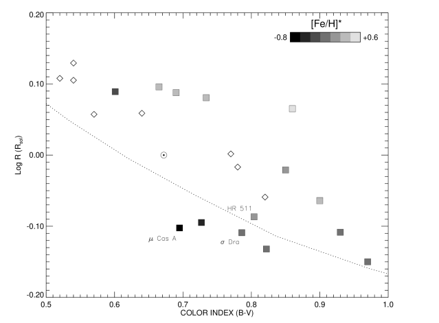
Figure 3: Plot of radius versus $B-V$ color index for G to mid-K type stars, including our results for $\mu$ Cas A, $\sigma$ Dra, and HR 511. Additional data plotted are from EB (diamonds, Andersen 1991), LBOI (squares, Baines et al. 2008, Kervella et al. 2004, and Lane et al. 2001), and the Sun ($\odot$). The grayscale legend indicates the metallicity estimates for LBOI points from Taylor (2005) (EB metallicity estimates are unreliable due to their duplicity). The dotted line represents a theoretical ZAMS line for solar metallicity (Y=0.275, Z=0.02) from the Dartmouth Stellar Evolution Models (Guenther et al. 1992; Chaboyer et al. 2001, available online at http://stellar.dartmouth.edu/).

It can be seen in Table 2 that the temperature, radius, and luminosity of $\mu$ Cas A is quite similar to that of $\sigma$ Dra and HR 511 despite the large difference in spectral types and $B-V$ color indices associated with the classical characteristics of metal-poor stars. These results support the conclusions in Drummond et al. (1995), where their model analysis predicts $\mu$ Cas A to have the characteristic radius, temperature, and luminosity of a typical K0 V star. In Figure 3, we compare our new linear radii versus $B-V$ color index to values measured from eclipsing binaries (EB’s) and other LBOI measurements, as well as the position of the Sun and a theoretical ZAMS for solar metallicity stars. The grayscale fill indicates metallicity estimates for the LBOI points, showing $\mu$ Cas A is currently the lowest metallicity star observed in this region of the HR diagram. The initial characteristics of evolution off the ZAMS is towards the upper-left region of the plot (larger and bluer), which is main reason for the dispersion of the stellar radii for stars in this region. ZAMS lines for sub-solar metallicities lie below this line, and are shifted to bluer colors.

Drummond et al. (1995) determine the mass of $\mu$ Cas A from the system’s astrometric orbital solution. Lebreton et al. (1999) update this mass utilizing the more accurate Hipparcos distance, yielding a mass of $0.757\pm 0.060$ $M_{\rm\odot}$. We use this mass with our new radius, to derive a directly measured surface gravity of $\log g=4.52\pm 0.04$. This value is comparable to the nominal values for solar metallicity ZAMS G5 V and K0 V stars being $\log g=4.49$ (Cox 2000).

We believe that the position of $\mu$ Cas A on Figure 3 does not come from underestimated errors in our data, or in the archival data. For instance, the uncertainty in the stellar radius can arise from the angular diameter we measure of the star (discussed in §3) and the Hipparcos parallax (Table 2). Because of their nearness to the Sun, the parallaxes of all three of our stars are well determined by Hipparcos, and with the combined accuracy of our angular diameters, the uncertainty on these radii are all less than $3\%$. The more pronounced discrepancy in the position of $\mu$ Cas A on Figure 3 is the large offset in the $B-V$ color index for $\mu$ Cas A with respect to the other two stars with the same effective temperatures, $\sigma$ Dra and HR 511. However, according to the ranking system of Nicolet (1978), all three stars we analyze have the highest quality index of photometry, with a probable error in $B-V$ of $\pm$0.006. In this catalog, the worst case scenario in photometry errors appears for characteristically dim stars with $V\gtrsim 10$, where the lowest rank quality index has an error in $B-V$ of $\pm$0.02, still not providing the desired effects to make the data agree within errors. With regards to the binarity of $\mu$ Cas A, the effect of the much cooler secondary star on the measured $B-V$ for the system as a whole would be less than one milli-magnitude (Casagrande et al. 2007), thus allowing us to ignore its contribution to these measurements as well. In other words, the position of $\mu$ Cas A on Figure 3 is simply a result of its lower metal abundance causing a reduction of opacity in its atmosphere, observationally making the star appear bluer in color than the other two stars with higher abundances with the same radius, effective temperature, and luminosity.

We would like to make it clear that for $\mu$ Cas A, a comparison of reduced opacities based solely on its iron abundance is a simplified approach, and complications arise in the determination of its true Helium abundance (Haywood et al. 1992) as well as enhanced $\alpha$-elements (Chieffi et al. 1991). In this respect, reducing the Helium abundance, or increasing the $\alpha$-element abundance, mimics the effect of increasing the metal abundance on a star’s effective temperature and luminosity. Additionally, over timescales of 10 Gyr, microscopic diffusion must also be considered in abundance analyses of subdwarfs (Morel & Baglin 1999). Here, we do not wish to misrepresent the impact of these issues on various stellar parameters and modeling, but instead present a purely observational comparison to fundamentally observed properties of these three stars. These topics will be discussed further in §4.2.

4.2 Stellar Models

While we can achieve a substantial amount of information from eclipsing binaries such as mass and radius, there still exists great uncertainty in the effective temperatures and luminosities of these systems (for example, see the discussion in §3.4 and §3.5 in Andersen 1991). On the other hand, while observing single stars with LBOI is quite effective in determining effective temperatures and luminosities of stars, it lacks the means of directly measuring stellar masses. For $\mu$ Cas A, the results of this work combined with our knowledge of the binary from previous orbital analysis provides us the best of both worlds. Unfortunately, the current uncertainty in mass for $\mu$ Cas A is $\sim 10\%$, too great to produce useful information about the star when running model evolutionary tracks (see discussion below, and Figure 7). However, our newly determined physical parameters of $\mu$ Cas A provide us with a handy way to test the accuracy of stellar models for metal poor stars.

To model $\mu$ Cas A, $\sigma$ Dra, and HR 511, we use both the Yonsei-Yale (Y²) stellar isochrones by Yi et al. (2001); Kim et al. (2002); Yi et al. (2003); Demarque et al. (2004), which apply the color table from Lejeune et al. (1998) and the Victoria-Regina (VR) stellar isochrones by VandenBerg et al. (2006) with $BVRI$ color-$T_{\rm eff}$ relations as described by VandenBerg & Clem (2003). To run either of these model isochrones, input estimates are required for the abundance of iron [Fe/H] and $\alpha$-elements [$\alpha$/Fe], both of which contribute to the overall heavy-metal mass fraction $Z$.

The atmosphere of $\mu$ Cas is metal poor, and there are numerous abundance estimates ranging from [Fe/H]=$-$0.98 (Fulbright 2000) to [Fe/H]=$-$0.55 (Clegg 1977), with the most recent estimates favoring lower metallicity values. Overall, this large range in metallicities suggests an error of $\Delta$[Fe/H]$\sim$0.2 dex. Systematic offsets aside, there exist a few additional variables which cause difficulties in determining accurate metallicity estimates for this star. Torres et al. (2002) argue that abundance estimates for a binary are affected by the presence of the secondary in both photometric and spectroscopic measurement techniques. However, Wickes & Dicke (1974) measured the system’s magnitude difference $\Delta$m$=5.5\pm 0.7$ at $\lambda$=0.55$\mu$m, limiting the secondary’s influence of these estimates to no more than $\Delta$[Fe/H]$\sim$0.05 dex, basically undetectable. Secondly, the abundance analysis by Thévenin & Idiart (1999) indicate that a careful non-LTE (NLTE) treatment is required when measuring stars with sub-solar abundances. In the case of $\mu$ Cas A, this correction factor is +0.14 dex, resulting in [Fe/H]${}_{NLTE}=-0.56$ from their measurements. Applying this correction factor brings the range of abundance estimates cited above to $-0.84<$[Fe/H]$<-0.41$.

In this work, we use the averaged metallicity values from the Taylor (2005) catalog for all three stars (Table 2). We caution the reader that this average value of [Fe/H] for $\mu$ Cas A, corrected for NLTE effects described above, still lies below the value from Thévenin & Idiart (1999) by about 0.12 dex; however, both of these estimates are within the range listed above. Lebreton et al. (1999) show that indeed these corrections are needed to remove a large part of the discrepancy on model fits to match observations. NLTE corrections for the iron abundance estimates of $\sigma$ Dra and HR 511 are not needed.

$\sigma$ Dra and HR 511 show no sign of $\alpha$-enhanced elements with respect to the Sun (i.e., [$\alpha$/Fe]=0), which is not a surprise because they have near solar iron abundances (Mishenina et al. 2004; Soubiran & Girard 2005; Fulbright 2000). However, these studies do detect the presence of $\alpha$-enhanced elements such as Ca, Mg, Si, and Ti in $\mu$ Cas A, and we adopt an average value from these three sources to be [$\alpha$/Fe]$=0.36\pm 0.06$.

To run models for each star, we round the average [Fe/H] value to the nearest [Fe/H] value in the VR models grids (Table 2), and adopt [$\alpha$/Fe]=0.3 for $\mu$ Cas A, and [$\alpha$/Fe]=0.0 for $\sigma$ Dra and HR 511. This approximation allows us to use identical input parameters in each of the models in order to compare the similarity of the models to each other (Figure 4). To justify this approximation, we ran the Y² models (using the interpolating routine available) for both the exact and rounded input parameters for $\mu$ Cas A and we were not able to see any substantial differences in comparing the two.

We show our results compared to the Y² (left column) and VR (right column) stellar isochrones in Figures 4$-$6 in both the temperature and color dependent planes. The sensitivity to age in this region is minimal, but for reference, we plotted 1, 5, and 10 Gyr isochrones for each model, as well as the positions of $\mu$ Cas A, $\sigma$ Dra and HR 511. When comparing the model isochrones for $\mu$ Cas A in Figure 4, no significant differences are seen between the Y² and VR models. However, for both models these results show that there exist discrepancies to observations in the $T_{\rm eff}$ plane. Both of the models overpredict the temperature for $\mu$ Cas A for a given luminosity and radius. On the other hand, on the color dependent plane, the models appear to do an adequate job fitting the observations in terms of luminosity (for a typical age of a halo star of $\sim$10 Gyr), but an offset is still seen in the model radii versus color index. In regards to model isochrones run for $\sigma$ Dra and HR 511 (Figures 5, 6), both of which have abundances more similar to the Sun, we find that the models and our observations agree quite well.

It is apparent in Figure 4 that although both of the models are fairly consistent with each other, the methods used to transform $B-V$ color index to $T_{\rm eff}$ for metal poor stars is not calibrated correctly. Likewise, as described by Popper (1997) as being a “serious dilemma,” several recent works (utilizing all the current measurements of stellar radii measured) show that models are infamous in predicting temperatures that are too high and radii that are too small, while still being able to correctly reproduce the stellar luminosity (e.g. Morales et al. 2008; Ribas et al. 2007; López-Morales 2007). Explanations for these discrepancies are understood to be a consequence of the stellar metallicity, magnetic activity, and/or duplicity.

In Figure 7, we show our observations dependent on stellar mass compared to the model Y² isochrones $\mu$ Cas A (VR models are not shown for clarity, but display approximately the same relations). Here it is clear that the current errors in the measured mass for $\mu$ Cas A is not sufficiently constrained to conclude anything useful from the models. Fundamental properties of the secondary star are also an important constraint within these parameters, especially in the respects of co-evolution of the binary, but unfortunately both the Y² and VR models do not extend to masses low enough to test these issues.

5 Conclusion

In this first direct measurement of the diameter of a subdwarf, we find that although $\mu$ Cas A is classified as a G5 V star, its sub-solar abundance leads it to resemble a K0 V star in terms of temperature, radius, and luminosity, whereas its surface gravity reflects the value for G5-K0 ZAMS stars with solar abundances. We find that while the both Y² and VR isochrones agree with our observations of $\sigma$ Dra and HR 511, a discrepancy is seen in temperature and radius when comparing these models to our observations of $\mu$ Cas A.

We are currently working on modeling this star and other subdwarfs with hopes to better constrain stellar ages and composition. Future plans to observe more stars of similar spectral types to determine angular diameters for main sequence stars are planned by TSB. This work will accurately determine the fundamental characteristics of temperature, radius, and absolute luminosity of a large sample of stars and thereby contribute to a broad range of astronomical interests.

Appendix A Appendix

We translate our measurement of the Fried parameter $r_{0}$ into the astronomical seeing disk $\theta_{\rm Seeing}$ by

$$r_{0}=1.009D\left(\frac{\lambda}{\theta_{\rm Seeing}D}\right)^{6/5}$$ (A1)

where $D$ is telescope aperture size, and $\lambda$ is wavelength of observation (ten Brummelaar 1993). To first order, an adequate representation of the intensity distribution of light from a star is a Gaussian (King 1971; Racine 1996), where $\theta_{\rm Seeing}$ is modeled as the full with at half maximum of the Gaussian . Thus, we can write the normalized intensity distribution of light for a star as

$$I(x,x_{0},y,y_{0})=\frac{1}{2\pi\sigma^{2}}\exp\left[{-\frac{1}{2\sigma^{2}}\left[(x-x_{0})^{2}+(y-y_{0})^{2}\right]}\right]$$ (A2)

where $\sigma\equiv 2.355^{-1}~{}\theta_{\rm Seeing}$, and the coordinates ($x_{0}$,$y_{0}$) determine the central position of the star on the chip. Assuming the primary star is at the center of our $2\times 2$ pixel array ($0,0$) and the secondary is offset by its separation in arcseconds ($0,\rho_{\rm AB}$), we then have the amount of light contributed by each star:

$$I_{A}=Q\int^{1}_{-1}\int^{1}_{-1}I(x,0,y,0)\,dx\,dy$$ (A3)

and

$$I_{B}=\int^{1}_{-1}\int^{1}_{-1}I(x,0,y,\rho_{\rm AB})\,dx\,dy$$ (A4)

with $Q$ being the intensity ratio of the two stars, $Q=10^{\Delta{\rm M_{K}}/2.5}$. Hence, the conversion of the measured visibility $V$ to the true visibility for the primary star $V_{A}$ is

$$V_{A}=V(1+I_{B}/I_{A}).$$ (A5)

Table 1: Interferometric Measurements

Star	JD	$B$	$\psi$	$V$	$\sigma(V)$
	($-$2,400,000)	(m)	(∘)
$\mu$ Cas A	54282.917	233.2	135.0	0.739	0.093
$\mu$ Cas A	54282.929	239.8	130.0	0.692	0.071
$\mu$ Cas A	54282.954	253.8	120.4	0.652	0.065
$\mu$ Cas A	54298.915	266.4	234.3	0.682	0.038
$\mu$ Cas A	54298.929	274.0	231.4	0.672	0.023
$\mu$ Cas A	54298.942	280.7	228.6	0.638	0.024
$\mu$ Cas A	54298.957	287.1	225.6	0.625	0.020
$\mu$ Cas A	54298.971	292.7	222.7	0.580	0.024
$\mu$ Cas A	54298.986	298.0	219.4	0.550	0.026
$\mu$ Cas A	54299.885	249.2	239.9	0.636	0.027
$\mu$ Cas A	54299.896	256.2	237.8	0.629	0.023
$\mu$ Cas A	54299.905	262.2	235.8	0.694	0.030
$\mu$ Cas A	54299.917	268.9	233.4	0.639	0.028
$\mu$ Cas A	54299.961	290.0	224.1	0.583	0.035
$\mu$ Cas A	54299.973	294.6	221.5	0.568	0.038
$\mu$ Cas A	54299.984	298.2	219.2	0.549	0.026
$\mu$ Cas A	54299.996	301.9	216.6	0.547	0.035
$\mu$ Cas A	54351.787	275.7	219.2	0.566	0.037
$\mu$ Cas A	54351.795	279.4	220.8	0.612	0.030
$\mu$ Cas A	54351.802	282.8	222.3	0.605	0.026
$\mu$ Cas A	54351.809	285.9	223.8	0.618	0.040
$\mu$ Cas A	54351.816	288.9	225.3	0.660	0.045
$\mu$ Cas A	54351.831	294.5	228.4	0.569	0.034
$\mu$ Cas A	54351.839	297.3	230.2	0.604	0.047
$\mu$ Cas A	54351.851	301.3	232.9	0.576	0.036
$\mu$ Cas A	54351.875	307.6	238.3	0.601	0.055
$\sigma$ Dra	54244.974	252.1	134.9	0.531	0.097
$\sigma$ Dra	54244.984	250.1	131.7	0.575	0.051
$\sigma$ Dra	54244.997	247.3	127.8	0.527	0.044
$\sigma$ Dra	54245.971	252.0	134.7	0.521	0.050
$\sigma$ Dra	54245.984	249.6	131.0	0.549	0.051
$\sigma$ Dra	54245.995	247.2	127.7	0.520	0.053
$\sigma$ Dra	54246.007	244.6	124.3	0.563	0.059
$\sigma$ Dra	54279.838	303.2	268.9	0.380	0.016
$\sigma$ Dra	54280.715	275.4	131.8	0.491	0.036
$\sigma$ Dra	54280.860	307.1	260.5	0.345	0.034
$\sigma$ Dra	54280.872	308.6	256.6	0.292	0.022
$\sigma$ Dra	54280.884	309.9	252.5	0.306	0.020
$\sigma$ Dra	54281.725	278.4	127.1	0.394	0.034
$\sigma$ Dra	54282.675	267.4	145.5	0.472	0.056
$\sigma$ Dra	54282.687	270.1	140.5	0.433	0.048
HR 511	52922.857	235.2	137.4	0.890	0.092
HR 511	52922.867	233.3	140.4	0.947	0.076
HR 511	54280.952	256.8	138.4	0.730	0.063
HR 511	54280.979	266.4	127.5	0.738	0.043
HR 511	54301.903	230.1	248.9	0.834	0.037
HR 511	54301.913	236.4	246.2	0.879	0.053
HR 511	54301.924	242.5	243.4	0.819	0.054
HR 511	54301.935	248.7	240.5	0.802	0.062
HR 511	54301.946	254.3	237.7	0.758	0.056
HR 511	54301.957	259.4	235.0	0.780	0.035
HR 511	54301.968	264.5	232.2	0.787	0.062
HR 511	54301.979	269.0	229.5	0.783	0.072
HR 511	54301.989	273.2	226.8	0.856	0.058
HR 511	54302.000	276.9	224.2	0.824	0.059
HR 511	54383.935	313.2	220.9	0.742	0.059
HR 511	54383.943	312.8	223.7	0.694	0.069
HR 511	54383.950	312.5	226.2	0.614	0.059
HR 511	54383.958	312.1	228.7	0.688	0.071
HR 511	54383.971	311.3	233.2	0.627	0.045
HR 511	54384.017	308.5	249.0	0.692	0.078
HR 511	54384.025	308.1	251.6	0.582	0.145
HR 511	54384.031	307.8	253.9	0.708	0.077

Table 2: Stellar Parameters

Element	$\mu$ Cas A	$\sigma$ Dra	HR 511
Spectral Type	G5 Vp	K0 V	K0 V
$V$ mag	05.17	04.70	05.63
$B-V$	00.69	00.79	00.81
$\pi_{hip}$ (mas)	$132.42\pm 0.60$00	$173.40\pm 0.46$00	$100.24\pm 0.68$00
$\theta_{\rm UD}$ (mas)	$0.951\pm 0.009$	$1.224\pm 0.011$	$0.747\pm 0.021$
Reduced $\chi^{2}_{\rm UD}$	0$0.96$	0$1.00$	0$0.78$
$\theta_{\rm LD}$ (mas)	$0.973\pm 0.009$	$1.254\pm 0.012$	$0.763\pm 0.021$
Reduced $\chi^{2}_{\rm LD}$	0$0.96$	0$1.01$	0$0.79$
Radius ($R_{\rm\odot}$)	$0.791\pm 0.008$	$0.778\pm 0.008$	$0.819\pm 0.024$
$F_{\rm BOL}$ (erg s-1 cm-2)	$2.482E-7$	$4.130E-7\tablenotemark{c}$	$1.588E-7$
$[$Fe/H$]$	.$-0.682$($-$0.71)	.$-0.199$($-$0.20)	00$0.005$(0.00)
$T_{\rm eff}$ (K)	$5297\pm 32$00	$5299\pm 32$00	$5350\pm 76$00
Luminosity ($L_{\rm\odot}$)	$0.442\pm 0.014$	$0.428\pm 0.013$	$0.49\pm 0.04$
$\log g$ (cgs)	$4.52\pm 0.04$	$\cdots$	$\cdots$

Figure 1: Limb-darkened angular diameter fit to $\mu$ Cas A.

Figure 2: Limb-darkened angular diameter fit to $\sigma$ Dra (bottom curve) and HR 511 (top curve).

Figure 4: $\mu$ Cas A data (along with 1-$\sigma$ errors) plotted against Y² and Victoria-Regina (VR) isochrones ([$\alpha$/Fe]=0.3, [Fe/H]=$-$0.71) for 1, 5, and 10 Gyr (solid, dotted, and dashed lines, respectively).

Figure 5: $\sigma$ Dra data (along with 1-$\sigma$ errors) plotted against Y² and Victoria-Regina (VR) isochrones ([$\alpha$/Fe]=0.0, [Fe/H]=$-$0.20) for 1, 5, and 10 Gyr (solid, dotted, and dashed lines, respectively).

Figure 6: HR 511 data (along with 1-$\sigma$ errors) plotted against Y² and Victoria-Regina (VR) isochrones ([$\alpha$/Fe]=0.0, [Fe/H]=0.00) for 1, 5, and 10 Gyr (solid, dotted, and dashed lines, respectively).

Figure 7: Mass relationships (along with 1-$\sigma$ errors) for $\mu$ Cas A compared to Y² isochrones for 1, 5, and 10 Gyr (solid, dotted, and dashed lines, respectively).

References

- Alonso et al. (1995) Alonso, A., Arribas, S., & Martinez-Roger, C. 1995, A&A, 297, 197
- Alonso et al. (1996) ——. 1996, A&AS, 117, 227
- Andersen (1991) Andersen, J. 1991, A&A Rev., 3, 91
- Baines et al. (2008) Baines, E. K., McAlister, H. A., ten Brummelaar, T. A., Turner, N. H., Sturmann, J., Sturmann, L., Goldfinger, P. J., & Ridgway, S. T. 2008, ArXiv e-prints, 803
- Bell & Gustafsson (1989) Bell, R. A., & Gustafsson, B. 1989, MNRAS, 236, 653
- Berger et al. (2006) Berger, D. H. et al. 2006, ApJ, 644, 475
- Blackwell & Lynas-Gray (1998) Blackwell, D. E., & Lynas-Gray, A. E. 1998, A&AS, 129, 505
- Brown et al. (1974) Brown, R. H., Davis, J., Lake, R. J. W., & Thompson, R. J. 1974, MNRAS, 167, 475
- Casagrande et al. (2007) Casagrande, L., Flynn, C., Portinari, L., Girardi, L., & Jimenez, R. 2007, ArXiv Astrophysics e-prints
- Chaboyer et al. (2001) Chaboyer, B., Fenton, W. H., Nelan, J. E., Patnaude, D. J., & Simon, F. E. 2001, ApJ, 562, 521
- Chieffi et al. (1991) Chieffi, A., Straniero, O., & Salaris, M. 1991, in Astronomical Society of the Pacific Conference Series, Vol. 13, The Formation and Evolution of Star Clusters, ed. K. Janes, 219
- Claret et al. (1995) Claret, A., Diaz-Cordoves, J., & Gimenez, A. 1995, A&AS, 114, 247
- Clegg (1977) Clegg, R. E. S. 1977, MNRAS, 181, 1
- Cohen et al. (2003) Cohen, M., Wheaton, W. A., & Megeath, S. T. 2003, AJ, 126, 1090
- Colina et al. (1996) Colina, L., Bohlin, R., & Castelli, F. 1996, HST Instrument Science Report, CAL/SCS-008 (Baltimore: STScI)
- Cox (2000) Cox, A. N. 2000, Allen’s astrophysical quantities (Allen’s astrophysical quantities, 4th ed. Publisher: New York: AIP Press; Springer, 2000. ed. Arthur N. Cox. ISBN: 0387987460)
- Demarque et al. (2004) Demarque, P., Woo, J.-H., Kim, Y.-C., & Yi, S. K. 2004, ApJS, 155, 667
- Drummond et al. (1995) Drummond, J. D., Christou, J. C., & Fugate, R. Q. 1995, ApJ, 450, 380
- Farrington & McAlister (2006) Farrington, C. D., & McAlister, H. A. 2006, in Presented at the Society of Photo-Optical Instrumentation Engineers (SPIE) Conference, Vol. 6268, Advances in Stellar Interferometry. Edited by Monnier, John D.; Schöller, Markus; Danchi, William C.. Proceedings of the SPIE, Volume 6268, pp. 62682U (2006).
- Fulbright (2000) Fulbright, J. P. 2000, AJ, 120, 1841
- Gray (1998) Gray, R. O. 1998, AJ, 116, 482
- Guenther et al. (1992) Guenther, D. B., Demarque, P., Kim, Y.-C., & Pinsonneault, M. H. 1992, ApJ, 387, 372
- Hanbury Brown et al. (1974) Hanbury Brown, R., Davis, J., & Allen, L. R. 1974, MNRAS, 167, 121
- Hauck & Mermilliod (1998) Hauck, B., & Mermilliod, M. 1998, A&AS, 129, 431
- Haywood et al. (1992) Haywood, J. W., Hegyi, D. J., & Gudehus, D. H. 1992, ApJ, 392, 172
- Johnson et al. (1966) Johnson, H. L., Iriarte, B., Mitchell, R. I., & Wisniewskj, W. Z. 1966, Communications of the Lunar and Planetary Laboratory, 4, 99
- Kervella et al. (2004) Kervella, P. et al. 2004, in IAU Symposium, Vol. 219, Stars as Suns : Activity, Evolution and Planets, ed. A. K. Dupree & A. O. Benz, 80
- Kim et al. (2002) Kim, Y.-C., Demarque, P., Yi, S. K., & Alexander, D. R. 2002, ApJS, 143, 499
- King (1971) King, I. R. 1971, PASP, 83, 199
- Lane et al. (2001) Lane, B. F., Boden, A. F., & Kulkarni, S. R. 2001, ApJ, 551, L81
- Lebreton et al. (1999) Lebreton, Y., Perrin, M.-N., Cayrel, R., Baglin, A., & Fernandes, J. 1999, A&A, 350, 587
- Lejeune et al. (1998) Lejeune, T., Cuisinier, F., & Buser, R. 1998, A&AS, 130, 65
- López-Morales (2007) López-Morales, M. 2007, ApJ, 660, 732
- McAlister et al. (2005) McAlister, H. A. et al. 2005, ApJ, 628, 439
- McCarthy (1984) McCarthy, Jr., D. W. 1984, AJ, 89, 433
- Mishenina et al. (2004) Mishenina, T. V., Soubiran, C., Kovtyukh, V. V., & Korotin, S. A. 2004, A&A, 418, 551
- Morales et al. (2008) Morales, J. C., Ribas, I., & Jordi, C. 2008, A&A, 478, 507
- Morel & Baglin (1999) Morel, P., & Baglin, A. 1999, A&A, 345, 156
- Nicolet (1978) Nicolet, B. 1978, A&AS, 34, 1
- Popper (1997) Popper, D. M. 1997, AJ, 114, 1195
- Press et al. (1992) Press, W. H., Teukolsky, S. A., Vetterling, W. T., & Flannery, B. P. 1992, Numerical recipes in C. The art of scientific computing (Cambridge: University Press, —c1992, 2nd ed.)
- Racine (1996) Racine, R. 1996, PASP, 108, 699
- Ribas et al. (2007) Ribas, I., Morales, J., Jordi, C., Baraffe, I., Chabrier, G., & Gallardo, J. 2007, ArXiv e-prints, 711
- Ségransan et al. (2003) Ségransan, D., Kervella, P., Forveille, T., & Queloz, D. 2003, A&A, 397, L5
- Skrutskie et al. (2006) Skrutskie, M. F. et al. 2006, AJ, 131, 1163
- Soubiran & Girard (2005) Soubiran, C., & Girard, P. 2005, A&A, 438, 139
- Taylor (2005) Taylor, B. J. 2005, ApJS, 161, 444
- ten Brummelaar (1993) ten Brummelaar, T. 1993, Ph.D. Thesis, University of Sydney
- ten Brummelaar et al. (2005) ten Brummelaar, T. A. et al. 2005, ApJ, 628, 453
- Thévenin & Idiart (1999) Thévenin, F., & Idiart, T. P. 1999, ApJ, 521, 753
- Torres et al. (2002) Torres, G., Boden, A. F., Latham, D. W., Pan, M., & Stefanik, R. P. 2002, AJ, 124, 1716
- VandenBerg et al. (2006) VandenBerg, D. A., Bergbusch, P. A., & Dowler, P. D. 2006, ApJS, 162, 375
- VandenBerg & Clem (2003) VandenBerg, D. A., & Clem, J. L. 2003, AJ, 126, 778
- Wall & Jenkins (2003) Wall, J. V., & Jenkins, C. R. 2003, Practical Statistics for Astronomers (Princeton Series in Astrophysics)
- Wickes & Dicke (1974) Wickes, W. C., & Dicke, R. H. 1974, AJ, 79, 1433
- Yi et al. (2001) Yi, S., Demarque, P., Kim, Y.-C., Lee, Y.-W., Ree, C. H., Lejeune, T., & Barnes, S. 2001, ApJS, 136, 417
- Yi et al. (2003) Yi, S. K., Kim, Y.-C., & Demarque, P. 2003, ApJS, 144, 259