Estimating Third-Order Moments for an Absorber Catalog

Abstract

Due to recent availability of large surveys, there is renewed interest in third-order correlation statistics. Measures of third-order clustering are sensitive to the structure of filaments and voids in the universe and are useful for studying large-scale structure. Thus statistics of these third-order measures can be used to test and constrain parameters in cosmological models.

Third-order measures such as the three-point correlation function are now commonly estimated for galaxy surveys. Studies on third-order clustering of absorption systems will complement these analyses. We define a statistic, which we denote as $\mathcal{K}$, that measures third-order clustering of a dataset of point observations, and focus on the estimation of this statistic for an absorber catalog. The statistic $\mathcal{K}$ can be considered a third-order version of the second-order Ripley’s $K$ function and allows one to study the abundance of various configurations of point triplets. In particular configurations consisting of point triplets that lie close to a straight line can be examined.

Studying third-order clustering of absorbers requires consideration of the absorbers as a three-dimensional process, observed on Quasi-stellar object (QSO) lines of sight that extend radially in three-dimensional space from the Earth. Since most of this three-dimensional space is not probed by the lines of sight, edge corrections become important. We use an analytical form of edge correction weights and construct an estimator of the statistic $\mathcal{K}$ for use with an absorber catalog. We show that with these weights, ratio-unbiased estimates of $\mathcal{K}$ can be obtained. Results from a simulation study also verify unbiasedness and provide information on the decrease of standard errors with increasing number of lines of sight.

1 Introduction

The C iv and Mg ii Quasi-stellar object (QSO) absorption systems or absorbers appear to trace the same structure as that of galaxies on very large scales and have been shown to be effective probes of large-scale structure in the universe (Crotts, 1985; Crotts et al., 1985; Tytler et al., 1993). See Tripp & Bowen (2005) for a discussion on the connection between galaxies and QSO absorbers using observations at low redshift.

The clustering of such absorbers were studied in a series of investigations (Vanden Berk et al., 1996; Quashnock et al., 1996; Quashnock & Vanden Berk, 1998) using an extensive catalog of absorbers drawn from the literature. Specifically, they performed a second-order correlation analysis in one dimension, restricting to absorber pairs lying on the same QSO lines of sight, and found clustering on very large scales, up to 50 to 100 $h^{-1}$Mpc. This superclustering has also been found in other studies, e.g. Heisler et al. (1989); Dinshaw & Impey (1996). This work on the second-order clustering of absorbers complements the analyses of second-order structure of other astronomical objects such as galaxies, quasars and the cosmic microwave background.

In astronomy, a common measure of second-order structure is the two-point correlation function $\xi$ (Peebles, 1980, 1993), and this is the function used in the above-mentioned studies. Another measure of second-order clustering is the reduced second moment function, also called Ripley’s $K$ function (Ripley, 1988; Martínez & Saar, 2002). In three dimensions, the $K$ function is related to the two-point correlation function by

$$K(r)=4\pi\int_{0}^{r}u^{2}[1+\xi(u)]\,du.$$

Martínez et al. (1998) applied the $K$ function to galaxy surveys, while Quashnock & Stein (1999); Stein et al. (2000) used it to examine clustering of the Vanden Berk et al. (1996) C iv absorber catalog.

Loh et al. (2001) extended the work of Quashnock & Stein (1999) in the study of second-order clustering of the Vanden Berk et al. (1996) absorber catalog by considering the absorbers as a process occurring in three dimensions. By treating the absorbers as a three-dimensional process, absorber pairs that lie on different lines of sight were included in estimates of the $K$ function. As a result, the estimates obtained were shown to have dramatically smaller standard errors than estimates obtained by only considering the absorbers as a one-dimensional process on the lines of sight, when there is a large enough number of lines of sight.

More recently, there has been interest in higher-order clustering, in particular in third-order clustering, partly because of limitations of restricting to second moments and partly because datasets are now large enough for third-order statistics to be estimated. In particular, the structure of filaments and voids that is present in galaxy surveys is more readily, though still inadequately, described by third-order statistics (Gaztañaga & Scoccimarro, 2005; Sefusatti & Scoccimarro, 2005). See Jing & Börner (1998); Gaztañaga et al. (2005); Nichol et al. (2006); Kulkarni et al. (2007) for some examples of the three-point correlation function (Fry & Peebles, 1980) applied to galaxy surveys. The Vanden Berk et al. (1996) absorber catalog, which has 276 lines of sight and 345 C iv absorbers, is too small for investigating third-order structure, but the catalog being gathered by the Sloan Digital Sky Survey (York et al., 2000) will have many more absorbers and lines of sight, making a study of the third-order structure of absorbers feasible.

Here, we are concerned with estimating the third-order structure of an absorber catalog. With estimates describing the third-order structure of an absorber catalog, one can compare these estimates with corresponding estimates from galaxy surveys. For example, one can study whether absorbers lie along filaments like galaxies do.

In Section 3 we will define a third-order version of the $K$ function and relate it to the three-point correlation function. We provide edge correction weights for its estimation for an absorber catalog. We provide mathematical details in the Appendix and results of a simulation study (Section 4) to show that these weights do properly account for the edge effects. Since these weights make use of the weights found in Loh et al. (2001), we briefly summarize their method of finding correction weights (Section 2). Section 5 contains a brief summary and discussion of the application of this work for studying galaxy clustering and large-scale structure.

2 Estimation of $K$ for an absorber catalog

Here we briefly describe the method of Loh et al. (2001) for finding correction weights for estimating the $K$ function from an absorber catalog.

Figure 1 is a schematic diagram that shows absorbers lying on some lines of sight. The solid lines represent lines of sight, and the solid circles, absorbers at $\mathbf{x}$ and $\mathbf{y}$. The dashed circles represent a shell centered at $\mathbf{x}$ with radius $|\mathbf{y}-\mathbf{x}|$ and thickness $du$, which we will denote by $\delta B_{du}(\mathbf{x},|\mathbf{y}-\mathbf{x}|)$. This shell has volume $4\pi|\mathbf{y}-\mathbf{x}|^{2}du$. The point $\mathbf{b}$ represents an intersection point of $\delta B_{0}(\mathbf{x},|\mathbf{y}-\mathbf{x}|)$ and $L$, the set of lines of sight. Note that with regards to notation, in this paper we will use $\mathbf{x},\mathbf{y},\mathbf{z}$ to represent locations of absorbers on $L$ and $\mathbf{a},\mathbf{b},\mathbf{c}$ to refer to general locations on $L$ which may or may not have absorbers present.

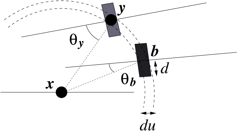
Figure 1: A schematic diagram showing absorbers at $\mathbf{x}$ and $\mathbf{y}$. The solid lines represent lines of sight, and the dashed lines the shell centered at $\mathbf{x}$, with radius $|\mathbf{y}-\mathbf{x}|$ and thickness $du$. Each of the shaded rectangles represents cylinders in three-dimensional space and shows where an absorber center must lie in order to be detected at that particular location on a line of sight.

The two shaded rectangles on this shell represent cylinders in three-dimensional space. If the center of the absorber $\mathbf{y}$ lies in a cylinder, it will be observed on the line of sight that passes through the center of that cylinder. When the absorber at $\mathbf{x}$ is at the center, the contribution of the absorber at $\mathbf{y}$ to the estimate of $K$ needs to be corrected for boundary effects, i.e. for the points in the shell $\delta B_{du}(\mathbf{x},|\mathbf{y}-\mathbf{x}|)$ not probed by the lines of sight so that an absorber could be present there but not observable. Using Ripley’s method of edge correction, the weight is the reciprocal of the probability of detecting an absorber, given that the absorber is present in the shell. This weight is approximated by the ratio of the volume of the shell $\delta B_{du}(\mathbf{x},|\mathbf{y}-\mathbf{x}|)$ to the volume of the cylinders. Specifically, the weight is given by

$$w_{\mathbf{x}}(|\mathbf{y}-\mathbf{x}|) = \frac{4\pi|\mathbf{y}-\mathbf{x}|^{2}du}{\pi d^{2}(du)\sum_{\mathbf{p}\in I_{\mathbf{x},\mathbf{y}}}(1/\cos\theta_{\mathbf{p}})}=\frac{4\pi|\mathbf{y}-\mathbf{x}|^{2}}{\pi d^{2}\sum_{\mathbf{p}\in I_{\mathbf{x},\mathbf{y}}}(1/\cos\theta_{\mathbf{p}})},$$ (1)

where $I_{\mathbf{x},\mathbf{y}}$ is the set of points in $\delta B_{0}(\mathbf{x},|\mathbf{y}-\mathbf{x}|)\cap L$, and $\theta_{\mathbf{p}}$ is the angle subtended by the line of sight that point $\mathbf{p}$ lies on, and the line joining point $\mathbf{p}$ and absorber $\mathbf{x}$. In Figure 1, $I_{\mathbf{x},\mathbf{y}}$ just consists of the points $\mathbf{y}$ and $\mathbf{b}$. The angles $\theta_{\mathbf{y}}$ and $\theta_{\mathbf{b}}$ are also indicated in Figure 1. The variable $d$ is the radius of an absorber in comoving units, and we assume it to be unknown, but fixed. The value of $d$ does not need to be specified because it gets cancelled away and does not appear in the estimator for $K$. For more details, see Section 3 where this cancellation also occurs for the estimator of the third-order statistic $\mathcal{K}$.

With weights specified by (1), Loh et al. (2001) show that estimates for $\lambda^{2}K$ are unbiased.

3 Estimating third-order statistics for the absorber catalog

It is well-known that second-order statistics do not completely describe the clustering properties of point processes. For example, Baddeley & Silverman (1984) provide an example of a non-Poisson process with the $K$ function identical to that of a homogeneous Poisson process. Third- and higher-order statistics will allow a more detailed study of clustering than just second-order statistics.

Peebles & Groth (1975) defined a three-point correlation function $\zeta$ and applied it to the Zwicky catalog. With three volume elements $dV_{1},dV_{2}$ and $dV_{3}$ that define a triangle with lengths $r_{12},r_{23}$ and $r_{13}$, Peebles & Groth (1975) wrote the probability of finding an object in each of these elements as

$$dP = \lambda^{3}[1+\xi(r_{12})+\xi(r_{23})+\xi(r_{13})+\zeta(r_{12},r_{23},r_{12})]dV_{1}dV_{2}dV_{3},$$ (2)

where $\lambda$ is the intensity or number density of the point process. Subsequent studies using the three-point correlation function frequently used a different description of the configuration of triplets, employing two distance measures and one angle measure: $s=r_{12},q=r_{23}/r_{12}$ and $\theta$, the angle between $r_{12}$ and $r_{23}$. See, for example, Gaztañaga et al. (2005); Nichol et al. (2006); Kulkarni et al. (2007). Note that in the above notation the angle is subtended at the second point. We will use the parametrization of two distances and an angle in this work.

For the study of galaxy surveys, a related quantity $Q$, called the reduced three-point correlation function is often used, where

$$\zeta(s,q,\theta)=Q(s,q,\theta)\times[\xi(r_{12})\xi(r_{23})+\xi(r_{23})\xi(r_{13})+\xi(r_{13})\xi(r_{12})].$$ (3)

The hierarchical form of (3) was proposed in Peebles & Groth (1975) based on their analyses of the Lick and Zwicky catalogs. It is an empirical form without theoretical support (Jing & Börner, 1998), but has been found to hold in other studies e.g. Szapudi et al. (2001). In analyses of the 2dFGRS and SDSS galaxy surveys, there appears to be variation of $Q$ with $\theta$ (e.g. Gaztañaga et al., 2005; Nichol et al., 2006).

In the statistics literature, the quantity $dP$ in (2) above is more commonly expressed in terms of a function $g^{(3)}$:

$$dP = \lambda^{3}g^{(3)}(r_{12},r_{23},\theta)dV_{1}dV_{2}dV_{3},$$ (4)

where we have used two distances and an angle for the parameters of $g^{(3)}$. Møller et al. (1998) refer to $\lambda^{3}g^{(3)}$ as the third-product density. Møller et al. (1998) also designed a third-order statistic to distinguish between certain classes of point process models, while Hanisch (1983) used a third-order statistic to examine inner linearities in point patterns. See also Schladitz & Baddeley (2000). These third-order statistics are integrated versions of the third-product density, and can be considered third-order versions of the second-order $K$ function. For our purposes, we define such a third-order function, which we denote by $\mathcal{K}$:

$$\mathcal{K}((0,R_{1}],(R_{2},R_{3}],\Omega) = \int_{0}^{R_{1}}\!\int_{R_{2}}^{R_{3}}\!\int_{\Omega}4\pi r_{12}^{2}r_{23}^{2}g^{(3)}(r_{12},r_{23},\theta)(2\pi\sin\theta)d\theta dr_{23}dr_{12},$$ (5)

where $(a,b]$ denotes an interval that includes $b$ but not $a$ and $\Omega=[\alpha_{1},\alpha_{2}],0\leq\alpha_{1}<\alpha_{2}\leq\pi$ is a range of angles. The third-order statistic of Møller et al. (1998) corresponds to $\mathcal{K}$ with $R_{2}=0,R_{3}=R_{1}$ and $\Omega=[0,\pi]$. The quantity $\mathcal{K}((0,R_{1}],(R_{2},R_{3}],\Omega)$ has an intuitive interpretation: given a randomly chosen object at $\mathbf{x}$, $\lambda^{2}\mathcal{K}((0,R_{1}],(R_{2},R_{3}],\Omega)$ is the expected number of object pairs at $\mathbf{y}$ and $\mathbf{z}$ such that $|\mathbf{y}-\mathbf{x}|\in(0,R_{1}],|\mathbf{z}-\mathbf{x}|\in(R_{2},R_{3}]$ and the angle subtended by $\mathbf{y}$ and $\mathbf{z}$ at $\mathbf{x}$, $\angle\mathbf{yxz}$, is in $\Omega$. To relate to the notation in (5), note that $r_{12}=|\mathbf{y}-\mathbf{x}|$ and $r_{23}=|\mathbf{z}-\mathbf{x}|$, so that $\mathbf{x}$ is point 2, at which the angle is subtended. Of particular interest is the case when $\theta$ is close to 0 or $\pi$, since this describes the property of finding triplets of points that lie close to a line. We will also be interested in the variation of $\mathcal{K}$ with $\Omega$.

Both the three-point and reduced three-point correlation functions can be obtained from $\mathcal{K}$. Consider $\mathcal{K}((0,R_{1}],(0,R_{3}],\Omega)$ where $\Omega$ is a small angle range, $(\theta-\delta\theta/2,\theta+\delta\theta/2)$, say. Then from (5) we have,

$$\frac{d^{2}\mathcal{K}}{dR_{1}dR_{3}} = 4\pi S(\Omega)R_{1}^{2}R_{3}^{2}g^{(3)}(R_{1},R_{3},\theta),$$ (6)

where $S(\Omega)$ is the solid angle formed by the part of the unit sphere that subtends an angle $\theta\in\Omega$ to the $x$-axis. Using (2), (3) and (4), $\zeta$ and thus $Q$ can be expressed in terms of $g^{(3)}$. Therefore estimates for one quantity can be converted to estimates for the other quantities.

There are different advantages to estimating $\mathcal{K}$ versus $\zeta$. Since $\mathcal{K}$ is an integral quantity, it is often smoother and thus its estimates might have better theoretical properties. It also separates the choice of bin size from the edge correction weights, so if a study of the effect of bin size or of different edge correction methods is desired, it may be more appropriate to use $\mathcal{K}$ (Stein et al., 2000). On the other hand, the hierarchical form of (3) is more simply expressed using $\zeta$ and $Q$. Having estimates of $\mathcal{K},\zeta$ and $Q$ allows for more flexibility in studying the clustering present in a dataset, so rather than advocating for one statistic over another, we recommend using all these statistics as tools for a detailed analysis.

When studying clustering of a point pattern observed in a finite region, it is important to account for the boundary of the observation region. If a point falls near a boundary, we do not get to observe all its neighboring points. This is a particularly important issue for an absorber catalog, since only a small portion of the three-dimensional space is probed by the lines of sight. In order to obtain unbiased estimates, point pairs that are observed have to be reweighted to account for the boundary effect. There are various methods to do the edge correction. These can be numerical such as in the estimators of the two-point correlation function introduced by Davis & Peebles (1983) and Hamilton (1993), or analytical such as those introduced by Ripley (1988) and Ohser (1983) for the $K$ function. See Kerscher et al. (2000) for a good review in the astronomy context.

Loh et al. (2001) found correction weights, based on the same correction procedure suggested by Ripley (1988), for estimating the $K$ function for the Vanden Berk et al. (1996) C iv absorber catalog. Loh et al. (2003) found expressions of the correction weights based on Ohser’s and Stoyan’s correction methods (Ohser & Stoyan, 1981; Ohser, 1983). Here, we obtain edge correction weights for estimating the third-order moment function $\mathcal{K}$ using Ripley’s method.

Note that since estimating a third-order statistic involves counting triplets of points, the more common analysis approach of treating the absorbers as a one-dimensional process on the lines of sight cannot be used. The absorbers have to be treated as a three-dimensional process, and the edge effects caused by the large regions of unobserved space have to be accounted for.

For fixed values of $R_{1},R_{2},R_{3},\alpha_{1}$ and $\alpha_{2}$, we estimate $\mathcal{K}$ by first estimating $\lambda^{3}A\mathcal{K}$ with

$$\sum_{\mathbf{x}\neq\mathbf{y}\neq\mathbf{z}\atop\mathbf{x},\mathbf{y},\mathbf{z}\in L}1_{(0,R_{1}]}(|\mathbf{y}-\mathbf{x}|)1_{(R_{2},R_{3}]}(|\mathbf{z}-\mathbf{x}|)1_{\Omega}(\angle\mathbf{yxz})\omega_{\mathbf{x}}(|\mathbf{y}-\mathbf{x}|,|\mathbf{z}-\mathbf{x}|,\Omega)V(|\mathbf{y}-\mathbf{x}|,|\mathbf{z}-\mathbf{x}|,\Omega),$$ (7)

and then dividing the estimate $\widehat{\lambda^{3}A\mathcal{K}}$ by an estimator of $\lambda^{3}A$. Here, $L$ is the set of lines of sight, $A=\pi d^{2}|L|$ is the volume probed by the lines of sight, $d$ is the constant radius of an absorber in comoving units, $\angle\mathbf{yxz}$ is the angle subtended by $\mathbf{y}$ and $\mathbf{z}$ at $\mathbf{x}$, and for any set $S$, $1_{S}(u)$ is an indicator function, equal to 1 if $u\in S$ and $0$ otherwise.

We find that with

$$\omega_{\mathbf{x}}(|\mathbf{y}-\mathbf{x}|,|\mathbf{z}-\mathbf{x}|,\Omega) = \frac{4\pi S(\Omega)|\mathbf{y}-\mathbf{x}|^{2}|\mathbf{z}-\mathbf{x}|^{2}(du)^{2}}{(\pi d^{2})^{2}(du)^{2}\sum_{\mathbf{p}\in I_{\mathbf{x},\mathbf{y}}}\sum_{\mathbf{q}\in I_{\mathbf{x},\mathbf{z}}}1_{\Omega}(\angle\mathbf{pxq})/(\cos\theta_{\mathbf{p}}\cos\theta_{\mathbf{q}})}$$ (8)

$$= \frac{4\pi S(\Omega)|\mathbf{y}-\mathbf{x}|^{2}|\mathbf{z}-\mathbf{x}|^{2}}{(\pi d^{2})^{2}\ \sum_{\mathbf{p}\in I_{\mathbf{x},\mathbf{y}}}\sum_{\mathbf{q}\in I_{\mathbf{x},\mathbf{z}}}1_{\Omega}(\angle\mathbf{pxq})/(\cos\theta_{\mathbf{p}}\cos\theta_{\mathbf{q}})},$$

$$V(|\mathbf{y}-\mathbf{x}|,|\mathbf{z}-\mathbf{x}|,\Omega) = \frac{A}{\pi d^{2}|L(|\mathbf{y}-\mathbf{x}|,|\mathbf{z}-\mathbf{x}|,\Omega)|}=\frac{|L|}{|L(|\mathbf{y}-\mathbf{x}|,|\mathbf{z}-\mathbf{x}|,\Omega)|},$$ (9)

the estimator in (7) is unbiased for $\lambda^{3}A\mathcal{K}$. The quantity $w_{\mathbf{x}}(|\mathbf{y}-\mathbf{x}|,|\mathbf{z}-\mathbf{x}|,\Omega)$ is the correction weight needed to account for the edge effects. It is also called the local weight in Kerscher et al. (2000). The quantity $V(|\mathbf{y}-\mathbf{x}|,|\mathbf{z}-\mathbf{x}|,\Omega)$ is sometimes referred to as Ohser’s factor (Ohser, 1983), and makes the estimator valid for longer distances. It is called a global weight in Kerscher et al. (2000). For the rest of this section, we explain how the expressions in (8) and (9) are obtained.

The denominator in the right-hand side of (8) is related to the weights found in Loh et al. (2001), specifically, to the denominator in the right-hand side of (1). In (1), the denominator is the sum of the volumes of the cylinders associated with the intersection of $\delta B_{du}(\mathbf{x},|\mathbf{y}-\mathbf{x}|)$ with the set of lines of sight $L$, less a factor of $du$. These cylinders are shown in Figure 1 and are shown again in the lower left portion of Figure 2.

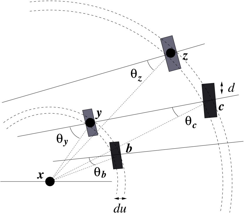
Figure 2: A schematic diagram similar to Figure 1, with an additional absorber at $\mathbf{z}$, and a shell centered at $\mathbf{x}$, with radius $|\mathbf{z}-\mathbf{x}|$ and thickness $du$. The triplet of absorbers $\mathbf{y},\mathbf{x},\mathbf{z}$ is of the desired configuration. The triplet of points $\mathbf{b},\mathbf{x},\mathbf{c}$ corresponds to a set of locations in $L$ where a triplet of absorbers of the desired configuration could potentially have been observed.

For (8), we need to consider the intersections of $\delta B_{du}(\mathbf{x},|\mathbf{z}-\mathbf{x}|)$ with $L$ as well, represented by the outer shell in Figure 2. Like in (1), $I_{\mathbf{x},\mathbf{y}}=\delta B_{0}(\mathbf{x},|\mathbf{y}-\mathbf{x}|)\cap L$ where $\delta B_{0}(\mathbf{x},|\mathbf{y}-\mathbf{x}|)$ is the sphere centered at $\mathbf{x}$ with radius $|\mathbf{y}-\mathbf{x}|$. The definition for $I_{\mathbf{x},\mathbf{z}}$ is similar. With respect to Figure 2, $I_{\mathbf{x},\mathbf{y}}$ contains the locations $\mathbf{b}$ and $\mathbf{y}$, while $I_{\mathbf{x},\mathbf{z}}$ contains the locations $\mathbf{c}$ and $\mathbf{z}$.

To get the denominator on the right-hand side of (8), we consider pairs of cylinders, one on the outer shell and one on the inner shell, i.e. a cylinder associated with a point $\mathbf{q}$ in $I_{\mathbf{x},\mathbf{z}}$ and another associated with a point $\mathbf{p}$ in $I_{\mathbf{x},\mathbf{y}}$. Each product of the volumes of these pairs of cylinders, equal to $\pi d^{2}(du)/\cos\theta_{\mathbf{p}}\times\pi d^{2}(du)/\cos\theta_{\mathbf{q}}$, is included in the sum only if the angle subtended at $\mathbf{x}$ by the centers of the cylinder pair is in the range specified by $\Omega$, i.e. if $1_{\Omega}(\mathbf{\angle pxq})=1$. In Figure 2, these pairs are highlighted by rectangles that are similarly shaded. Note that the $(du)^{2}$ term cancels because there is a corresponding term in the numerator of (8). It is also worth noting that the numerator of (8) has a form similar to the right-hand side of (6).

There may be locations in $L$ that cannot be a possible location for the absorber $\mathbf{x}$ of a triplet $\mathbf{y},\mathbf{x},\mathbf{z}$ of the desired configuration. Which locations these are depend on the actual positions and lengths of the lines of sight in $L$. The quantity $V$ in (9) accounts for this. Each location $\mathbf{a}\in L$ is in the set $L(|\mathbf{y}-\mathbf{x}|,|\mathbf{z}-\mathbf{x}|,\Omega)$ if there are points $\mathbf{b},\mathbf{c}\in L$ such that $|\mathbf{b}-\mathbf{a}|=|\mathbf{y}-\mathbf{x}|$, $|\mathbf{c}-\mathbf{a}|=|\mathbf{z}-\mathbf{x}|$ and the angle subtended by $\mathbf{b}$ and $\mathbf{c}$ at $\mathbf{a}$, $\angle\mathbf{bac}$, is in $\Omega$, i.e. $L(|\mathbf{y}-\mathbf{x}|,|\mathbf{z}-\mathbf{x}|,\Omega)$ is just the set $\{\mathbf{a}\in L:\exists\mathbf{b},\mathbf{c}\in L\mbox{ with }|\mathbf{b}-\mathbf{a}|=|\mathbf{y}-\mathbf{x}|,|\mathbf{c}-\mathbf{a}|=|\mathbf{z}-\mathbf{x}|,\angle\mathbf{bac}\in\Omega\}$. So, by definition, $\mathbf{x}$ of Figure 2 has to be in $L(|\mathbf{y}-\mathbf{x}|,|\mathbf{z}-\mathbf{x}|,\Omega)$.

To get an estimate of $\mathcal{K}$, we divide the estimator (7) by an estimate of $\lambda^{3}A$, e.g. $(N^{3}/A^{3})A=N^{3}/(\pi d^{2})^{2}|L|^{2}$. Thus, although the expression for $\omega_{\mathbf{x}}$ includes a $(\pi d^{2})^{2}$ term, the value of $d$ need not be specified when estimating $\mathcal{K}$ since it gets cancelled away by the same term in the estimate of $\lambda^{3}A$.

The proof of unbiasedness is provided in the Appendix. Note that it is the estimator of $\lambda^{3}A\mathcal{K}$ that is unbiased. The estimate $\hat{\mathcal{K}}$ that is obtained by dividing by an estimate of $\lambda^{3}A$ may be slightly biased. Such a property is called ratio-unbiasedness, and is a feature of estimators of the second-order $K$ function as well.

4 Simulation Study

We ran a simulation study to explore the performance of the estimator given in (7), with weights given in (8) and (9). Note that distances referred to here are comoving distances. We first generated a set of 1000 lines of sight in a region similar to that to be probed by the QSO lines of sight of the SDSS Catalog: a cone with half-angle of $45^{\circ}$ with Earth at its tip, bounded by comoving distance $2000<r<3300h^{-1}$ Mpc from Earth. This range of distances corresponds to the comoving distances probed by QSO lines of sight for Mg ii and C iv absorbers under the Einstein-de Sitter cosmology. A thousand realizations of a Poisson point process are then simulated on to these lines of sight, with density equal to that found in the Vanden Berk et al. (1996) catalog, 0.004 per $h^{-1}$ Mpc. We chose Poisson processes since the theoretical value of $\mathcal{K}$ is known for the Poisson model: $P=\mathcal{K}_{\mbox{\small Poi}}((0,R_{1}],(R_{2},R_{3}],\Omega)=4\pi S(\Omega)(R_{3}^{3}-R_{2}^{3})R_{1}^{3}/9$. For each realization, we estimate the third-order function $\mathcal{K}$. We then find the mean and variance of these estimates, and compare it with the theoretical Poisson value $P$. The results are shown in Figures 3 and 4.

Figure 3 shows the ratio of the mean estimates of $\mathcal{K}((0,50],(250,r],\Omega)$ to the expected Poisson value, for $\Omega=(0^{\circ},5^{\circ})$ (top left), $\Omega=(40^{\circ},50^{\circ})$ (top right), $\Omega=(55^{\circ},60^{\circ})$ (bottom left) and $\Omega=(80^{\circ},90^{\circ})$ (bottom right), plotted as a function of $r$, for $250<r\leq 330$ $h^{-1}$ Mpc (solid lines). The dashed lines show the pointwise error, equal to two times the standard deviation of the 1000 estimates. Notice that in each case, the true value of 1 lies within this band. Furthermore the mean estimated value is very close to 1 for the smaller angle ranges, with a slight bias appearing with angles close to $90^{\circ}$. We believe this is because the edge correction approximation becomes less accurate at angles close to $90^{\circ}$.

Figure 4 shows plots of the same ratio as a function of $\theta$, the midpoint of $\Omega$, from $0^{\circ}$ to $90^{\circ}$, for values of $r$ fixed at 260, 280, 300 and 320 $h^{-1}$ Mpc. The angular bin size used is $10^{\circ}$. Again, we find that the pointwise confidence band contains the true value 1, with the mean value also close to 1. These plots show the bias appearing as the angle is increased to $90^{\circ}$, with this bias becoming slightly less as the range $(250,r]$ increases.

Figure 3: Plots of the mean, over 1000 simulated realizations, of the ratio of $\hat{\mathcal{K}}((0,50],(250,r],\Omega)$ to the expected Poisson value as a function of $r$ from 250 to 330 $h^{-1}$ Mpc. The $\Omega$ for each plot is specified at the top of plot. The dashed lines refer to pointwise errors that are twice the standard deviation obtained from the simulations.

Figure 4: Plots of the mean, over 1000 simulated realizations, of the ratio of $\hat{\mathcal{K}}((0,50],(250,r],\theta)$ to the expected Poisson value as a function of $\theta$ from 0 to $90^{\circ}$, using angular bins of $10^{\circ}$. The value of $r$ for each plot is specified at the top of plot. The dashed lines refer to pointwise errors that are twice the standard deviation obtained from the simulations.

We chose the distance 50 $h^{-1}$ Mpc for $R_{1}$ since it corresponds roughly to the scale of superclustering that has been detected (Quashnock et al., 1996). With the values of $r_{23}\in(250,330]$ that we used, the ratio $r_{23}/r_{12}$ is then about 5 or 6, close to the values considered in e.g. Kulkarni et al. (2007), although the values of $r_{12}$ considered there are much smaller. We also considered values of 10 to 40 $h^{-1}$ Mpc for $R_{1}$. The results are qualitatively similar to the results for $R_{1}=50h^{-1}$ Mpc, except with slightly larger standard errors.

We also performed a simulation study using 10,000 lines of sight in the same region. The corresponding plots are similar to those of Figures 3 and 4, but with standard errors smaller by a factor of about 10 to 15, i.e. roughly of the order of the increase in the number of lines of sight. For $\Omega=(0^{\circ},5^{\circ})$, standard errors dropped only by about a factor of 5, however. This approximate relation between standard errors and the number of lines of sight is similar to that found by Loh et al. (2001).

5 Discussion and Conclusion

Measures of the third-order clustering of galaxy surveys and the cosmic microwave background are useful for the additional information they provide over measures of second-order clustering. In particular, the filamentary structure that has been found in galaxy data is more readily described by third- and higher-order measures of clustering. Recently, due to the availability of larger datasets and advances in computing, such study of higher-order clustering has been the subject of active research.

It will be desirable to study the third-order clustering of absorption systems. Absorbers are often detected at extreme comoving distances from the Earth. Since absorbers are believed to be due to gas clouds near galaxies, an analysis of the third-order clustering of absorbers can serve as a complementary analysis to that of large galaxy surveys, enabling comparison of the local filamentary structure to that of the early universe. Studying the third-order structure of absorbers might also provide greater understanding of their nature. Finally, absorption systems consist of non-luminous matter. Understanding the clustering of absorbers can yield insight into the link between luminous and non-luminous matter in the universe.

In this paper, we define a third-order moment function $\mathcal{K}$ that is an integrated version of the three-point correlation function, much like the relation between the second-order Ripley’s $K$ function and the two-point correlation function. We provide expressions for the weights necessary to correct for the boundary effects so that this function can be estimated for an absorber catalog. Our simulation study shows that the estimator gives correct results (i.e. including correctly accounting for the boundary effects), at least for the theoretically simple Poisson process.

Studies on large-scale structure with galaxy surveys have shown the existence of structures of the order of 100 $h^{-1}$ Mpc in size (Kirshner et al., 1981; Geller & Huchra, 1989; da Costa et al., 1994). In analyses of second-order clustering of the Las Campanas and SDSS surveys, Landy et al. (1996) and Eisenstein et al. (2005) respectively found peaks on scales of around 100 $h^{-1}$ Mpc. Quashnock et al. (1996) also found evidence of superclustering on these scales in their analysis of C iv absorption systems. Loh et al. (2001) also found evidence of clustering up to 100 $h^{-1}$ Mpc and possibly beyond. Studies on galaxy clustering have focused on smaller scales. Gaztañaga et al. (2005); Nichol et al. (2006) and Kulkarni et al. (2007) followed the example of Jing & Börner (1998), using $r_{12}$ from 1 to 10 $h^{-1}$ Mpc and $r_{23}/r_{12}$ between 1 and 4, and studied the variation in the reduced three-point correlation function $Q$ with angle.

The choice of $R_{1},R_{2},R_{3}$ and $\Omega$ for $\mathcal{K}$ would thus depend on the aim of the analysis. For comparisons with the findings of e.g. Jing & Börner (1998), the focus will be to study the variation of $\mathcal{K}$ with $\Omega$, with the distance measures close to the values used there. For studies on superclustering and large-scale structure, comoving distances of 100 $h^{-1}$ Mpc and beyond for one or both of $r_{12}$ and $r_{23}$ will be of interest. An initial study will probably use $\Omega=[0,\pi]$, studying clustering at various distances, followed by more detailed analyses with smaller angular ranges.

We are not aware of any other work on estimating third-order clustering specifically for absorber catalogs. Unfortunately, we do not have a large enough catalog of absorbers to obtain meaningful estimates of the third-order function. With the much larger absorber catalog that is being collected by the Sloan Digital Sky Survey, a detailed study of the third-order clustering of absorbers will become feasible. From our simulation studies, we found that the standard errors of estimates of $\mathcal{K}$ for an absorber catalog scale roughly on the order of the reciprocal of the number of lines of sight. This agrees with the findings of Loh et al. (2001) for standard errors of estimates of the $K$ function for absorber catalogs. Thus we expect that with the SDSS absorber catalog with approximately 50,000 lines of sight, the standard errors of the estimates of $\mathcal{K}$ will be roughly a factor of 50 smaller than the standard errors found in our simulation study with 1000 lines of sight. The actual increase in precision for a particular absorber catalog will of course depend on factors such as the actual spatial locations of the lines of sight and the density of the observed absorbers.

Appendix A Appendix

Here, we prove that the estimator (7) with weights $\omega_{\mathbf{x}}$ and $V$ given by (8) and (9) is unbiased. Let $L$ represent the lines of sight, $\delta B_{\Delta}(\mathbf{x},h)$ denote a shell with center $\mathbf{x}$, radius $h$ and thickness $\Delta$. We write $(h,\gamma)$ for the polar coordinates of vector $\mathbf{h}$, $|\cdot|$ for Euclidean distance, area or volume depending on the context, $A=\pi d^{2}|L|$ for the volume probed by the lines of sight and $1_{L}(\mathbf{x})$ for the indicator function, with $1_{L}(\mathbf{x})=1$ if $\mathbf{x}\in L$ and 0 otherwise.

Write $f(\mathbf{x},\mathbf{y},\mathbf{z})=1_{L}(\mathbf{x})1_{L}(\mathbf{y})1_{L}(\mathbf{z})1_{(0,R_{1}]}(|\mathbf{y}-\mathbf{x}|)1_{(R_{2},R_{3}]}(|\mathbf{z}-\mathbf{x}|)1_{\Omega}(\angle\mathbf{yxz})\omega_{\mathbf{x}}(|\mathbf{y}-\mathbf{x}|,|\mathbf{z}-\mathbf{x}|,\Omega)V(|\mathbf{y}-\mathbf{x}|,|\mathbf{z}-\mathbf{x}|,\Omega))$, where $\Omega=[\alpha_{1},\alpha_{2}]$ represents the range of angles between $\alpha_{1}$ and $\alpha_{2}$. Then the estimator in (7) is $\sum_{\mathbf{x}\neq\mathbf{y}\neq\mathbf{z}}f(\mathbf{x},\mathbf{y},\mathbf{z})$, with

$$E\left(\sum_{\mathbf{x}\neq\mathbf{y}\neq\mathbf{z}}f(x,y,z)\right) = \lambda^{3}\int\!\!\!\int\!\!\!\int f(\mathbf{x},\mathbf{x}+\mathbf{h},\mathbf{x}+\mathbf{k})g^{(3)}(\mathbf{x},\mathbf{x}+\mathbf{h},\mathbf{x}+\mathbf{k})\,d\mathbf{h}\,d\mathbf{k}\,d\mathbf{x}$$

$$= \lambda^{3}\int_{\mathbb{R}^{3}}\int_{0}^{R_{1}}\!\!\!\int_{R_{2}}^{R_{3}}\!\!\!\int_{\delta B_{0}(\mathbf{0},k)}\int_{\delta B_{0}(\mathbf{0},h)}1_{L}(\mathbf{x})1_{L}(\mathbf{x}+(h,\gamma))1_{L}(\mathbf{x}+(k,\beta))$$

$${}\times 1_{\Omega}(\gamma-\beta)\omega_{\mathbf{x}}(h,k,\Omega)V(h,k,\Omega)h^{2}k^{2}g^{(3)}((h,\gamma),(k,\beta))\,d\gamma\,d\beta\,dh\,dk\,d\mathbf{x}.$$

In the first equality above, we have expressed $g^{(3)}$ in terms of three vector quantities $\mathbf{x},\mathbf{x}+\mathbf{h}$ and $\mathbf{x}+\mathbf{k}$. If stationarity is assumed, the specification of $\mathbf{x}$ in $g^{(3)}$ is redundant. Thus we have removed the dependence on $\mathbf{x}$ in $g^{(3)}$ in the next line. We have also expressed $\mathbf{h}$ and $\mathbf{k}$ in polar coordinates. Now, with the further assumption of isotropy, $g^{(3)}(\mathbf{h},\mathbf{k})$ depends only on the direction of $\mathbf{h}$ relative to $\mathbf{k}$ (or vice versa). This simplifies the expression above, so that

$$E\left(\sum_{\mathbf{x}\neq\mathbf{y}\neq\mathbf{z}}f(\mathbf{x},\mathbf{y},\mathbf{z})\right) = \lambda^{3}\int_{\mathbb{R}^{3}}\int_{0}^{R_{1}}\!\!\!\int_{R_{2}}^{R_{3}}\!\!\!V(h,k,\Omega)1_{L}(\mathbf{x})\omega_{\mathbf{x}}(h,k,\Omega)$$

$${}\times\int_{\delta B_{0}(\mathbf{0},k)}1_{L}(\mathbf{x}+(k,\beta))k^{2}$$

$${}\quad\times\left[\int_{\delta B_{0}(\mathbf{0},h)}1_{\Omega}(\alpha)1_{L}(\mathbf{x}+(h,\beta+\alpha))h^{2}g^{(3)}(h,k,\alpha)\,d\alpha\right]\,d\beta\,dh\,dk\,d\mathbf{x},$$

where $\alpha$ denotes the angle on the sphere relative to $(k,\beta)$. Under the assumption that $g^{(3)}$ is slowly varying over $\Omega$, the expression in the square bracket above is equal to

$$1_{L(h,\beta+\Omega)}(\mathbf{x})g^{(3)}(h,k,\Omega)\sum_{\mathbf{p}\in\delta B_{0}(\mathbf{x},h)\cap L}1_{\Omega}(\angle\mathbf{px}(\mathbf{x}+\mathbf{k}))\frac{\pi d^{2}}{\cos\theta_{\mathbf{p}}},$$

so that

$$E\left(\sum_{\mathbf{x}\neq\mathbf{y}\neq\mathbf{z}}f(\mathbf{x},\mathbf{y},\mathbf{z})\right) = \lambda^{3}A\int_{\mathbb{R}^{3}}\int_{0}^{R_{1}}\!\!\!\int_{R_{2}}^{R_{3}}\!\!\!\frac{1_{L}(\mathbf{x})}{\pi d^{2}|L(h,k,\Omega)|}\omega_{\mathbf{x}}(h,k,\Omega)g^{(3)}(h,k,\Omega)$$

$${}\times\left[\int_{\delta B_{0}(\mathbf{0},k)}1_{L(h,\beta+\Omega)}(\mathbf{x})1_{L}(\mathbf{x}+(k,\beta))\right.$$

$${}\quad\times\left.\left\{\sum_{\mathbf{p}\in\delta B_{0}(\mathbf{x},h)\cap L}1_{\Omega}(\angle\mathbf{px}(\mathbf{x}+\mathbf{k}))\frac{\pi d^{2}}{\cos\theta_{\mathbf{p}}}\right\}k^{2}\,d\beta\right]\,dh\,dk\,d\mathbf{x}$$

$$= \lambda^{3}A\int_{\mathbb{R}^{3}}\int_{0}^{R_{1}}\!\!\!\int_{R_{2}}^{R_{3}}\!\!\!\frac{\omega_{\mathbf{x}}(h,k,\Omega)}{\pi d^{2}|L(h,k,\Omega)|}1_{L(h,k,\Omega)}(\mathbf{x})g^{(3)}(h,k,\Omega)$$

$${}\times\left(\sum_{\mathbf{p}\in\delta B_{0}(\mathbf{x},h)\cap L}\sum_{\mathbf{q}\in\delta B_{0}(\mathbf{x},k)\cap L}1_{\Omega}(\angle\mathbf{pxq})\frac{\pi d^{2}}{\cos\theta_{\mathbf{p}}}\frac{\pi d^{2}}{\cos\theta_{\mathbf{q}}}\right)\,dh\,dk\,d\mathbf{x}.$$

The above expression in the round brackets is the denominator of $\omega_{\mathbf{x}}(h,k,\Omega)$. Further simplification yields

$$E\left(\sum_{\mathbf{x}\neq\mathbf{y}\neq\mathbf{z}}f(\mathbf{x},\mathbf{y},\mathbf{z})\right) = \lambda^{3}A\int_{\mathbb{R}^{3}}\int_{0}^{R_{1}}\!\!\!\int_{R_{2}}^{R_{3}}\!\!\!\frac{1_{L(h,k,\Omega)}(\mathbf{x})}{\pi d^{2}|L(h,k,\Omega)|}4\pi h^{2}k^{2}S(\Omega)g^{(3)}(h,k,\Omega)\,dh\,dk\,d\mathbf{x}$$

$$= \lambda^{3}A\int_{0}^{R_{1}}\!\!\!\int_{R_{2}}^{R_{3}}\!\!\!4\pi h^{2}k^{2}S(\Omega)g^{(3)}(h,k,\Omega)\,dh\,dk$$

$$= \lambda^{3}A\mathcal{K}((0,R_{1}],(R_{2},R_{3}],\Omega).$$

References

- Baddeley & Silverman (1984) Baddeley, A. J., & Silverman, B. W. 1984, Biometrics, 40, 1089
- Crotts (1985) Crotts, A. P. S. 1985, ApJ, 298, 732
- Crotts et al. (1985) Crotts, A. P. S., Melott, A. L., York, D. G., & Fry, J. N. 1985, Phys. Lett. B, 155, 251
- da Costa et al. (1994) da Costa, L. N., et al. 1994, ApJ, 424, L1
- Davis & Peebles (1983) Davis, M., & Peebles, P. J. E. 1983, ApJ, 267, 465
- Dinshaw & Impey (1996) Dinshaw, N., & Impey, C. D. 1996, ApJ, 458, 73
- Eisenstein et al. (2005) Eisenstein, D. J., Zehavi, I., Hogg, D. W., & Scoccimarro, R. 2005, ApJ, 633, 560
- Fry & Peebles (1980) Fry, J. N., & Peebles, P. J. E. 1980, ApJ, 238, 785
- Gaztañaga et al. (2005) Gaztañaga, E., Norberg, P., Baugh, C. M., & Croton, D. J. 2005, MNRAS, 364, 620
- Gaztañaga & Scoccimarro (2005) Gaztañaga, E., & Scoccimarro, R. 2005, MNRAS, 361, 824
- Geller & Huchra (1989) Geller, M. J., & Huchra, J. P. 1989, Science, 246, 897
- Hamilton (1993) Hamilton, A. J. S. 1993, ApJ, 417, 19
- Hanisch (1983) Hanisch, K.-H. 1983, Math. Oper. Ser. Statist., 14, 421
- Heisler et al. (1989) Heisler, J., Hogan, C. J., & White, S. D. M. 1989, ApJ, 347, 52
- Jing & Börner (1998) Jing, Y. P., & Börner, G. 1998, ApJ, 503, 37
- Kerscher et al. (2000) Kerscher, M., Szapudi, I., & Szalay, A. S. 2000, ApJ, 535, L13
- Kirshner et al. (1981) Kirshner, R. P., Oemler, A., Schechter, P. L., & Shectman, S. A. 1981, ApJ, 248, L57
- Kulkarni et al. (2007) Kulkarni, G. V., Nichol, R. C., Sheth, R. K., Seo, H.-J., Eisenstein, D. J., & Gray, A. 2007, MNRAS, 378, 1196
- Landy et al. (1996) Landy, S. D., Schectman, S. A., Lin, H., Kirshner, R. P., Oemler, A. A., & Tucker, D. 1996, ApJ, 456, L1
- Loh et al. (2001) Loh, J. M., Quashnock, J. M., & Stein, M. L. 2001, ApJ, 560, 606
- Loh et al. (2003) Loh, J. M., Stein, M. L., & Quashnock, J. M. 2003, J. Am. Stat. Assoc., 98, 522
- Martínez et al. (1998) Martínez, V. J., Pons-Bordería, M.-J., Moyeed, R. A., & Graham, M. J. 1998, MNRAS, 298, 1212
- Martínez & Saar (2002) Martínez, V. J., & Saar, E. 2002, Statistics of the Galaxy Distribution (Boca Raton: Chapman and Hall/CRC)
- Møller et al. (1998) Møller, J., Syversveen, A. R., & Waagepetersen, R. P. 1998, Scand. J. Stat., 25, 451
- Nichol et al. (2006) Nichol, R. C., et al. 2006, MNRAS, 368, 1507
- Ohser (1983) Ohser, J. 1983, Math. Oper. Ser. Statist., 14, 63
- Ohser & Stoyan (1981) Ohser, J., & Stoyan, D. 1981, Biometric J., 23, 523
- Peebles (1980) Peebles, P. J. E. 1980, The Large-Scale Structure of the Universe (New Jersey: Princeton University Press)
- Peebles (1993) —. 1993, Principles of Physical Cosmology (New Jersey: Princeton University Press)
- Peebles & Groth (1975) Peebles, P. J. E., & Groth, E. J. 1975, ApJ, 196, 1
- Quashnock & Stein (1999) Quashnock, J. M., & Stein, M. L. 1999, ApJ, 515, 506
- Quashnock & Vanden Berk (1998) Quashnock, J. M., & Vanden Berk, D. E. 1998, ApJ, 500, 28
- Quashnock et al. (1996) Quashnock, J. M., Vanden Berk, D. E., & York, D. G. 1996, ApJ, 472, L69
- Ripley (1988) Ripley, B. D. 1988, Statistical Inference for Spatial Processes (New York: Wiley)
- Schladitz & Baddeley (2000) Schladitz, K., & Baddeley, A. J. 2000, Scand. J. Stat., 27, 657
- Sefusatti & Scoccimarro (2005) Sefusatti, E., & Scoccimarro, R. 2005, Phys. Rev. D, 71, 063001
- Stein et al. (2000) Stein, M. L., Quashnock, J. M., & Loh, J. M. 2000, Ann. Stat., 28, 1503
- Szapudi et al. (2001) Szapudi, I., Postman, M., Lauer, T., & Oegerie, W. 2001, ApJ, 548, 114
- Tripp & Bowen (2005) Tripp, T. M., & Bowen, D. V. 2005, in Probing Galaxies through Quasar Absorption Lines: Proc. IAU 199
- Tytler et al. (1993) Tytler, D., Sandoval, J., & Fan, X.-M. 1993, ApJ, 405, 57
- Vanden Berk et al. (1996) Vanden Berk, D. E., Quashnock, J. M., York, D. G., & Yanny, B. 1996, ApJ, 469, 78
- York et al. (2000) York, D. G., et al. 2000, AJ, 120, 1579