Beyond Chaos

Abstract.

The first part of this paper defines recursive interactions by means of logistic functions and derives a general result on the way interacting systems evolve in attractors. It also defines the notion of coevolution trajectory and presents a new family of attractors: orbital attractors (including single, irregular, folded, complex and discontinuous orbits). The second part summarizes the results of a first experimental analysis of recursive interactions in both binary and multiple interactions. Among other results, this analysis reveals that interacting systems may easily evolve from chaos to order.

1. Introduction

Mathematical continuity makes no sense in biology. The biosphere is radically discontinuous, i.e. discrete; it is the paradigm of discreteness. Each living being is a discrete unity, unique and unrepeatable, that emerges and self maintains at the expense of a discrete net of metabolic reactions governed by a discrete net of discrete information units. Each living being forms part of a discrete group of discrete individuals which in turns form part of a discrete net of ecological interactions. But living organisms are not the only discrete objects in the universe, matter and energy are also discrete. In consequence, all natural processes involving matter or energy interchanges have to be of a discrete nature. Even space and time could be discrete as has been repeatedly suggested from different areas of physics ([6], [7], [9], [19], [13], [10], [24], [4], [24], [2], [21], [11], [5], [3], [22], [1] , [12], [26], [23], [17], [3]). In these conditions, and being the best model of any object the very object itself, what should be put into question is not the role of discrete models [8] but the role of mathematical continuity in an essentially discontinuous world.

In addition of being discrete and interactive, living organisms are also recursive. Each generation determines the next one through a reproductive process that is not exact, giving therefore the appropriate opportunity to evolution. It is then clair the reason for which biology has always been interested in discrete and recursive models. Among them the logistic function, perhaps the most simple and productive model of some biological significance. From the pioneering works of Stanislaw Ulam, Paul Stein [25], Nicholas C. Metropolis [20] and Robert May [18] to nowadays, iterative calculus and the logistic function have been an inexhaustible source of surprising results, from deterministic chaos to periodic attractors; results that, on the other hand, were immediately generalized by the so called principle of universality. As is well known, the control parameter $\lambda$ of a logistic function:

$$x_{n+1}=4\lambda x_{n}(1-x_{n})$$ (1)

determines the system evolution, particularly the type of attractor it finally falls in. Now then, biological systems do not evolve separately but immerse in a complex interaction network. For this reason biology has also been interested in modeling interactions. Most of those models, as the classical Lotka-Volterra, are defined in terms of differential (or finite differences) equations. But as far as I know, biological interactions have never been modeled by logistic functions. As we will immediately see, biological (and non biological) interactions can easily be modeled by means of this type of functions. And the results cannot be more interesting from both the mathematical and the biological point of view. In fact, on the one hand recursive logistic interactions are a new source of new mathematical objects as coevolution trajectories or orbital attractors. On the other, they provide us a new way of examining coevolution processes and derive some significant results on the way systems coevolve. For instance, that interacting systems may coevolve from chaotic regimes to stable states defined by periodic attractors of low period; or that complex attractors, as fractal or chaotic, may suddenly evolve in single periodic attractors; or that systems to the brink of extinction may be completely recovered and stabilized thanks to its recursive interactions with other systems; or, in the case of multiple interactions, that system stability grows with the number of interactions.

The discussion that follows begins by defining the appropriate theoretical notions, from which a general result related to the way interacting systems evolve in attractors is formally derived. In the following two sections I define some new mathematical objects as the coevolution trajectory of two interacting systems and a new family of attractors. Finally, I resume the results of a first experimental work on recursive logistic interactions, including a short presentation of multiple interactions. Evidently, the field to explore is immense and what follows is but a simple introductory note. All numerical and graphical data have been obtained with the aid of InterCalculus [16], a computer application developed to analyze recursive interactions by means of logistic functions.

2. Recursive logistic interactions: Definitions

Let us consider two systems $X$ and $Y$ modeled by two logistic real functions:

$$x_{n+1}=\lambda_{x}x_{n}(1-x_{n})$$

$$y_{n+1}=\lambda_{y}y_{n}(1-y_{n})$$

An elemental way to make both functions mutually dependent consists in defining the control parameter of each function in terms of the other function variable:

$$x_{n+1}=g_{x}(y_{n})x_{n}(1-x_{n})$$

$$y_{n+1}=g_{y}(x_{n})y_{n}(1-y_{n})$$

If $g_{x}(y_{n})$, the interaction function of system $X$ with system $Y$, is decreasing the interaction of system $X$ with system $Y$ will be said negative; if it increasing the interaction will be said positive. The same applies to $g_{y}(x_{n})$, the interaction function of system $Y$ with system $X$. There are many ways to define the interaction functions $g_{x}$ and $g_{y}$. Here we will use the following:

$$g_{x}(y_{n})=4(1-S_{x}y_{n})$$

for negative interactions, and:

$$g_{x}(y_{n})=4S_{x}y_{n}$$

for positive ones. In both cases, $S_{x}$ represents the sensitivity of system $X$ to system $Y$, i.e. a measure of the effects of system $Y$ on system $X$. It will take its values within the real half closed interval $(0,1]$. Similarly, for the interaction of system $Y$ with system $X$ we will have:

$$g_{y}(x_{n})=4(1-S_{y}x_{n})$$

$$g_{y}(x_{n})=4S_{y}x_{n}$$

It is now immediate to define the following three types of recursive logistic interactions (recursive interactions from now on):

1. Negative-Negative:

   $$x_{n+1}=4(1-S_{x}y_{n})x_{n}(1-x_{n})$$ (2)

   $$y_{n+1}=4(1-S_{y}x_{n})y_{n}(1-y_{n})$$ (3)

2. Positive-Negative:

   $$x_{n+1}=4S_{x}y_{n}x_{n}(1-x_{n})$$ (4)

   $$y_{n+1}=4(1-S_{y}x_{n})y_{n}(1-y_{n})$$ (5)

3. Positive-Positive:

   $$x_{n+1}=4S_{x}y_{n}x_{n}(1-x_{n})$$ (6)

   $$y_{n+1}=4S_{y}x_{n}y_{n}(1-y_{n})$$ (7)

Here we will exclusively deal with these recursive interactions. From now on negative-negative interactions will be referred to as NN interactions; positive-negative as PN; and positive-positive as PP.

The above definitions can immediately be generalized for any number of systems. In effect, consider $m$ systems $\langle X_{i}\rangle_{i=1,2,\dots m}$ being each modeled by a logistic function of a real variable $x_{i}$. Assume that all systems interact which each other. Their evolution can be expressed as:

$$x_{i,\,n+1}=\frac{1}{m-1}\sum_{\underset{j\neq i}{j=1}}^{m}g_{x_{i}}(x_{j})x_{i,n}(1-x_{i,n})$$ (8)

where $x_{i,n}$ represent the $n$-th generation of system $x_{i}$; $g_{x_{i}}(x_{j})$ is the interaction function of system $X_{i}$ with system $X_{j}$, a function that will be given by $4S_{i,j}x_{j,n}$ if that interaction is positive, or $4(1-S_{i,j}x_{j,n})$ if it is negative, being $S_{i,j}$ the sensitivity of system $X_{i}$ to system $X_{j}$. Equations (8) can be easily computerized so that it is possible to make both numerical and graphical analysis of the evolution of any number of interacting systems.

3. Attractors theorem

We will prove now a general and basic result that states the simultaneity and equivalence of the attractors the interacting systems evolve in.

Theorem 1.

Let $X$ and $Y$ be two systems that interact with each other. A necessary and sufficient condition for system $X$ to fall in a period-k attractor is that system $Y$ also falls in a period-k attractor.

Proof.

Assume that system $X$ falls in a period-k attractor. From a certain integer $i>0$ it will hold:

$$x_{n}=x_{n+k},\ \forall n>i$$ (9)

On the other hand we will have

$$x_{n}=S(y_{n-1})x_{n-1}(1-x_{n-1})$$

$$x_{n+k}=S(y_{n+k-1})x_{n+k-1}(1-x_{n+k-1})$$

where $S(y_{n-1})$ is $4(1-S_{x}y_{n-1})$ if the interaction of $X$ with $Y$ is negative, or $4S_{x}y_{n-1}$ if it is positive. The same applies to $S(y_{n+k-1})$. According to (9) we can write:

$$S(y_{n-1})x_{n-1}(1-x_{n-1})=S(y_{n+k-1})x_{n+k-1}(1-x_{n+k-1})$$

and taking into account that $x_{n-1}=x_{n+k-1}$ we have:

$$S(y_{n-1})=S(y_{n+k-1})$$

That is to say:

$$4(1-S_{x}y_{n-1})=4(1-S_{x}y_{k+n-1})$$

if the interaction of $X$ with $Y$ is negative; or:

$$4S_{x}y_{n-1}=4S_{x}y_{k+n-1}$$

if it is positive. In both cases, we immediately get:

$$y_{n-1}=y_{n+k-1},\ \forall n>i$$

which implies that system $Y$ has also fallen in a period-k attractor. This proves that if system $X$ evolves in a period-k attractor, so evolves system $Y$. A similar argument proves the complementary result.

∎

The above theorem applies only to binary interactions. In the case of multiple interactions, in fact, systems do not reach simultaneously their final attractor; although, in most cases, once a first system falls in its final attractor the remainder ones also fall in their respective final attractors after a few number of iterations. I think attractors theorem is not the only conclusion that can be formally derived for binary interactions. Experimental research strongly suggests that, among others, the following results could also be formally proved:

• In NN interactions, the less sensitive system always goes ahead of the most sensitive one.

• In PN interactions, the system suffering the negative interaction always goes ahead of the other.

• Coevolution trajectories in NN interactions are symmetrical with respect the bisectors of $(0,1)\times(0,1)$.

4. Coevolution trajectories

Recursive interaction invariably leads to a final attractor that may be periodic, chaotic, fractal or of some new types, as we will immediately see. The set of points each interacting systems traverses towards its final attractor defines its coevolution trajectory (CT). It usually consists of two or more well defined lines, branches from now on, usually with diagonal symmetry although they can also exhibit radial or spiral symmetry. Each interacting system has its own CT, being both CT very similar.

Systems evolve along the branches of their CT by cyclically stepping from a branch to other, always in the same order, so that they exhibit a remarkable periodic behaviour. Due to the discrete nature of iterations, CT are not continues but discrete lines, although the density of points can be extremely high and we have to magnify them thousands of millions times to make discontinuity visible. Naturally, in these superdense regions the progress towards the final attractor is also extremely slow. Coevolution trajectories are then sets of points -usually lines- in the interval $[0,1]\times[0,1]$ of $\mathbb{R}^{2}$ along which interacting systems evolve towards their respective final attractors. As far as they have been examined, the coevolution trajectories of both systems are geometrically similar, with the same number of branches and the same type of symmetry. The branches of a CT may converge or diverge from the central point $(0.5,0.5)$, being the changes simultaneous in all branches of both CT.

There also exists CT trough which systems evolve from chaos to non chaotic attractor (periodic, fractal or orbital) or even from a chaotic regime to other different chaotic regime. While traversing their respective CT, one of the systems goes always ahead of the other (the less sensitive in the case of NN interactions, and the one suffering the negative interaction in PN interactions). With the appropriate initial seeds it is possible, however, to start from an inverted position. In these cases an inversion of the CT occurs thanks to which the systems recover its normal relative position. To go ahead of the other seems to be a general law that operates even in chaotic regimes.

5. Orbital attractors

As in the case of single logistic recursion, recursive interactions also end up by reaching a final attractor. Apart from the well known periodic, fractal and chaotic attractors, in the case of recursive interactions we can also observe at least a new family of attractors that we will term orbital attractors. An orbital attractor is typically composed of one or more closed lines (orbits) which are usually eccentric. Each orbit its initially a discontinuous set of segments which progressively extend in the same direction so that finally they overlap and close the line. In some cases the orbits are single lines while in other they have a complex internal structure. Systems trapped in an orbital attractor behave as if they were orbiting, although their true behaviour is a little more complex. In fact, they jump cyclically from an orbit to other always in the same order and in such a way that the successive jumps on the same orbit take place on different segments, always in the same order. All segments grow in the same direction so that after a few interactions each segment reaches the next one, although, being of a discontinuous nature, their respective points do not coincide, each segment continues indefinitely by occupying the empty gaps along the orbit. After a considerable number of iterations, each segment reaches itself and progress trough its own gaps. This way of progressing suggest the possibility that after a huge number of iterations all orbital attractors finally end in a periodic attractor.

The orbits of an orbital attractor may be at least of one of the following types:

1. Single

2. Irregular

3. Folded

4. Complex

5. Discontinuous

The lines of a single orbit do not exhibit internal structure, they always appear as single lines even if we magnify them by several billions times. The same apply to irregular and discontinuous orbits although in these cases the lines exhibit more or less irregular forms, as complex indentations. Folded orbit exhibit a complex non fractal internal structure of folded lines in the regions of maximum curvature, this structure seems disappear in the less curvature regions. This is also the case of complex orbits, although in these orbits the internal structure is extremely complex, perhaps of a fractal nature. In the case of discontinuous orbits, the segments do not extend and maintain the empty gaps between them. After a certain number of iterations these attractors degenerates in a single period attractor.

A remarkable characteristic of attractors in recursive logistic interactions is that chaotic, fractal and orbital attractors may suddenly evolve in a periodic attractor whose points presumably belong to the original attractor. It is also remarkable the existence (at least in NN interactions) of periodic attractors whose attraction decreases exponentially as systems approach them, so that it takes thousands of millions of iterations to progress one decimal cipher towards the attractor final value. They could be termed asymptotic attractors. It is possible that no finite number of iterations suffices for the system to attaint the attractor (in the same sense that the limit of a sequence cannot be reached by the successive terms of the sequence).

6. Negative-negative interactions

In accordance with the above definition (2)-(3), in NN interactions the growth of a systems is always to the detriment of the other. Thus, NN interactions model the coevolution of two systems that compete with each other. The results will depend on the sensitivities and on the initial seeds of both systems, although the sensitivity dependence is stronger. The coevolution of interacting systems is therefor controlled by four real number in the interval $(0,1]$, which means a huge number of possibilities to examine, each representing a possible coevolution history. Although only an insignificant number of cases has been examined, the following conclusions could be of general application:

1. The branches of the coevolution trajectories are symmetrical with respect to the bisector, $x_{n+1}=x_{n}$ in the case of system $X$, or $y_{n+1}=y_{n}$ in the case of system $Y$).

2. All branches of a CT are geometrically similar, with same length and the same point density.

3. Systems traverse the branches of their respective CT by stepping from one branch to other, always in the same order so that they exhibit a remarkable periodic behaviour while evolving towards the final attractor.

4. The oscillations in NN interactions are synchronic, i.e. low and high values are simultaneously reached by both systems at the same successive iterations.

5. There is a high degree of correlation between the successive values reached by both systems. The correlation coefficient is in most cases greater than 0.9, even if both systems have evolved in chaotic attractors.

6. The system of less sensitivity go always ahead of the other. That is to say, the values successively reached by the less sensitive system are always greater than those reached by the other. This result coincides with St Matthew Theorem, a formal conclusion derived from independent thermodynamical considerations (internal entropy production) [15].

7. Systems evolves in an attractor that may be periodic, chaotic, fractal, orbital or asymptotic. Low period attractors are perhaps the most frequent in NN interactions.

8. Both systems evolves always in the same type of attractor.

9. Each point of a periodic attractor has its own independent branch in the CT. Although periodic attractors can also result from the degeneration of a complex attractor (chaotic, fractal or orbital).

10. When systems fall in orbital attractors, the orbit of the less sensitive system always raises over the orbit of the more sensitive one. It is also of less size, which means that the less sensitive system is more stable.

11. Systems can evolve from a chaotic regime to a single periodic attractor.

12. Systems can evolve from order to chaos after traversing their respective regular and symmetrical CT. Or in other words, after a long stage of periodic behaviour the interacting systems can evolve to a chaotic regime.

13. Systems can evolve from an initial chaotic regime to other different final chaotic regime. Between both chaotic regimes, systems exhibit a regular periodic behaviour while traversing their respective CT.

14. Chaotic attractors extend on a broad region and exhibit a typical internal structure of parabolic gaps.

15. In certain cases, both systems have similar CT although they are traversed in opposite senses (trajectory inversions).

16. The extinction of a system (to reach the value of 0) is extremely rare.

7. Positive-negative interactions

According to (2)-(3) the effects of PN interactions are different in both interacting system: one of them benefits from the growth of the other while this other is negatively affected by the growth of the first. This type of interaction, therefore, models prey-predator interactions. As in the case of NN interactions, the coevolution of both systems also depends on four real variables within the real interval $(0,1)$: the sensitivities and the initial seeds of both systems. Consequently there is also here a huge number of possibilities to explore. The behaviour diversity is now even greater than in the NN case. Some of the most relevant characteristics of this type of recursive interaction are the following:

1. The coevolution trajectories of both systems are similar, although the length of the branches may be different.

2. The coevolution trajectories can be convergent or divergent, or may suddenly change from convergent to divergent (or viceversa). As in the NN case, they are symmetrical with respect to the bisector $x_{n+1}=x_{n}$ in the case of system $X$, or $y_{n+1}=y_{n}$ in the case of system $Y$.

3. The system suffering the positive interaction (predator system) is more affected by the interaction and may evolve to extinction. In these cases the other system (prey system) remains in a chaotic attractor.

4. It has not been observed that both systems evolves in a chaotic attractor.

5. Both systems may evolve from a chaotic regime to any other non chaotic attractor.

6. Being on the brink of extinction, the predator systems may suddenly recover and evolve to an stable non chaotic attractor.

7. For high values of sensitivities, the branches of both CT are either radial or spiral.

8. Spiral trajectories may be more or less dense, and the number of their corresponding branches is variable.

9. The center of spiral trajectories is a single period-1 attractor.

10. As in the cases of natural prey-predator interactions, systems oscillate asynchronously, so that when a system reaches a high value the other reaches a low one, and viceversa.

11. Contrarily to the NN case, trajectory inversions have not been observed.

12. Single attractors of period-1 are frequent. They may be reached through one or more (convergent) branches.

13. Some orbital attractors exhibit very complicated forms in their regions of maximum curvature (folded orbits and complex orbits).

14. Orbital attractors of the systems suffering the negative interaction always raises over the orbital attractor of the system suffering the positive interaction. They are also of less size than it.

8. Positive-positive interactions

PP interactions model pure cooperation. There are sufficient experimental reasons to conclude that in all cases both systems evolve to extinction. The only exception is the elemental case $S_{x}$ = $S_{y}$ = 1; $x_{0}$ = $y_{0}$ = 0.5, which evolve to the single attractor $0.5$. Even in the case of multiple interactions systems evolve to extinction if the number of PP interactions is sufficiently high. From thermodynamic analysis we know, on the other hand, that this type of interaction does not have asymmetrical coevolution trajectories of minimum entropy production. The only trajectory of minimum entropy in this case is the bisector $y=x$.

9. Multiple interactions

Nature is not a set of isolated couples of systems that interact with each other. It is rather composed of an immense and complex interaction network in which participate millions of systems that interact with many other different systems. It makes sense therefore to consider the possibility of analyzing more complicated situations than the simple binary cases we have just examined. As we have seen, binary logistic interactions can be easily generalized to any number of interacting systems (8). In these conditions, attractors theorem no longer holds and the theoretical study is much more complicated than in the binary case. Fortunately, we can make use of computer applications to analyze the evolution of complex interaction networks.

With the aid of the application above mentioned, some experimental work have been performed involving up to 1000 interacting systems, being each system capable of interacting (positively and negatively) with a variable number of other systems, including the case of all the others. For the sake of clarity, let us term stable to those systems that have evolved in a very low period attractor (usually a single attractor); and network stabilizing capacity to the number $1/r$ where $r$ is the number of iterations which are necessary for all systems to become stable. In these conditions, the main and more remarkable conclusion we immediately get from the above experimental analysis is the great stabilizing capacity of complex interaction networks. By way of example, in a set of 1000 systems in which each system interacts positively with 100 systems and negatively with other 400, all systems become stable in less than 40 recursive logistic interactions. Next, I resume the most interesting conclusions of the performed experiments:

1. The stabilizing force of the interaction network grows as the number of interacting systems grows; and for a definite number of systems, as the number of interactions per system grows, and as the number of PN interactions grows.

2. Collective behaviour has been observed in some interactions. In these cases systems oscillate synchronically according to a periodic pattern.

3. The standard deviation of the network stabilizing capacity decrease as the number of systems increases and as the number of interactions per system increases.

4. The number of stable systems increases quickly once the first system becomes stable.

5. The final average $\overline{x}_{i}$ of all systems depends on the particular experiment, but is always around a value of 0.6. This number decreases towards 0,499 as the number of positive interactions increases.

6. The standard deviation of $\overline{x}_{i}$ is always very low, usually less than 0.00015.

7. Complex networks of PN interactions are extremely stable. The average value of systems in this case is 0,499, with a standard deviation less than 0.00007.

The following figures are examples of coevolution trajectories and attractors in both NN and PN interactions. Points $(x_{n},x_{n+1})$ of system X and points $(y_{n},y_{n+1})$ of system Y are plotted in red and blue respectively; attractors are plotted in black (for more information and figures download [14])

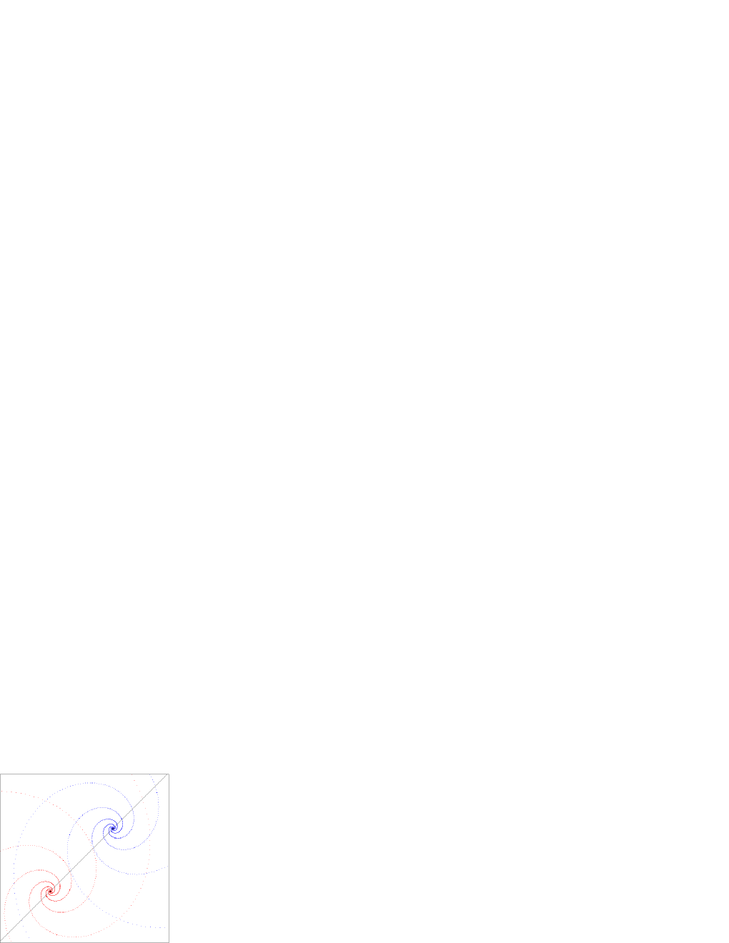
Figure 1. Spiral CT in a case of PN interaction ($S_{x}=0,999999;S_{y}$ = 0,99; $x_{0}$ = 0,9; $y_{0}$= 0,9; zoom: 28419).

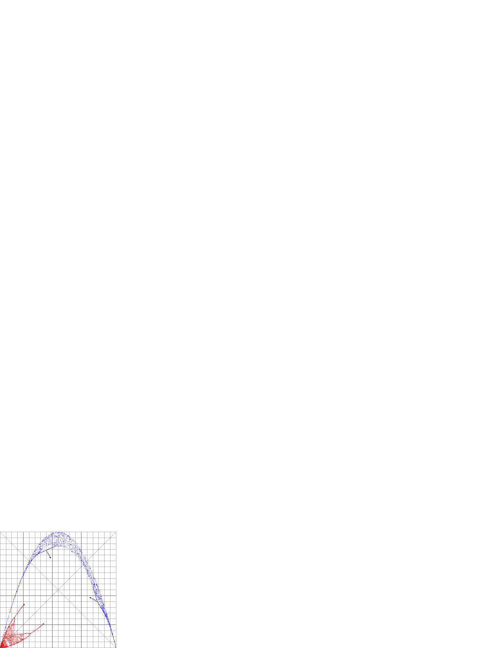
Figure 2. Left: From Chaos to order in a NN interaction ($S_{x}$ = 0,9998; $S_{y}$ = 0,999; $x_{0}$ = 0,001; $y_{0}$ = 0,9). Initially both systems evolve in a chaotic regime -parabolic regions- and then, after some thousands interactions, they evolve through their respective symmetrical coevolution trajectories towards a final 2-period attractor.

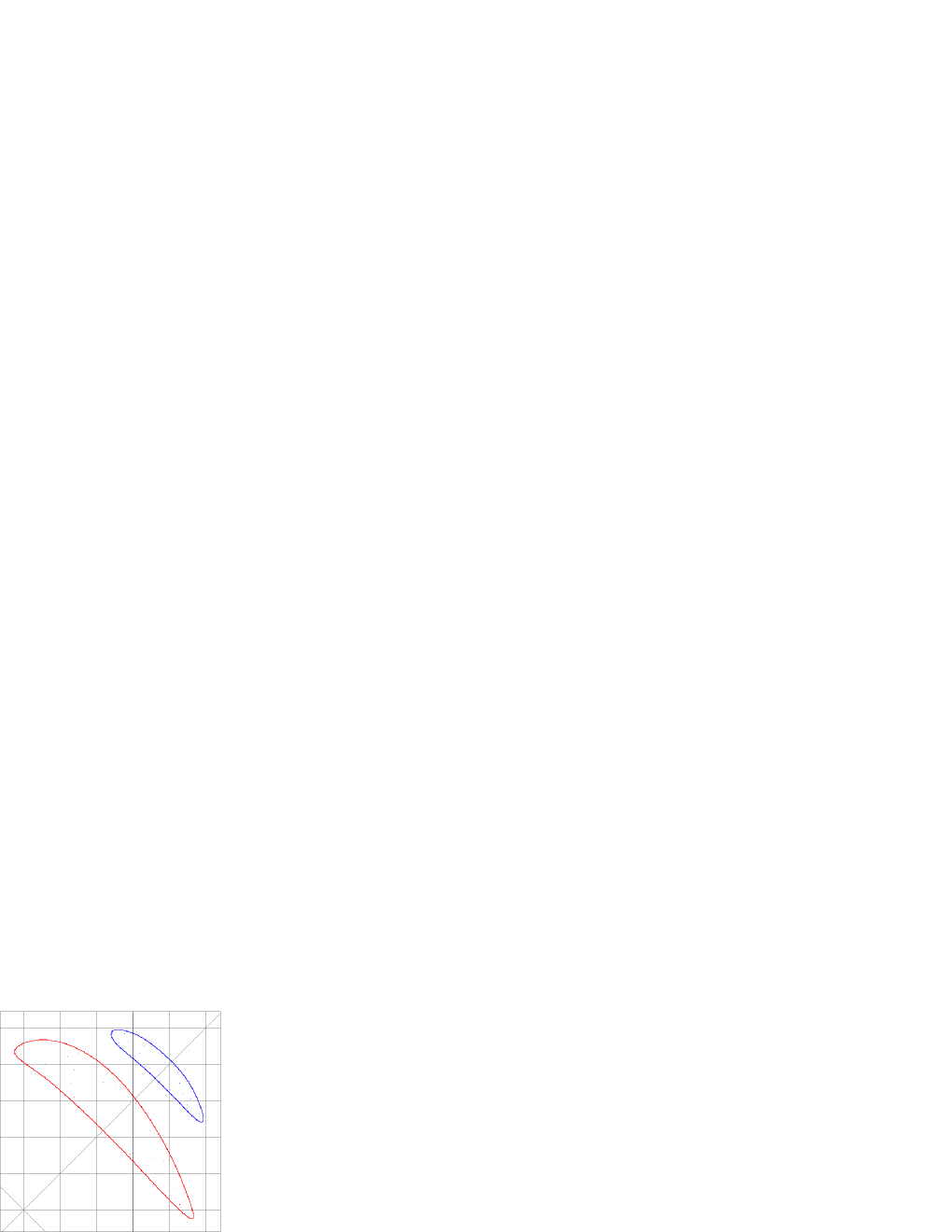
Figure 3. Orbital attractor of single orbit in he interaction defined by $S_{x}$ = 0,988; $S_{y}$ = 0,3; $x_{0}$ = 0,9; $y_{0}$ = 0,9; zoom: 4.

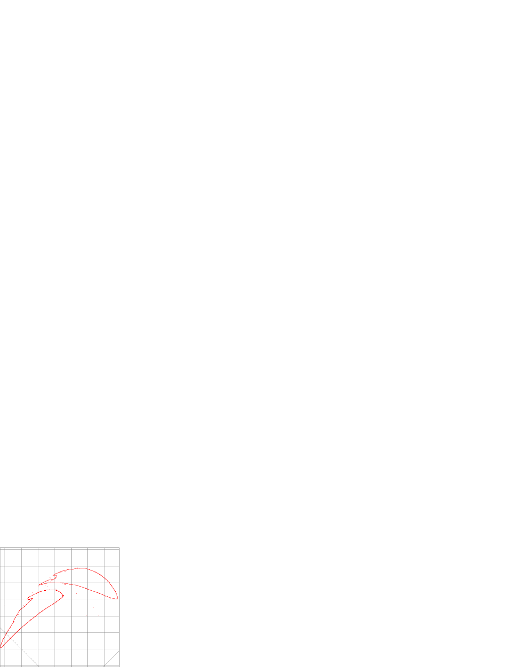
Figure 4. Orbital attractor of irregular orbit. NN interaction $S_{x}$ = 0,335; $S_{y}$ = 0,333; $x_{0}$ = 0,3; $y_{0}$ = 0,2; zoom: 3.

Figure 5. Orbital attractors of irregular orbit. PN interaction $S_{x}$ = 0,9999; $S_{y}$ = 0,23308; $x_{0}$ = 0,2; $y_{0}$ = 0,4; zoom: 13.

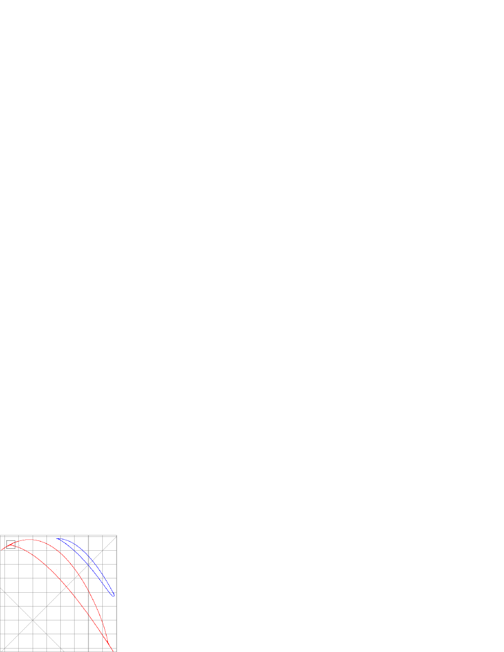
Figure 6. Orbital attractor of folded orbit corresponding to the PN interaction $S_{x}$ = 0,999; $S_{y}$ = 0,232; $x_{0}$ = 0,9; $y_{0}$ = 0,9; zoom: 3

Figure 7. Complex region of an orbital attractor of folded orbit corresponding to the PN interaction $S_{x}$ = 0,999; $S_{y}$ = 0,232; $x_{0}$ = 0,9; $y_{0}$ = 0,9; zoom: 97.

Figure 8. Diagonal symmetry towards a final period-16 attractor corresponding to the NN interaction defined by $S_{x}$ = 0.99988; $S_{y}$ = 0.9976; $x_{0}$ = 0.765; $y_{0}$ = 0.234; zoom: 2.

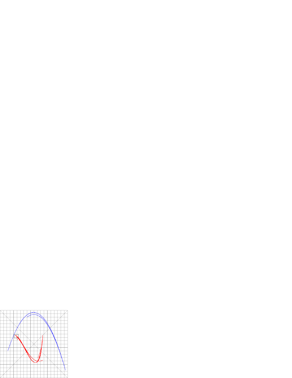
Figure 9. Fractal orbital corresponding to the NN interaction $S_{x}$ = 0.8; $S_{y}$ = 0.1; $x_{0}$ = 0.22; $y_{0}$ = 0.12.

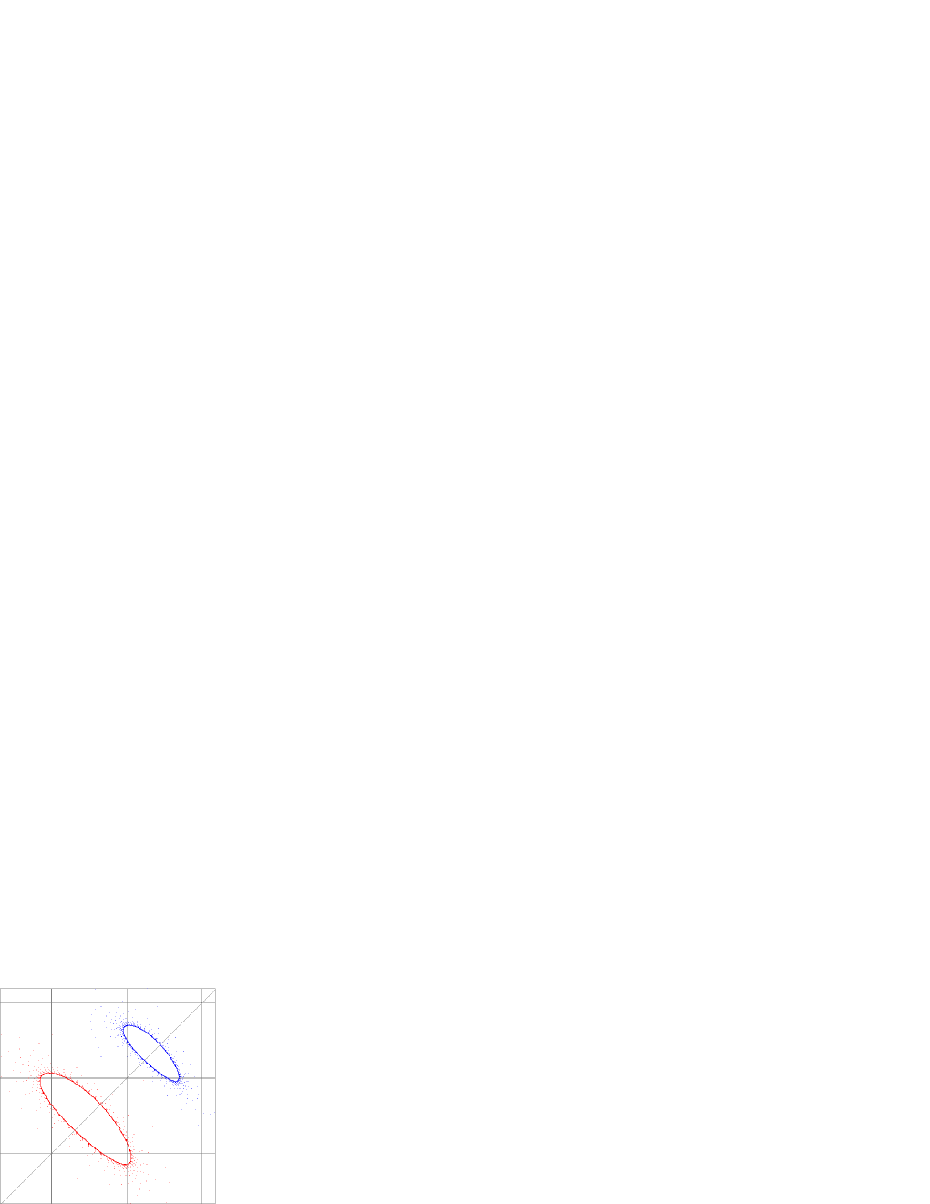
Figure 10. Radial CT towards an orbital attractor of $S_{x}$ = 0.999; $S_{y}$ = 0.393999; $x_{0}$ = 0.45; $y_{0}$ = 0.67; zoom: 7

Figure 11. Radial CT towards a period-1 attractor of the PN interaction defined by $S_{x}$ = 0.999; $S_{y}$ = 0.399; $x_{0}$ = 0.8; $y_{0}$ = 0.8. zoom: 115.

References

- [1] John Baez, The Quantum of Area?, Nature 421 (2003), 702 – 703.
- [2] Jacob D. Bekenstein, Black Hole Thermodynamics, Physics Today 33 (1980), no. 1, 24–31.
- [3] by same author, La información en un universo holográfico, Investigación y Ciencia (2003), no. 325, 36 – 43.
- [4] Jean Paul Van Bendegem, In defense of discrete space and time, Logique et Analyse 38 (1997), 150 –152.
- [5] by same author, Finitism in Geometry, Stanford Encyclopaedia of Philosophy (E. N. Zalta, ed.), Stanford University, URL = http://plato.stanford.edu, 2002.
- [6] E. Biser, Discrete Real Space, Journal of Philosophy 38 (1941), 518 – 524.
- [7] H. R. Coish, Elementary particles in a finite world geometry, Physical Review 114 (1959), 383 – 388.
- [8] Bo Deng, The Time Invariance Principle, Ecological (non)chaos, and A Fundamental Pitfall of Discrete Modeling, arXiv.q-bio (2007), 1–15.
- [9] D. Finkelstein and E. Rodríguez, Quantum time-space and gravity, Quantum Concepts in Space and Time (R. Penrose and C. J. Isham, eds.), Oxford University Press, Oxford, 1986, pp. 247 – 254.
- [10] P. Forrest, Is Space-time Discrete or Continuous?, Synthese 103 (1995), 327 – 354.
- [11] Brian Green, El universo elegante, Editorial Crítica, Barcelona, 2001.
- [12] by same author, The Fabric of the Cosmos. Space. Time. And the Texture of Reality, Alfred A. Knopf, New York, 2004.
- [13] H. Kragh and B. Carazza, From Time Atoms to Space-time Quantization: the Idea of Discrete Time, ca 1925-1936, Studies in the History and the Philosphy of Science 25 (1994), 437 – 462.
- [14] Antonio León, Más allá del caos. Una introducción a la interacción recursiva, Interciencia, http://www.interciencia.es, 2008.
- [15] Antonio León Sánchez, Coevolution: New Thermodynamic Theorems, Journal of Theoretical Biology 147 (1990), 205 – 212.
- [16] by same author, Intercalculus, http://www.interciencia.es, 2008.
- [17] Seth Loyd and Y. Jack Ng, Computación en agujeros negros, Investigación y Ciencia (Scientifc American) (2005), no. 340, 59 – 67.
- [18] Robert M. May, Simple mathematical models with very complicated dynamics, Nature 261 (1976), 459 – 467.
- [19] A. Meessen, Is it logically possible to generalize physics through space-time quantization?, Philosophie der Naturwissenschaften. Akten des 13 Internationalen Wittgenstein Symposium (P. Weingartner and G. Schurz, eds.), Hölder-Pichler-Tempsky, Vienna, 1989, pp. 19 – 47.
- [20] N Metropolis, M. L. Stein, and P. R. Stein, On finite limit sets for transformations on the unit interval, Journal of Combinatorial Theory, Series A 15 (1973), no. 1, 25–44.
- [21] Carlo Rovelli, Quantum spacetime: What do we know?, Physics meets Philosophy at the Plank scale (Craig Callender and Nick Huggett, eds.), Cambridge University Press, Cambridge, 2001, pp. 101 – 122.
- [22] Lee Smolin, Three roads to quantum gravity. A new understanding of space, time and the universe, Phoenix, London, 2003.
- [23] Lee Smolin, Átomos del espacio y del tiempo, Investigación y Ciencia (Scientifc American) (2004), no. 330, 58 – 67.
- [24] Leonard Susskind, Los agujeros negros y la paradoja de la información, Investigación y Ciencia (Scientifc American) (1997), no. 249, 12 – 18.
- [25] Stanislaw M. Ulam and Paul Stein, Non linear transformation studies on electronic computers, Rozprawy Matematyczne 39 (1963), 1–66.
- [26] Gabriele Veneziano, El universo antes de la Gran Explosión, Investigación y Ciencia (Scientifc American) (2004), no. 334, 58 – 67.