From Deterministic Chaos
to Anomalous Diffusion
Dr. habil. Rainer Klages
Queen Mary University of London
School of Mathematical Sciences
Mile End Road, London E1 4NS
e-mail: r.klages@qmul.ac.uk

Chapter 0 Introduction

Over the past few decades it was realized that deterministic dynamical systems involving only a few variables can exhibit complexity reminiscent of many-particle systems if the dynamics is chaotic, as can be quantified by the existence of a positive Ljapunov exponent [Sch89b]. Such systems provided important paradigms in order to construct a theory of nonequilibrium statistical physics starting from first principles, i.e., based on microscopic nonlinear equations of motion. This novel approach led to the discovery of fundamental relations characterizing transport in terms of deterministic chaos, of which formulas relating deterministic diffusion to differences between Ljapunov exponents and dynamical entropies form important examples [Dor99, Gas98, Kla07b]. More recently scientists learned that random-looking evolution in time and space also occurs under conditions that are weaker than requiring a positive Ljapunov exponent, which means that the separation of nearby trajectories is weaker than exponential [Kla07b]. This class of dynamical systems is called weakly chaotic and typically leads to transport processes that require descriptions going beyond standard methods of statistical mechanics. A paradigmatic example is the phenomenon of anomalous diffusion, where the mean square displacement of an ensemble of particles does not grow linearly in the long-time limit, as in case of ordinary Brownian motion, but nonlinearly in time. Such anomalous tranport phenomena do not only pose new fundamental questions to theorists but were also observed in a large number of experiments [Kla08].

This review gives a very tutorial introduction to all these topics in form of three chapters: Chapter 1 reminds of two basic concepts quantifying deterministic chaos in dynamical systems, which are Ljapunov exponents and dynamical entropies. These approaches will be illustrated by studying simple one-dimensional maps. Slight generalizations of these maps will be used in Chapter 2 in order to motivate the problem of deterministic diffusion. Their analysis will yield an exact formula expressing diffusion in terms of deterministic chaos. In the first part of Chapter 3 we further generalize these simple maps such that they exhibit anomalous diffusion. This dynamics can be analyzed by applying continuous time random walk theory, a stochastic approach that leads to generalizations of ordinary laws of diffusion of which we derive a fractional diffusion equation as an example. Finally, we demonstrate the relevance of these theoretical concepts to experiments by studying the anomalous dynamics of biological cells migration.

The degree of difficulty of the material presented increases from chapter to chapter, and the style of our presentation changes accordingly: While Chapter 1 mainly elaborates on textbook material of chaotic dynamical systems [Ott93, Bec93], Chapter 2 covers advanced topics that emerged in research over the past twenty years [Dor99, Gas98, Kla96b]. Both these chapters were successfully taught twice to first year Ph.D. students in form of five one-hour lectures. Chapter 3 covers topics that were presented by the author in two one-hour seminar talks and are closely related to recently published research articles [Kor05, Kor07, Die08].

Chapter 1 Deterministic chaos

To clarify the general setting, we start with a brief reminder about the dynamics of time-discrete one-dimensional dynamical systems. We then quantify chaos in terms of Ljapunov exponents and (metric) entropies by focusing on systems that are closed on the unit interval. These ideas are then generalized to the case of open systems, where particles can escape (in terms of absorbing boundary conditions). Most of the concepts we are going to introduce carry over, suitably generalized, to higher-dimensional and time-continuous dynamical systems.

1 Dynamics of simple maps

As a warm-up, let us recall the following:

Definition 1

Let $J\subseteq\mathbb{R},x_{n}\in J,n\in\mathbb{Z}.$ Then

$$F:J\to J\quad,\quad x_{n+1}=F(x_{n})$$ (1)

is called a one-dimensional time-discrete map. $x_{n+1}=F(x_{n})$ are sometimes called the equations of motion of the dynamical system.

Choosing the initial condition $x_{0}$ determines the outcome after $n$ discrete time steps, hence we speak of a deterministic dynamical system. It works as follows:

$$x_{1} = F(x_{0})=F^{1}(x_{0}),$$

$$x_{2} = F(x_{1})=F(F(x_{0}))=F^{2}(x_{0}).$$

$$\Rightarrow\>F^{m}(x_{0}):=\underbrace{F\circ F\circ\cdots F(x_{0})}_{\mbox{m-fold composed map}}\quad.$$ (2)

In other words, there exists a unique solution to the equations of motion in form of $x_{n}=F(x_{n-1})=\ldots=F^{n}(x_{0})$, which is the counterpart of the flow for time-continuous systems. In the first two chapters we will focus on simple piecewise linear maps. The following one serves as a paradigmatic example [Sch89b, Ott93, All97, Dor99]:

Example 1

The Bernoulli shift (also shift map, doubling map, dyadic transformation)

Figure 1: The Bernoulli shift.

The Bernoulli shift shown in Fig. 1 can be defined by

$$B:[0,1)\to[0,1)\;,\;B(x):=2x\;\mbox{mod 1}\;=\left\{\begin{array}[]{l}2x\;,\;0\leq x<1/2\\ 2x-1\;,\;1/2\leq x<1\end{array}\right.\quad.$$ (3)

One may think about the dynamics of such maps as follows, see Fig. 2: Assume we fill the whole unit interval with a uniform distribution of points. We may now decompose the action of the Bernoulli shift into two steps:

1. The map stretches the whole distribution of points by a factor of two, which leads to divergence of nearby trajectories.

2. Then we cut the resulting line segment in the middle due to the the modulo operation $\mod 1$, which leads to motion bounded on the unit interval.

Figure 2: Stretch-and-cut mechanism in the Bernoulli shift.

The Bernoulli shift thus yields a simple example for an essentially nonlinear stretch-and-cut mechanism, as it typically generates deterministic chaos [Ott93]. Such basic mechanisms are also encountered in more realistic dynamical systems. We may remark that ‘stretch and fold’ or ‘stretch, twist and fold’ provide alternative mechanisms for generating chaotic behavior, see, e.g., the tent map. The reader may wish to play around with these ideas in thought experiments, where the sets of points is replaced by kneading dough. These ideas can be made mathematically precise in form of what is called mixing in dynamical systems, which is an important concept in the ergodic theory of dynamical systems [Arn68, Dor99].

2 Ljapunov chaos

In Ref. [Dev89] Devaney defines chaos by requiring that for a given dynamical system three conditions have to be fulfilled: sensitivity, existence of a dense orbit, and that the periodic points are dense. The Ljapunov exponent generalizes the concept of sensitivity in form of a quantity that can be calculated more conveniently, as we will motivate by an example:

Example 2

Ljapunov instability of the Bernoulli shift [Ott93, Rob95]

Consider two points that are initially displaced from each other by $\delta x_{0}:=|x_{0}^{\prime}-x_{0}|$ with $\delta x_{0}$ “infinitesimally small” such that $x_{0},x_{0}^{\prime}$ do not hit different branches of the Bernoulli shift $B(x)$ around $x=1/2$. We then have

$$\delta x_{n}:=|x_{n}^{\prime}-x_{n}|=2\delta x_{n-1}=2^{2}\delta x_{n-2}=\ldots=2^{n}\delta x_{0}=e^{n\ln 2}\delta x_{0}\quad.$$ (4)

We thus see that there is an exponential separation between two nearby points as we follow their trajectories. The rate of separation $\lambda(x_{0}):=\ln 2$ is called the (local) Ljapunov exponent of the map $B(x)$.

This simple example can be generalized as follows, leading to the general definition of the Ljapunov exponent for one-dimensional maps $F$. Consider

$$\delta x_{n}=|x_{n}^{\prime}-x_{n}|=|F^{n}(x_{0}^{\prime})-F^{n}(x_{0})|=:\delta x_{0}e^{n\lambda(x_{0})}\>(\delta x_{0}\to 0)$$ (5)

for which we presuppose that an exponential separation of trajectories exists. By furthermore assuming that $F$ is differentiable we can rewrite this equation to

$$\lambda(x_{0}) = \lim_{n\to\infty}\lim_{\delta x_{0}\to 0}\frac{1}{n}\ln\frac{\delta x_{n}}{\delta x_{0}}$$ (6)

$$= \lim_{n\to\infty}\lim_{\delta x_{0}\to 0}\frac{1}{n}\ln\frac{\left|F^{n}(x_{0}+\delta x_{0})-F^{n}(x_{0})\right|}{\delta x_{0}}$$

$$= \lim_{n\to\infty}\frac{1}{n}\ln\left|\frac{dF^{n}(x)}{dx}\right|_{x=x_{0}}\quad.$$

Using the chain rule we obtain

$$\left.\frac{\mathrm{d}F^{n}(x)}{\mathrm{d}x}\right|_{x=x_{0}}=F^{\prime}(x_{n-1})F^{\prime}(x_{n-2})\ldots F^{\prime}(x_{0})\quad,$$ (7)

which leads to

$$\lambda(x_{0}) = \lim_{n\to\infty}\frac{1}{n}\ln\left|\prod_{i=0}^{n-1}F^{\prime}(x_{i})\right|$$ (8)

$$= \lim_{n\to\infty}\frac{1}{n}\sum_{i=0}^{n-1}\ln\left|F^{\prime}(x_{i})\right|\quad.$$

This simple calculation motivates the following definition:

Definition 2

[All97] Let $F\in C^{1}$ be a map of the real line. The local Ljapunov exponent $\lambda(x_{0})$ is defined as

$$\lambda(x_{0}):=\lim_{n\to\infty}\frac{1}{n}\sum_{i=0}^{n-1}\ln\left|F^{\prime}(x_{i})\right|$$ (9)

if this limit exists.

Remark 1

1. If $F$ is not $C^{1}$ but piecewise $C^{1}$, the definition can still be applied by excluding single points of non-differentiability.

2. If $F^{\prime}(x_{i})=0\Rightarrow\not\exists\lambda(x)$. However, usually this concerns only an ‘atypical’ set of points.

Example 3

For the Bernoulli shift $B(x)=2x\mod 1$ we have $B^{\prime}(x)=2\>\forall x\in[0,1)\>,\>x\neq\frac{1}{2}$, hence trivially

$$\lambda(x)=\frac{1}{n}\sum_{k=0}^{n-1}\ln 2=\ln 2$$ (10)

at these points.

Note that Definition 2 defines the local Ljapunov exponent $\lambda(x_{0})$, that is, this quantity may depend on our choice of initial conditions $x_{0}$. For the Bernoulli shift this is not the case, because this map has a uniform slope of two except at the point of discontinuity, which makes the calculation trivial. Generally the situation is more complicated. One question is then of how to calculate the local Ljapunov exponent, and another one to which extent it depends on initial conditions. An answer to both these questions is provided in form of the global Ljapunov exponent that we are going to introduce, which does not depend on initial conditions and thus characterizes the stability of the map as a whole.

It is introduced by observing that the local Ljapunov exponent in Definition 2 is defined in form of a time average, where $n$ terms along the trajectory with initial condition $x_{0}$ are summed up by averaging over $n$. That this is not the only possibility to define an average quantity is clarified by the following definition:

Definition 3

time and ensemble average [Dor99, Arn68]

Let $\mu^{*}$ be the invariant probability measure of a one-dimensional map $F$ acting on $J\subseteq\mathbb{R}$. Let us consider a function $g:J\to\mathbb{R}$, which we may call an “observable”. Then

$$\overline{g(x)}:=\lim_{n\to\infty}\frac{1}{n}\sum_{k=0}^{n-1}g(x_{k})\quad,$$ (11)

$x=x_{0}$, is called the time (or Birkhoff) average of $g$ with respect to $F$.

$$\langle g\rangle:=\int_{J}d\mu^{*}g(x)$$ (12)

where, if such a measure exists, $d\mu^{*}=\rho^{*}(x)\>dx$, is called the ensemble (or space) average of $g$ with respect to $F$. Here $\rho^{*}(x)$ is the invariant density of the map, and $d\mu^{*}$ is the associated invariant measure [Ott93, Las94, Kla07a]. Note that $\overline{g(x)}$ may depend on $x$, whereas $\langle g\rangle$ does not.

If we choose $g(x)=\ln|F^{\prime}(x)|$ as the observable in Eq. (11) we recover Definition 2 for the local Ljapunov exponent,

$$\lambda(x):=\overline{\ln|F^{\prime}(x)|}=\lim_{n\to\infty}\frac{1}{n}\sum_{k=0}^{n-1}\ln|F^{\prime}(x_{k})|\quad,$$ (13)

which we may write as $\lambda_{t}(x)=\lambda(x)$ in order to label it as a time average. If we choose the same observable for the ensemble average Eq. (12) we obtain

$$\lambda_{e}:=\langle\ln|F^{\prime}(x)|\rangle:=\int_{J}dx{\rho^{*}(x)}\ln|F^{\prime}(x)|\quad.$$ (14)

Example 4

For the Bernoulli shift we have seen that for almost every $x\in[0,1)$ $\lambda_{t}=\ln 2$. For $\lambda_{e}$ we obtain

$$\lambda_{e}=\int_{0}^{1}dx\rho^{*}(x)\ln 2=\ln 2\quad,$$ (15)

taking into account that $\rho^{*}(x)=1$, as you have seen before. In other words, time and ensemble average are the same for almost every $x$,

$$\lambda_{t}(x)=\lambda_{e}=\ln 2\quad.$$ (16)

This motivates the following fundamental definition:

Definition 4

ergodicity [Arn68, Dor99]

A dynamical system is called ergodic if for every $g$ on $J\subseteq\mathbb{R}$ satisfying $\int d\mu^{*}\>|g(x)|<\infty$

$$\overline{g(x)}=\langle g\rangle$$ (17)

for typical $x$.

For our purpose it suffices to think of a typical $x$ as a point that is randomly drawn from the invariant density $\rho^{*}(x)$. This definition implies that for ergodic dynamical systems $\overline{g(x)}$ does not depend on $x$. That the time average is constant is sometimes also taken as a definition of ergodicity [Dor99, Bec93]. To prove that a given system is ergodic is typically a hard task and one of the fundamental problems in the ergodic theory of dynamical systems; see [Arn68, Dor99, Tod92] for proofs of ergodicity in case of some simple examples.

On this basis, let us get back to Ljapunov exponents. For time average $\lambda_{t}(x)$ and ensemble average $\lambda_{e}$ of the Bernoulli shift we have found that $\lambda_{t}(x)=\lambda_{e}=\ln 2$. Definition 4 now states that the first equality must hold whenever a map $F$ is ergodic. This means, in turn, that for an ergodic dynamical system the Ljapunov exponent becomes a global quantity characterizing a given map $F$ for a typical point $x$ irrespective of what value we choose for the initial condition, $\lambda_{t}(x)=\lambda_{e}=\lambda$. This observation very much facilitates the calculation of $\lambda$, as is demonstrated by the following example:

Example 5

Let us consider the map $A(x)$ displayed in Fig. 3 below:

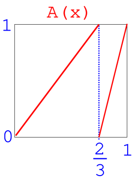
Figure 3: A simple map for demonstrating the calculation of Ljapunov exponents via ensemble averages.

From the figure we can infer that

$$A(x):=\left\{\begin{array}[]{l}\frac{3}{2}x\;,\;0\leq x<\frac{2}{3}\\ 3x-2\;,\;\frac{2}{3}\leq x<1\end{array}\right.\quad.$$ (18)

It is not hard to see that the invariant probability density of this map is uniform, $\rho^{*}(x)=1$. The Ljapunov exponent $\lambda$ for this map is then trivially calculated to

$$\lambda=\int_{0}^{1}\mathrm{d}x\rho^{*}(x)\ln|A^{\prime}(x)|=\ln 3-\frac{2}{3}\ln 2\quad.$$ (19)

By assuming that map $A$ is ergodic (which here is the case), we can conclude that this result for $\lambda$ represents the value for typical points in the domain of $A$.

In other words, for an ergodic map the global Ljapunov exponent $\lambda$ yields a number that assesses whether it is chaotic in the sense of exhibiting an exponential dynamical instability. This motivates the following definition of deterministic chaos:

Definition 5

Chaos in the sense of Ljapunov [Rob95, Ott93, All97, Bec93]

An ergodic map $F:J\to J,\>J\subseteq\mathbb{R},\>F$ (piecewise) $C^{1}$ is said to be L-chaotic on $J$ if $\lambda>0$.

Why did we introduce a definition of chaos that is different from Devaney’s definition mentioned earlier? One reason is that often the largest Ljapunov exponent of a dynamical system is easier to calculate than checking for sensitivity. Furthermore, the magnitude of the positive Ljapunov exponent quantifies the strength of chaos. This is the reason why in the applied sciences “chaos in the sense of Ljapunov” became a very popular concept. Note that there is no unique quantifier of deterministic chaos. Many different definitions are available highlighting different aspects of “chaotic behavior”, all having their advantages and disadvantages. The detailed relations between them (such as the ones between Ljapunov and Devaney chaos) are usually non-trivial and a topic of ongoing research [Kla07a]. We will encounter yet another definition of chaos in the following section.

3 Entropies

This section particularly builds upon the presentations in [Ott93, Dor99]; for a more mathematical approach see [Eck85]. Let us start with a brief motivation outlining the basic idea of entropy production in dynamical systems. Consider again the Bernoulli shift by decomposing its domain $J=[0,1)$ into $J_{0}:=[0,1/2)$ and $J_{1}:=[1/2,1)$. For $x\in[0,1)$ define the output map $s$ by [Sch89b]

$$s:[0,1)\to\{0,1\}\;,\;s(x):=\left\{\begin{array}[]{l}0\;,\;x\in J_{0}\\ 1\;,\;x\in J_{1}\end{array}\right.$$ (22)

and let $s_{n+1}:=s(x_{n})$. Now choose some initial condition $x_{0}\in J$. According to the above rule we obtain a digit $s_{1}\in\{0,1\}$. Iterating the Bernoulli shift according to $x_{n+1}=B(x_{n})$ then generates a sequence of digits $\{s_{1},s_{2},\ldots,s_{n}\}$. This sequence yields nothing else than the binary representation of the given initial condition $x_{0}$ [Sch89b, Ott93, Dor99]. If we assume that we pick an initial condition $x_{0}$ at random and feed it into our map without knowing about its precise value, this simple algorithm enables us to find out what number we have actually chosen. In other words, here we have a mechanism of creation of information about the initial condition $x_{0}$ by analyzing the chaotic orbit generated from it as time evolves.

Conversely, if we now assume that we already knew the initial state up to, say, $m$ digits precision and we iterate $p>m$ times, we see that the map simultaneously destroys information about the current and future states, in terms of digits, as time evolves. So creation of information about previous states goes along with loss of information about current and future states. This process is quantified by the Kolmogorov-Sinai (KS) entropy (also called metric, or measure-theoretic entropy), which measures the exponential rate at which information is produced, respectively lost in a dynamical system, as we will see below.

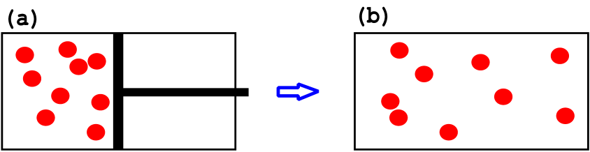
Figure 4: Schematic representation of a gas of molecules in a box. In (a) the gas is constrained by a piston to the left hand side of the box, in (b) the piston is removed and the gas can spread out over the whole box. This illustrates the basic idea of (physical) entropy production.

The situation is similar to the following thought experiment illustrated in Fig. 4: Let us assume we have a gas consisting of molecules, depicted as billiard balls, which is constrained to the left half of the box as shown in (a). This is like having some information about the initial conditions of all gas molecules, which are in a more localized, or ordered, state. If we remove the piston as in (b), we observe that the gas spreads out over the full box until it reaches a uniform equilibrium steady state. We then have less information available about the actual positions of all gas molecules, that is, we have increased the disorder of the whole system. This observation lies at the heart of what is called thermodynamic entropy production in the statistical physics of many-particle systems which, however, is usually assessed by quantities that are different from the KS-entropy [Fal05].

At this point we may not further elaborate on the relation to statistical physical theories. Instead, let us make precise what we mean by KS-entropy starting from the famous Shannon (or information) entropy [Ott93, Bec93]. This entropy is defined as

$$H_{S}:=\sum_{i=1}^{r}p_{i}\ln\left(\frac{1}{p_{i}}\right)\quad,$$ (23)

where $p_{i}\>,\>i=1,\ldots,r$ are the probabilities for the $r$ possible outcomes of an experiment. Think, for example, of a roulette game, where carrying out the experiment one time corresponds to $n=1$ in the iteration of an unknown map. $H_{S}$ then measures the amount of uncertainty concerning the outcome of the experiment, which can be understood as follows:

1. Let $p_{1}=1\>,\>p_{i}=0$ otherwise. By defining $p_{i}\ln\left(\frac{1}{p_{i}}\right):=0\>,\>i\neq 1,$ we have $H_{S}=0$. This value of the Shannon entropy must therefore characterize the situation where the outcome is completely certain.

2. Let $p_{i}=1/r\>,\>i=1,2,\ldots,r$. Then we obtain $H_{S}=\ln r$ thus characterizing the situation where the outcome is most uncertain because of equal probabilities.

Case (1) thus represents the situation of no information gain by doing the experiment, case (2) corresponds to maximum information gain. These two special cases must therefore define the lower and upper bounds of $H_{S}$,

$$0\leq H_{S}\leq\ln r\quad.$$ (24)

This basic concept of information theory carries over to dynamical systems by identifying the probabilities $p_{i}$ with invariant probability measures $\mu_{i}^{*}$ on subintervals of a given dynamical system’s phase space. The precise connection is worked out in four steps [Ott93, Dor99]:

1. Partition and refinement:

Consider a map $F$ acting on $J\subseteq\mathbb{R}$, and let $\mu^{*}$ be an invariant probability measure generated by the map. Let $\{J_{i}\},\ i=1,\ldots,s$ be a partition of $J$. We now construct a refinement of this partition as illustrated by the following example:

Example 6

Consider the Bernoulli shift displayed in Fig. 5. Start with the partition $\{J_{0},J_{1}\}$ shown in (a). Now create a refined partition by iterating these two partition parts backwards according to $B^{-1}(J_{i})$ as indicated in (b). Alternatively, you may take the second forward iterate $B^{2}(x)$ of the Bernoulli shift and then identify the preimages of $x=1/2$ for this map. In either case the new partition parts are obtained to

$$J_{00} := \{x:x\in J_{0}\>,\>B(x)\in J_{0}\}$$

$$J_{01} := \{x:x\in J_{0}\>,\>B(x)\in J_{1}\}$$

$$J_{10} := \{x:x\in J_{1}\>,\>B(x)\in J_{0}\}$$

$$J_{11} := \{x:x\in J_{1}\>,\>B(x)\in J_{1}\}\quad.$$ (25)

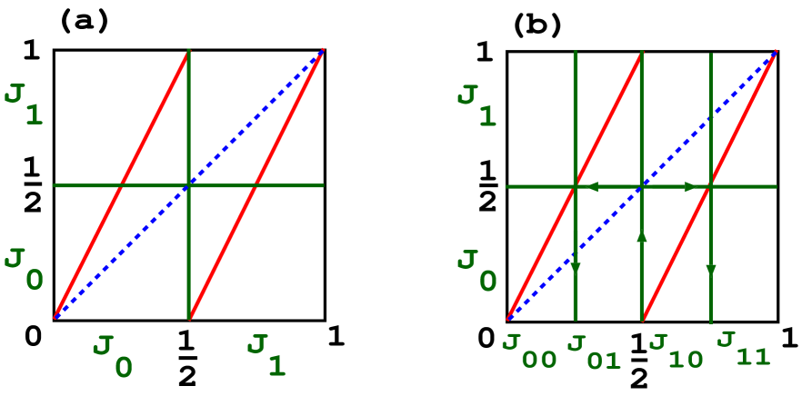
Figure 5: (a) The Bernoulli shift and a partition of the unit interval consisting of two parts. (b) Refinement of this partition under backward iteration.

If we choose $x_{0}\in J_{00}$ we thus know in advance that the orbit emerging from this initial condition under iteration of the map will remain in $J_{0}$ at the next iteration. That way, the refined partition clearly yields more information about the dynamics of single orbits.

More generally, for a given map $F$ the above procedure is equivalent to defining

$$\{J_{i_{1}i_{2}}\}:=\{J_{i_{1}}\cap F^{-1}(J_{i_{2}})\}\quad.$$ (26)

The next round of refinement proceeds along the same lines yielding

$$\{J_{i_{1}i_{2}i_{3}}\}:=\{J_{i_{1}}\cap F^{-1}(J_{i_{2}})\cap F^{-2}(J_{i_{3}})\}\quad,$$ (27)

and so on. For convenience we define

$$\{J_{i}^{n}\}:=\{J_{i_{1}i_{2}\ldots i_{n}}\}=\{J_{i_{1}}\cap F^{-1}(J_{i_{2}})\cap\ldots\cap F^{-(n-1)}(J_{i_{n}})\}\quad.$$ (28)

2. H-function:

In analogy to the Shannon entropy Eq. (23) next we define the function

$$H(\{J_{i}^{n}\}):=-\sum_{i}\mu^{*}(J_{i}^{n})\ln\mu^{*}(J_{i}^{n})\quad,$$ (29)

where $\mu^{*}(J_{i}^{n})$ is the invariant measure of the map $F$ on the partition part $J_{i}^{n}$ of the $n$th refinement.

Example 7

For the Bernoulli shift with uniform invariant probability density $\rho^{*}(x)=1$ and associated (Lebesgue) measure $\mu^{*}(J_{i}^{n})=\int_{J_{i}^{n}}dx\>\rho^{*}(x)=\mbox{diam}\left(J_{i}^{n}\right)$ we can calculate

$$H(\{J_{i}^{1}\}) = -(\frac{1}{2}\ln\frac{1}{2}+\frac{1}{2}\ln\frac{1}{2})=\ln 2$$

$$H(\{J_{i}^{2}\}) = H(\{J_{i_{1}}\cap B^{-1}(J_{i_{2}})\})=-4(\frac{1}{4}\ln\frac{1}{4})=\ln 4$$

$$H(\{J_{i}^{3}\}) = \ldots=\ln 8=\ln 2^{3}$$

$$\vdots$$

$$H(\{J_{i}^{n}\}) = \ln 2^{n}$$ (30)

3. Take the limit:

We now look at what we obtain in the limit of infinitely refined partition by

$$h(\{J_{i}^{n}\}):=\lim_{n\to\infty}\frac{1}{n}H(\{J_{i}^{n}\})\quad,$$ (31)

which defines the rate of gain of information over $n$ refinements.

Example 8

For the Bernoulli shift we trivially obtain

$$h(\{J_{i}^{n}\})=\ln 2\quad.$$ (32)

4. Supremum over partitions:

We finish the definition of the KS-entropy by maximizing $h(\{J_{i}^{n}\})$ over all available partitions,

$$h_{KS}:=\sup_{\{J_{i}^{n}\}}h(\{J_{i}^{n}\})\quad.$$ (33)

The last step can be avoided if the partition $\{J_{i}^{n}\}$ is generating for which it must hold that $\mbox{diam}\left(J_{i}^{n}\right)\to 0\;(n\to\infty)$ [Eck85, Kat95, Bad97]. It is quite obvious that for the Bernoulli shift the partition chosen above is generating in that sense, hence $h_{KS}=\ln 2$ for this map.

Remark 2

[Sch89b]

1. For strictly periodic motion there is no refinement of partition parts under backward iteration, hence $h_{KS}=0$; see, for example, the identity map $I(x)=x$.

2. For stochastic systems all preimages are possible, so there is immediately an infinite refinement of partition parts under backward iteration, which leads to $h_{KS}\to\infty$.

These considerations suggest yet another definition of deterministic chaos:

Definition 6

Measure-theoretic chaos [Bec93]

A map $F:J\to J,\>J\subseteq\mathbb{R},$ is said to be chaotic in the sense of exhibiting dynamical randomness if $h_{KS}>0$.

Again, one may wonder about the relation between this new definition and our previous one in terms of Ljapunov chaos. Let us look again at the Bernoulli shift:

Example 9

For $B(x)$ we have calculated the Ljapunov exponent to $\lambda=\ln 2$, see Example 4. Above we have seen that $h_{KS}=\ln 2$ for this map, so we arrive at $\lambda=h_{KS}=\ln 2$.

That this equality is not an artefact due to the simplicity of our chosen model is stated by the following theorem:

Theorem 1

Pesin’s Theorem (1977) [Dor99, Eck85, You02]

For closed $C^{2}$ Anosov systems the KS-entropy is equal to the sum of positive Ljapunov exponents.

A proof of this theorem goes considerably beyond the scope of this course [You02]. In the given formulation it applies to higher-dimensional dynamical systems that are “suitably well-behaved” in the sense of exhibiting the Anosov property. Applied to one-dimensional maps, it means that if we consider transformations which are “closed” by mapping an interval onto itself, $F:\>J\to J$, under certain conditions (which we do not further specify here) and if there is a positive Ljapunov exponent $\lambda>0$ we can expect that $\lambda=h_{KS}$, as we have seen for the Bernoulli shift. In fact, the Bernoulli shift provides an example of a map that does not fulfill the conditions of the above theorem precisely. However, the theorem can also be formulated under weaker assumptions, and it is believed to hold for an even wider class of dynamical systems.

In order to get an intuition why this theorem should hold, let us look at the information creation in a simple one-dimensional map such as the Bernoulli shift by considering two orbits $\{x_{k}\}_{k=0}^{n}$, $\{x^{\prime}_{k}\}_{k=0}^{n}$ starting at nearby initial conditions $|x_{0}^{\prime}-x_{0}|\leq\delta x_{0}\>,\>\delta x_{0}\ll 1$. Recall the encoding defined by Eq. (22). Under the first $m$ iterations these two orbits will then produce the very same sequences of symbols $\{s_{k}\}_{k=1}^{m}$, $\{s^{\prime}_{k}\}_{k=1}^{m}$, that is, we cannot distinguish them from each other by our encoding. However, due to the ongoing stretching of the initial displacement $\delta x_{0}$ by a factor of two, eventually there will be an $m$ such that starting from $p>m$ iterations different symbol sequences are generated. Thus we can be sure that in the limit of $n\to\infty$ we will be able to distinguish initially arbitrarily close orbits. If you like analogies, you may think of extracting information about the different initial states via the stretching produced by the iteration process like using a magnifying glass. Therefore, under iteration the exponential rate of separation of nearby trajectories, which is quantified by the positive Ljapunov exponent, must be equal to the rate of information generated, which in turn is given by the KS-entropy. This is at the heart of Pesin’s theorem.

We may remark that typically the KS-entropy is much harder to calculate for a given dynamical system than positive Ljapunov exponents. Hence, Pesin’s theorem is often employed in the literature for indirectly calculating the KS-entropy. Furthermore, here we have described only one type of entropy for dynamical systems. It should be noted that the concept of the KS-entropy can straightforwardly be generalized leading to a whole spectrum of Renyi entropies, which can then be identified with topological, metric, correlation and other higher-order entropies [Bec93].

4 Open systems, fractals and escape rates

This section draws particularly on [Ott93, Dor99]. So far we have only studied closed systems, where intervals are mapped onto themselves. Let us now consider an open system, where points can leave the unit interval by never coming back to it. Consequently, in contrast to closed systems the total number of points is not conserved anymore. This situation can be modeled by a slightly generalized example of the Bernoulli shift.

Example 10

In the following we will study the map

$$B_{a}:[0,1)\to[1-a/2,a/2)\;,\;B_{a}(x):=\left\{\begin{array}[]{l}ax\;,\;0\leq x<1/2\\ ax+1-a\;,\;1/2\leq x<1\end{array}\right.\quad,$$ (34)

see Fig. 6, where the slope $a\geq 2$ defines a control parameter. For $a=2$ we recover our familiar Bernoulli shift, whereas for $a>2$ the map defines an open system. That is, whenever points are mapped into the escape region of width $\Delta$ these points are removed from the unit interval. You may thus think of the escape region as a subinterval that absorbs any particles mapped onto it.

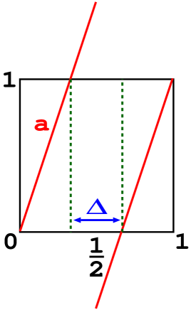
Figure 6: A generalization of the Bernoulli shift, defined as a parameter-dependent map $B_{a}(x)$ modeling an open system. The slope $a$ defines a control parameter, $\Delta$ denotes the width of the escape region.

We now wish to compute the number of points $N_{n}$ remaining on the unit interval at time step $n$, where we start from a uniform distribution of $N_{0}=N$ points on this interval at $n=0$. This can be done as follows: Recall that the probability density $\rho_{n}(x)$ was defined by

$$\rho_{n}(x):=\frac{\mbox{number of points}\>N_{n,j}\>\mbox{in interval dx centered around position}\>x_{j}\>\mbox{at time step}\>n}{\mbox{total number of points}\>N\>\mbox{times width dx}}\quad,$$ (35)

where $N_{n}=\sum_{j}N_{n,j}$. With this we have that

$$N_{1}=N_{0}-\rho_{0}N\Delta\quad.$$ (36)

By observing that for $B_{a}(x)$, starting from $\rho_{0}=1$ points are always uniformly distributed on the unit interval at subsequent iterations, we can derive an equation for the density $\rho_{1}$ of points covering the unit interval at the next time step $n=1$. For this purpose we divide the above equation by the total number of points $N$ (multiplied with the total width of the unit interval, which however is one), which yields

$$\rho_{1}=\frac{N_{1}}{N}=\rho_{0}-\rho_{0}\Delta=\rho_{0}(1-\Delta)\quad.$$ (37)

This procedure can be reiterated starting now from

$$N_{2}=N_{1}-\rho_{1}N\Delta$$ (38)

leading to

$$\rho_{2}=\frac{N_{2}}{N}=\rho_{1}(1-\Delta)\quad,$$ (39)

and so on. For general $n$ we thus obtain

$$\rho_{n}=\rho_{n-1}(1-\Delta)=\rho_{0}(1-\Delta)^{n}=\rho_{0}e^{n\ln(1-\Delta)}\quad,$$ (40)

or correspondingly

$$N_{n}=N_{0}e^{n\ln(1-\Delta)}\quad,$$ (41)

which suggests the following definition:

Definition 7

For an open system with exponential decrease of the number of points,

$$N_{n}=N_{0}e^{-\gamma n}\quad,$$ (42)

$\gamma$ is called the escape rate.

In case of our mapping we thus identify

$$\gamma=\ln\frac{1}{1-\Delta}$$ (43)

as the escape rate. We may now wonder whether there are any initial conditions that never leave the unit interval and about the character of this set of points. The set can be constructed as exemplified for $B_{a}(x)\>,\>a=3$ in Fig. 7.

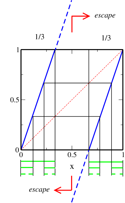
Figure 7: Construction of the set ${\cal C}_{B_{3}}$ of initial conditions of the map $B_{3}(x)$ that never leave the unit interval.

Example 11

Let us start again with a uniform distribution of points on the unit interval. We can then see that the points which remain on the unit interval after one iteration of the map form two sets, each of length $1/3$. Iterating now the boundary points of the escape region backwards in time according to $x_{n}=B_{3}^{-1}(x_{n+1})$, we can obtain all preimages of the escape region. We find that initial points which remain on the unit interval after two iterations belong to four smaller sets, each of length $1/9$, as depicted at the bottom of Fig. 7. Repeating this procedure infinitely many times reveals that the points which never leave the unit interval form the very special set ${\cal C}_{B_{3}}$, which is known as the middle third Cantor set.

Definition 8

Cantor set [Ott93, Dev89]

A Cantor set is a closed set which consists entirely of boundary points each of which is a limit point of the set.

Let us explore some fundamental properties of the set ${\cal C}_{B_{3}}$ [Ott93]:

1. From Fig. 7 we can infer that the total length $l_{n}$ of the intervals of points remaining on the unit interval after $n$ iterations, which is identical with the Lebesgue measure $\mu_{L}$ of these sets, is

   $$l_{0}=1\>,\>l_{1}=\frac{2}{3}\>,\>l_{2}=\frac{4}{9}=\left(\frac{2}{3}\right)^{2}\>,\ldots,l_{n}=\left(\frac{2}{3}\right)^{n}\quad.$$ (44)

   We thus see that

   $$l_{n}=\left(\frac{2}{3}\right)^{n}\to 0\>(n\to\infty)\quad,$$ (45)

   that is, the total length of this set goes to zero, $\mu_{L}({\cal C}_{B_{3}})=0$. However, there exist also Cantor sets whose Lebesgue measure is larger than zero [Ott93]. Note that matching $l_{n}=\exp(-n\ln(3/2))$ to Eq. (43) yields an escape rate of $\gamma=\ln(3/2)$ for this map.

2. By using the binary encoding Eq. (22) for all intervals of ${\cal C}_{B_{3}}$, thus mapping all elements of this set onto all the numbers in the unit interval, it can nevertheless be shown that our Cantor set contains an uncountable number of points [Dor99, Tri95].

3. By construction ${\cal C}_{B_{3}}$ must be the invariant set of the map $B_{3}(x)$ under iteration, so the invariant measure of our open system must be the measure defined on the Cantor set, $\mu^{*}({\cal C})\>,\>{\cal C}\in{\cal C}_{B_{3}}$ [Kat95]; see the following Example 12 for the procedure of how to calculate this measure.

4. For the next property we need the following definition:

   Definition 9

   repeller [Bec93, Dor99]

   The limit set of points that never escape is called a repeller. The orbits that escape are transients, and $1/\gamma$ is the typical duration of them.

   From this we can conclude that ${\cal C}_{B_{3}}$ represents the repeller of the map $B_{3}(x)$.

5. Since ${\cal C}_{B_{3}}$ is completely disconnected by only consisting of boundary points, its topology is highly singular. Consequently, no invariant density $\rho^{*}(x)$ can be defined on this set, since this concept presupposes a certain “smoothness” of the underlying topology such that one can meaningfully speak of “small subintervals dx” on which one counts the number of points, see Eq. (35). In contrast, $\mu^{*}({\cal C})$ is still well-defined, and we speak of it as a singular measure [Kla07a, Dor99].

6. Fig. 7 shows that ${\cal C}_{B_{3}}$ is self-similar, in the sense that smaller pieces of this structure reproduce the entire set upon magnification [Ott93]. Here we find that the whole set can be reproduced by magnifying the fundamental structure of two subsets with a gap in the middle by a constant factor of three. Often such a simple scaling law does not exist for these types of sets. Instead, the scaling may depend on the position $x$ of the subset, in which case one speaks of a self-affine structure [Man82, Fal90].

7. Again we need a definition:

   Definition 10

   fractals, qualitatively [Bec93, Fal90]

   Fractals are geometrical objects that possess nontrivial structure on arbitrarily fine scales.

   In case of our Cantor set ${\cal C}_{B_{3}}$, these structures are generated by a simple scaling law. However, generally fractals can be arbitrarily complicated on finer and finer scales. A famous example of a fractal in nature, mentioned in the pioneering book by Mandelbrot [Man82], is the coastline of Britain. An example of a structure that is trivial, hence not fractal, is a straight line. The fractality of such complicated sets can be assessed by quantities called fractal dimensions [Ott93, Bec93], which generalize the integer dimensionality of Euclidean geometry. It is interesting how in our case fractal geometry naturally comes into play, forming an important ingredient of the theory of dynamical systems. However, here we do not further elaborate on the concept of fractal geometry and refer to the literature instead [Tri95, Fal90, Man82, Ott93].

Example 12

Let us now compute all three basic quantities that we have introduced so far, that is: the Ljapunov exponent $\lambda$ and the KS-entropy $h_{ks}$ on the invariant set as well as the escape rate $\gamma$ from this set. We do so for the map $B_{3}(x)$ which, as we have learned, produces a fractal repeller. According to Eqs. (12),(14) we have to calculate

$$\lambda({\cal C}_{B_{3}})=\int_{0}^{1}d\mu^{*}\ln|B_{3}^{\prime}(x)|\quad.$$ (46)

However, for typical points we have $B_{3}^{\prime}(x)=3$, hence the Ljapunov exponent must trivially be

$$\lambda({\cal C}_{B_{3}})=\ln 3\quad,$$ (47)

because the probability measure $\mu^{*}$ is normalised. The calculation of the KS-entropy requires a bit more work: Recall that

$$H(\{{\cal C}_{i}^{n}\}):=-\sum_{i=1}^{2^{n}}\mu^{*}({\cal C}_{i}^{n})\ln\mu^{*}({\cal C}_{i}^{n})\quad,$$ (48)

see Eq. (29), where ${\cal C}_{i}^{n}$ denotes the $i$th part of the emerging Cantor set at the $n$th level of its construction. We now proceed along the lines of Example 7. From Fig. 7 we can infer that

$$\mu^{*}({\cal C}_{i}^{1}) = \frac{\>\frac{1}{3}\>}{\>\frac{2}{3}\>}=\frac{1}{2}\quad$$

at the first level of refinement. Note that here we have renormalized the (Lebesgue) measure on the partition part ${\cal C}_{i}^{1}$. That is, we have divided the measure by the total measure surviving on all partition parts such that we always arrive at a proper probability measure under iteration. The measure constructed that way is known as the conditionally invariant measure on the Cantor set [Tél90, Bec93]. Repeating this procedure yields

$$\mu^{*}({\cal C}_{i}^{2}) = \frac{\>\frac{1}{9}\>}{\frac{4}{9}}=\frac{1}{4}$$

$$\vdots$$

$$\mu^{*}({\cal C}_{i}^{n}) = \frac{(\frac{1}{3})^{n}}{(\frac{2}{3})^{n}}=2^{-n}$$ (49)

from which we obtain

$$H(\{{\cal C}_{i}^{n}\})=-\sum_{i=1}^{2^{n}}2^{-n}\ln 2^{-n}=n\ln 2\quad.$$ (50)

We thus see that by taking the limit according to Eq. (31) and noting that our partitioning is generating on the fractal repeller ${\cal C}_{B_{3}}=\{{\cal C}_{i}^{\infty}\}$, we arrive at

$$h_{KS}({\cal C}_{B_{3}})=\lim_{n\to\infty}\frac{1}{n}H(\{{\cal C}_{i}^{n}\})=\ln 2\quad.$$ (51)

Finally, with Eq.(43) and an escape region of size $\Delta=1/3$ for $B_{3}(x)$ we get for the escape rate

$$\gamma({\cal C}_{B_{3}})=\ln\frac{1}{1-\Delta}=\ln\frac{3}{2}\quad,$$ (52)

as we have already seen before.

In summary, we have that $\gamma({\cal C}_{B_{3}})=\ln\frac{3}{2}=\ln 3-\ln 2$, $\lambda({\cal C}_{B_{3}})=\ln 3$, $h_{KS}({\cal C}_{B_{3}})=\ln 2$, which suggests the relation

$$\gamma({\cal C}_{B_{3}})=\lambda({\cal C}_{B_{3}})-h_{KS}({\cal C}_{B_{3}})\quad.$$ (53)

Again, this equation is no coincidence. It is a generalization of Pesin’s theorem to open systems, known as the escape rate formula [Kan85]. This equation holds under similar conditions like Pesin’s theorem, which is recovered from it if there is no escape [Dor99].

Chapter 2 Deterministic diffusion

We now apply the concepts of dynamical systems theory developed in the previous chapter to a fundamental problem in nonequilibrium statistical physics, which is to understand the microscopic origin of diffusion in many-particle systems. We start with a reminder of diffusion as a simple random walk on the line. Modeling such processes by suitably generalizing the piecewise linear map studied previously, we will see how diffusion can be generated by microscopic deterministic chaos. The main result will be an exact formula relating the diffusion coefficient, which characterizes macroscopic diffusion of particles, to the dynamical systems quantities introduced before.

In Section 1, which draws upon Section 2.1 of [Kla07b], we explain the basic idea of deterministic diffusion and introduce our model. Section 2, which is partially based on [Kla95, Kla96b, Kla99], outlines a method of how to exactly calculate the diffusion coefficient for such types of dynamical systems.

1 What is deterministic diffusion?

In order to learn about deterministic diffusion, we must first understand what ordinary diffusion is all about. Here we introduce this concept by means of a famous example, see Fig. 1: Let us imagine that some evening a sailor wants to walk home, however, he is completely drunk such that he has no control over his single steps. For sake of simplicity let us imagine that he moves in one dimension. He starts at a lamppost at position $x=0$ and then makes steps of a certain step length $s$ to the left and to the right. Since he is completely drunk he looses all memory between any single steps, that is, all steps are uncorrelated. It is like tossing a coin in order to decide whether to go to the left or to the right at the next step. We may now ask for the probability to find the sailor after $n$ steps at position $x$, i.e., a distance $|x|$ away from his starting point.

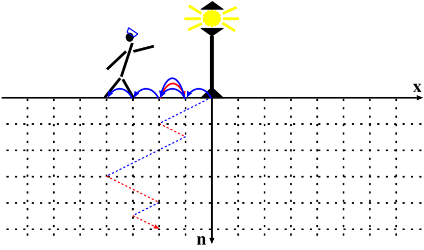
Figure 1: The “problem of the random walk” in terms of a drunken sailor at a lamppost. The space-time diagram shows an example of a trajectory for such a drunken sailor, where $n\in\mathbb{N}$ holds for discrete time and $x\in\mathbb{R}$ for the position of the sailor on a discrete lattice of spacing $s$.

Let us add a short historial note: This “problem of considerable interest” was first formulated (in three dimensions) by Karl Pearson in a letter to Nature in 1905 [Pea05]. He asked for a solution, which was provided by Lord Rayleigh referring to older work by himself [Ray05]. Pearson concluded: “The lesson of Lord Rayleigh’s solution is that in open country the most probable place to find a drunken man, who is at all capable of keeping on his feet, is somewhere near his starting point” [Pea05]. This refers to the Gaussian probability distributions for the sailor’s positions, which are obtained in a suitable scaling limit from a Gedankenexperiment with an ensemble of sailors starting from the lamppost. Fig. 2 sketches the spreading of such a diffusing distribution of sailors in time. The mathematical reason for the emerging Gaussianity of the probability distributions is nothing else than the central limit theorem [Rei65].

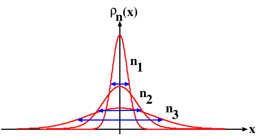
Figure 2: Probability distribution functions $\rho_{n}(x)$ to find a sailor after $n$ time steps at position $x$ on the line, calculated for an ensemble of sailors starting at the lamppost, cf. Fig. 1. Shown are three probability densities after different numbers of iteration $n_{1}<n_{2}<n_{3}$.

We may now wish to quantify the speed by which a “droplet of sailors” starting at the lamppost spreads out. This can be done by calculating the diffusion coefficient for this system. In case of one-dimensional dynamics the diffusion coefficient can be defined by the Einstein formula

$$D:=\lim_{n\to\infty}\frac{1}{2n}<x^{2}>\quad,$$ (1)

where

$$<x^{2}>:=\int dx\;x^{2}\rho_{n}(x)$$ (2)

is the variance, or second moment, of the probability distribution $\rho_{n}(x)$ at time step $n$, also called mean square displacement of the particles. This formula may be understood as follows: For our ensemble of sailors we may choose $\rho_{0}(x)=\delta(x)$ as the initial probability distribution with $\delta(x)$ denoting the (Dirac) $\delta$-function, which mimicks the situation that all sailors start at the same lamppost at $x=0$. If our system is ergodic the diffusion coefficient should be independent of the choice of the initial ensemble. The spreading of the distribution of sailors is then quantified by the growth of the mean square displacement in time. If this quantity grows linearly in time, which may not necessarily be the case but holds true if our probability distributions for the positions are Gaussian in the long-time limit [Kla07b], the magnitude of the diffusion coefficient $D$ tells us how quickly our ensemble of sailors disperses. For further details about a statistical physics description of diffusion we refer to the literature [Rei65].

In contrast to this well-known picture of diffusion as a stochastic random walk, the theory of dynamical systems makes it possible to treat diffusion as a deterministic dynamical process. Let us replace the sailor by a point particle. Instead of coin tossing, the orbit of such a particle starting at initial condition $x_{0}$ may then be generated by a chaotic dynamical system of the type as considered in the previous chapters, $x_{n+1}=F(x_{n})$. Note that defining the one-dimensional map $F(x)$ together with this equation yields the full microscopic equations of motion of the system. You may think of these equations as a caricature of Newton’s equations of motion modeling the diffusion of a single particle. Most importantly, in contrast to the drunken sailor with his memory loss after any time step here the complete memory of a particle is taken into account, that is, all steps are fully correlated. The decisive new fact that distinguishes this dynamical process from the one of a simple uncorrelated random walk is hence that $x_{n+1}$ is uniquely determined by $x_{n}$, rather than having a random distribution of $x_{n+1}$ for a given $x_{n}$. If the resulting dynamics of an ensemble of particles for given equations of motion has the property that a diffusion coefficient $D>0$ Eq. (1) exists, we speak of (normal) deterministic diffusion [Dor99, Gas98, Kla07b, Kla96b, Sch89b].

Fig. 3 shows the simple model of deterministic diffusion that we shall study in this chapter. It depicts a “chain of boxes” of chain length $L\in\mathbb{N}$, which continues periodically in both directions to infinity, and the orbit of a moving point particle. Let us first specify the map defined on the unit interval, which we may call the box map. For this we choose the map $B_{a}(x)$ introduced in our previous Example 10. We can now periodically continue this box map onto the whole real line by a lift of degree one,

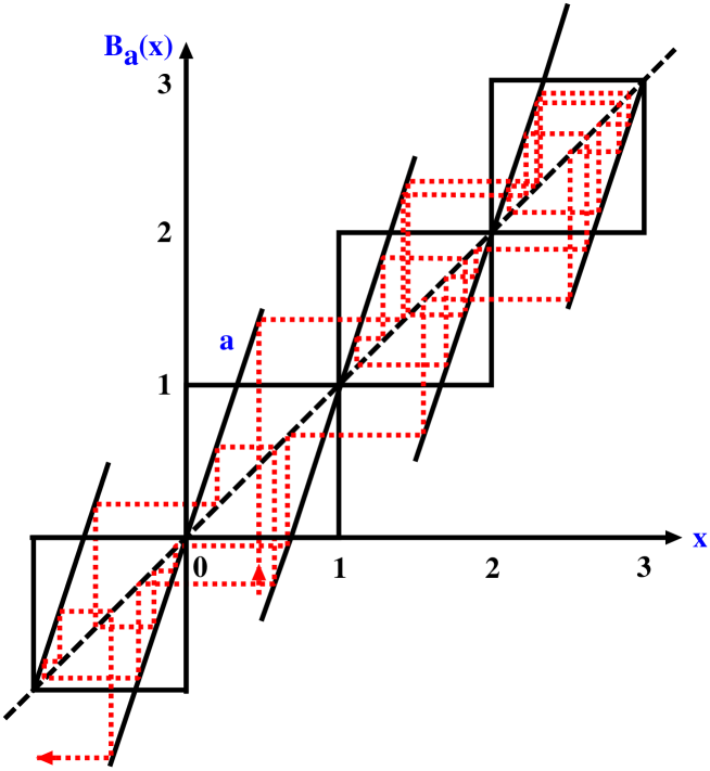
Figure 3: A simple model for deterministic diffusion. The dashed line depicts the orbit of a diffusing particle in form of a cobweb plot [All97]. The slope $a$ serves as a control parameter for the periodically continued piecewise linear map $B_{a}(x)$.

$$B_{a}(x+1)=B_{a}(x)+1\quad,$$ (3)

for which the acronym old has been introduced [Kat95]. Physically speaking, this means that $B_{a}(x)$ continued onto the real line is translational invariant with respect to integers. Note furthermore that we have chosen a box map whose graph is point symmetric with respect to the center of the box at $(x,y)=(0.5,0.5)$. This implies that the graph of the full map $B_{a}(x)$ is anti-symmetric with respect to $x=0$,

$$B_{a}(x)=-B_{a}(-x)\quad,\quad$$ (4)

so that there is no “drift” in this chain of boxes. The drift case with broken symmetry could be studied as well [Kla07b], but we exclude it here for sake of simplicity.

2 Escape rate formalism for deterministic diffusion

Before we can start with this method, let us remind ourselves about the elementary theory of diffusion in form of the diffusion equation. We then outline the basic idea underlying the escape rate formalism, which eventually yields a simple formula expressing diffusion in terms of dynamical systems quantities. Finally, we work out this approach for our deterministic model introduced before.

1 The diffusion equation

In the last section we have sketched in a nutshell what, in our setting, we mean if we speak of diffusion. This picture is made more precise by deriving an equation that exactly generates the dynamics of the probability densities displayed in Fig. 2 [Rei65]. For this purpose, let us reconsider for a moment the situation depicted in Fig. 4. There, we had a gas with an initially very high concentration of particles on the left hand side of the box. After the piston was removed, it seemed natural that the particles spread out over the right hand side of the box as well thus diffusively covering the whole box. We may thus come to the conclusion that, firstly, there will be diffusion if the density of particles in a substance is non-uniform in space. For this density of particles and by restricting ourselves to diffusion in one dimension in the following, let us write $\tilde{n}=\tilde{n}(x,t)$, which holds for the number of particles that we can find in a small line element $dx$ around the position $x$ at time step $t$ divided by the total number of particles $N$.

As a second observation, we see that diffusion occurs in the direction of decreasing particle density. This may be expressed as

$$j=:-D\frac{\partial\tilde{n}}{\partial x}\quad,$$ (5)

which according to Einstein’s formula Eq. (1) may be considered as a second definition of the diffusion coefficient $D$. Here the flux $j=j(x,t)$ denotes the number of particles passing through an area perpendicular to the direction of diffusion per time $t$. This equation is known as Fick’s first law. Finally, let us assume that no particles are created or destroyed during our diffusion process. In other words, we have conservation of the number of particles in form of

$$\frac{\partial\tilde{n}}{\partial t}+\frac{\partial j}{\partial x}=0\quad.$$ (6)

This continuity equation expresses the fact that whenever the particle density $\tilde{n}$ changes in time $t$, it must be due to a spatial change in the particle flux $j$. Combining the equation with Fick’s first law we obtain Fick’s second law,

$$\frac{\partial\tilde{n}}{\partial t}=D\frac{\partial^{2}\tilde{n}}{\partial x^{2}}\quad,$$ (7)

which is also known as the diffusion equation. Mathematicians call the process defined by this equation a Wiener process, whereas physicists rather speak of Brownian motion. If we would now solve the diffusion equation for the drunken sailor initial density $\tilde{n}(x,0)=\delta(x)$, we would obtain the precise functional form of our spreading Gaussians in Fig. 2,

$$\tilde{n}(x,t)=\frac{1}{\sqrt{4\pi Dt}}\exp{\left(-\frac{x^{2}}{4Dt}\right)}\quad.$$ (8)

Calculating the second moment of this distribution according to Eq. (2) would lead us to recover Einstein’s definition of the diffusion coefficient Eq. (1). Therefore, both this definition and the one provided by Fick’s first law are consistent with each other.

2 Basic idea of the escape rate formalism

We are now fully prepared for establishing an interesting link between dynamical systems theory and statistical mechanics. We start with a brief outline of the concept of this theory, which is called the escape rate formalism, pioneered by Gaspard and others [Gas90, Gas98, Dor99]. It consists of three steps:

Step 1: Solve the one-dimensional diffusion equation Eq. (7) derived above for absorbing boundary conditions. That is, we consider now some type of open system similar to what we have studied in the previous chapter. We may thus expect that the total number of particles $N(t):=\int dx\>\tilde{n}(x,t)$ within the system decreases exponentially as time evolves according to the law expressed by Eq. (42), that is,

$$N(t)=N(0)e^{-\gamma_{de}t}\quad.$$ (9)

It will turn out that the escape rate $\gamma_{de}$ defined by the diffusion equation with absorbing boundaries is a function of the system size $L$ and of the diffusion coefficient $D$.

Step 2: Solve the Frobenius-Perron equation

$$\rho_{n+1}(x)=\int dy\>\rho_{n}(y)\>\delta(x-F(y))\quad,$$ (10)

which represents the continuity equation for the probability density $\rho_{n}(x)$ of the map $F(x)$ [Ott93, Bec93, Dor99], for the very same absorbing boundary conditions as in Step 1. Let us assume that the dynamical system under consideration is normal diffusive, that is, that a diffusion coefficient $D>0$ exists. We may then expect a decrease in the number of particles that is completely analogous to what we have obtained from the diffusion equation. That is, if we define as before $N_{n}:=\int dx\>\rho_{n}(x)$ as the total number of particles within the system at discrete time step $n$, in case of normal diffusion we should obtain

$$N_{n}=N_{0}e^{-\gamma_{FP}n}\quad.$$ (11)

However, in contrast to Step 1 here the escape rate $\gamma_{FP}$ should be fully determined by the dynamical system that we are considering. In fact, we have already seen before that for open systems the escape rate can be expressed exactly as the difference between the positive Ljapunov exponent and the KS-entropy on the fractal repeller, cf. the escape rate formula Eq. (53).

Step 3: If the functional forms of the particle density $\tilde{n}(x,t)$ of the diffusion equation and of the probability density $\rho_{n}(x)$ of the map’s Frobenius-Perron equation match in the limit of system size and time going to infinity — which is what one has to show —, the escape rates $\gamma_{de}$ obtained from the diffusion equation and $\gamma_{FP}$ calculated from the Frobenius-Perron equation should be equal,

$$\gamma_{de}=\gamma_{FP}\quad,$$ (12)

providing a fundamental link between the statistical physical theory of diffusion and dynamical systems theory. Since $\gamma_{de}$ is a function of the diffusion coefficient $D$, and knowing that $\gamma_{FP}$ is a function of dynamical systems quantities, we should then be able to express $D$ exactly in terms of these dynamical systems quantifiers. We will now illustrate how this method works by applying it to our simple deterministic diffusive model introduced above.

3 The escape rate formalism worked out for a simple map

Let us consider the map $B_{a}(x)$ lifted onto the whole real line for the specific parameter value $a=4$, see Fig. 4. With $L$ we denote the chain length. Proceeding along the above lines, let us start with

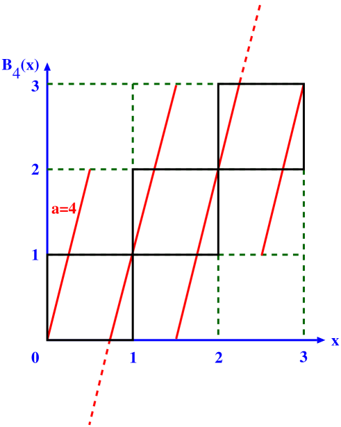
Figure 4: Our previous map $B_{a}(x)$ periodically continued onto the whole real line for the specific parameter value $a=4$. The example shown depicts a chain of length $L=3$. The dashed quadratic grid indicates a Markov partition for this map.

Step 1: Solve the one-dimensional diffusion equation Eq. (7) for the absorbing boundary conditions

$$\tilde{n}(0,t)=\tilde{n}(L,t)=0\quad,$$ (13)

which models the situation that particles escape precisely at the boundaries of our one-dimensional domain. A straightforward calculation yields

$$\tilde{n}(x,t)=\sum_{m=1}^{\infty}b_{m}\exp\left(-\left(\frac{m\pi}{L}\right)^{2}Dt\right)\sin\left(\frac{m\pi}{L}x\right)$$ (14)

with $b_{m}$ denoting the Fourier coefficients.

Step 2: Solve the Frobenius-Perron equation Eq. (10) for the same absorbing boundary conditions,

$$\rho_{n}(0)=\rho_{n}(L)=0\quad.$$ (15)

In order to do so, we first need to introduce a concept called Markov partition for our map $B_{4}(x)$:

Definition 11

Markov partition, verbally [Bec93, Kla07a]

For one-dimensional maps acting on compact intervals a partition is called Markov if parts of the partition get mapped again onto parts of the partition, or onto unions of parts of the partition.

Example 13

The dashed quadratic grid in Fig. 4 defines a Markov partition for the lifted map $B_{4}(x)$.

Of course there also exists a precise formal definition of Markov partitions, however, here we do not elaborate on these technical details [Kla07a]. Having a Markov partition at hand enables us to rewrite the Frobenius-Perron equation in form of a matrix equation, where a Frobenius-Perron matrix operator acts onto probability density vectors defined with respect to this special partitioning. In order to see this, consider an initial density of points that covers, e.g., the interval in the second box of Fig. 4 uniformly. By applying the map onto this density, one observes that points of this interval get mapped two-fold onto the interval in the second box again, but that there is also escape from this box which uniformly covers the third and the first box intervals, respectively. This mechanism applies to any box in our chain of boxes, modified only by the absorbing boundary conditions at the ends of the chain of length $L$. Taking into account the stretching of the density by the slope $a=4$ at each iteration, this suggests that the Frobenius-Perron equation Eq. (10) can be rewritten as

$$\mbox{\boldmath$\rho$}_{n+1}=\frac{1}{4}\,T(4)\,\mbox{\boldmath$\rho$}_{n}\quad,$$ (16)

where the $L$ x $L$-transition matrix $T(4)$ must read

$$T(4)=\left(\begin{array}[]{cccccccc}2&1&0&0&\cdots&0&0&0\\ 1&2&1&0&0&\cdots&0&0\\ 0&1&2&1&0&0&\cdots&0\\ \vdots&&&\vdots&\vdots&&&\vdots\\ 0&\cdots&0&0&1&2&1&0\\ 0&0&\cdots&0&0&1&2&1\\ 0&0&0&\cdots&0&0&1&2\\ \end{array}\right)\quad.$$ (17)

Note that in any row and in any column we have three non-zero matrix elements except in the very first and the very last rows and columns, which reflect the absorbing boundary conditions. In Eq.(16) this transition matrix $T(4)$ is applied to a column vector $\mbox{\boldmath$\rho$}_{n}$ corresponding to the probability density $\rho_{n}(x)$, which can be written as

$$\mbox{\boldmath$\rho$}_{n}=|\rho_{n}(x)>:=(\rho_{n}^{1},\rho_{n}^{2},\ldots,\rho_{n}^{k},\ldots,\rho_{n}^{L})^{*}\quad,$$ (18)

where “$*$” denotes the transpose and $\rho_{n}^{k}$ represents the component of the probability density in the $k$th box, $\rho_{n}(x)=\rho_{n}^{k}\;,\;k-1<x\leq k\;,\;k=1,\ldots,L\;$, $\rho_{n}^{k}$ being constant on each part of the partition. We see that this transition matrix is symmetric, hence it can be diagonalized by spectral decomposition. Solving the eigenvalue problem

$$T(4)\,|\phi_{m}(x)>=\chi_{m}(4)\,|\phi_{m}(x)>\quad,$$ (19)

where $\chi_{m}(4)$ and $|\phi_{m}(x)>$ are the eigenvalues and eigenvectors of $T(4)$, respectively, one obtains

$$|\rho_{n}(x)> = \frac{1}{4}\sum_{m=1}^{L}\chi_{m}(4)\,|\phi_{m}(x)><\phi_{m}(x)|\rho_{n-1}(x)>$$ (20)

$$= \sum_{m=1}^{L}\exp\left(-n\ln\frac{4}{\chi_{m}(4)}\right)\,|\phi_{m}(x)><\phi_{m}(x)|\rho_{0}(x)>\quad,$$

where $|\rho_{0}(x)>$ is the initial probability density vector. Note that the choice of initial probability densities is restricted by this method to functions that can be written in the vector form of Eq.(18). It remains to solve the eigenvalue problem Eq. (19) [Kla95, Kla99]. The eigenvalue equation for the single components of the matrix $T(4)$ reads

$$\phi_{m}^{k}+2\phi_{m}^{k+1}+\phi_{m}^{k+2}=\chi_{m}\phi_{m}^{k+1}\quad,\quad 0\leq k\leq L-1\quad,$$ (21)

supplemented by the absorbing boundary conditions

$$\phi_{m}^{0}=\phi_{m}^{L+1}=0\quad.$$ (22)

This equation is of the form of a discretized ordinary differential equation of degree two, hence we make the ansatz

$$\phi_{m}^{k}=a\cos(k\theta)+b\sin(k\theta)\quad,\quad 0\leq k\leq L+1\quad.$$ (23)

The two boundary conditions lead to

$$a=0\quad\mbox{and}\quad\sin((L+1)\theta)=0$$ (24)

yielding

$$\theta_{m}=\frac{m\pi}{L+1}\quad,\quad 1\leq m\leq L\quad.$$ (25)

The eigenvectors are then determined by

$$\phi_{m}^{k}=b\sin(k\theta_{m})\quad.$$ (26)

Combining this equation with Eq. (21) yields as the eigenvalues

$$\chi_{m}=2+2\cos\theta_{m}\quad.$$ (27)

Step 3: Putting all details together, it remains to match the solution of the diffusion equation to the one of the Frobenius-Perron equation: In the limit of time $t$ and system size $L$ to infinity, the density $\tilde{n}(x,t)$ Eq. (14) of the diffusion equation reduces to the largest eigenmode,

$$\tilde{n}(x,t)\simeq\exp\left(-\gamma_{de}t\right)B\sin\left(\frac{\pi}{L}x\right)\quad,$$ (28)

where

$$\gamma_{de}:=\left(\frac{\pi}{L}\right)^{2}D$$ (29)

defines the escape rate as determined by the diffusion equation. Analogously, for discrete time $n$ and chain length $L$ to infinity we obtain for the probability density of the Frobenius-Perron equation, Eq.(20) with Eq.(26),

$$\rho_{n}(x) \simeq \exp\left(-\gamma_{FP}n\right)\tilde{B}\sin\left(\frac{\pi}{L+1}k\right)\quad,$$ (30)

$$k=0,\ldots,L+1\quad,\quad k-1<x\leq k$$

with an escape rate of this dynamical system given by

$$\gamma_{FP}=\ln\frac{4}{2+2\cos(\pi/(L+1))}\quad,$$ (31)

which is determined by the largest eigenvalue $\chi_{1}$ of the matrix $T(4)$, see Eq.(20) with Eq.(27). We can now see that the functional forms of the eigenmodes of Eqs.(28) and (30) match precisely. This allows us to match Eqs. (29) and (31) leading to

$$D(4)=\left(\frac{L}{\pi}\right)^{2}\gamma_{FP}\quad.$$ (32)

Using the right hand side of Eq. (31) and expanding it for $L\to\infty$, this formula enables us to calculate the diffusion coefficient $D(4)$ to

$$D(4)=\left(\frac{L}{\pi}\right)^{2}\gamma_{FP}=\frac{1}{4}\frac{L^{2}}{(L+1)^{2}}+{\cal O}(L^{-4})\;\to\;\frac{1}{4}\quad(L\rightarrow\infty)\quad.$$ (33)

Thus we have developed a method by which we can exactly calculate the deterministic diffusion coefficient of a simple chaotic dynamical system. However, more importantly, instead of using the explicit expression for $\gamma_{FP}$ given by Eq. (31), let us remind ourselves of the escape rate formula Eq. (53) for $\gamma_{FP}$,

$$\gamma_{FP}=\gamma({\cal C}_{B_{4}})=\lambda({\cal C}_{B_{4}})-h_{KS}({\cal C}_{B_{4}})\quad,$$ (34)

which more geneally expresses this escape rate in terms of dynamical systems quantities. Combining this equation with the above equation Eq. (32) leads to our final result, the escape rate formula for deterministic diffusion [Gas90, Gas98]

$$D(4)=\lim_{L\to\infty}\left(\frac{L}{\pi}\right)^{2}\left[\lambda({\cal C}_{B_{4}})-h_{KS}({\cal C}_{B_{4}})\right]\quad.$$ (35)

We have thus established a fundamental link between quantities assessing the chaotic properties of dynamical systems and the statistical physical property of diffusion.

Remark 3

1. Above we have only considered the special case of the control parameter $a=4$. Along the same lines, the diffusion coefficient can be calculated for other parameter values of the map $B_{a}(x)$. Surprisingly, the parameter-dependent diffusion coefficient of this map turns out to be a fractal function of the control parameter [Kla95, Kla96b, Kla99]. This result is believed to hold for a wide class of dynamical systems [Kla07b].

2. The escape rate formula for diffusion does not only hold for simple one-dimensional maps but can be generalized to higher-dimensional time-discrete as well as time-continuous dynamical systems [Gas98, Dor99].

3. This approach can also be generalized to establish relations between chaos and transport for other transport coefficients such as viscosity, heat conduction and chemical reaction rates [Gas98].

4. This is not the only approach connecting transport properties with dynamical systems quantities. In recent research it was found that there exist at least two other ways to establish relations that are different but of a very similar nature; see [Kla07b] for further details.

Chapter 3 Anomalous diffusion

In the last section we have explored diffusion for a simple piecewise linear map. One may now wonder what type of diffusive behavior is encountered if we consider more complicated models. Straightforward generalizations are nonlinear maps generating intermittency. In Section 1 we briefly illustrate the phenomenon of intermittency and introduce the concept of anomalous diffusion. We then give an outline of continuous time random walk theory, which is a powerful tool of stochastic theory that models anomalous diffusion. By using this method we derive a fractional diffusion equation, which generalizes Fick’s second law that we have encountered before to this type of anomalous diffusion.

After having restricted ourselves to rather abstract but mostly solvable models, we conclude our review by discussing an experiment which gives evidence for the existence of anomalous diffusion in a fundamental biological process. Section 2 first motivates the problem of cell migration. We then present experimental results for two different cell types and explain them by suggesting a model reproducing the observed anomalous dynamics of cell migration.

Section 1 particularly draws on Refs. [Kor05, Kor07], see also Section 6.2 of [Kla07b], Section 2 is based on Ref. [Die08]. For more general introductions to the very active field of anomalous transport see, e.g., Refs. [Shl93, Kla96a, Met00, Kla08].

1 Anomalous diffusion in intermittent maps

1 What is anomalous diffusion?

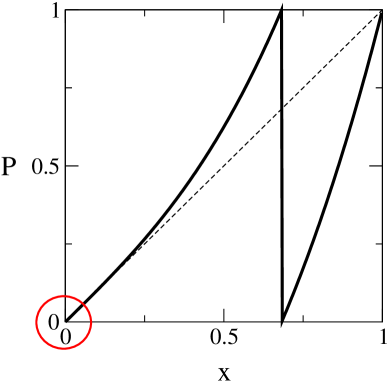
Figure 1: The Pomeau-Manneville map Eq. (1) for $a=1$ and $z=3$. Note that there is a marginal fixed point at $x=0$ leading to the intermittent behavior depicted in Fig. 2.

Let us consider a simple variant of our previous piecewise linear model, which is the Pomeau-Manneville map [Pom80]

$$P_{a,z}(x)=x+ax^{z}\;\;\mbox{mod}1\quad,$$ (1)

see Fig. 1, where as usual the dynamics is defined by $x_{n+1}=P_{a,z}(x_{n})$. This map has two control parameters, $a\geq 1$ and the exponent of nonlinearity $z\geq 1$. For $a=1$ and $z=1$ this map just reduces to our familiar Bernoulli shift Eq. (3), however, for $z>1$ it provides a nontrivial nonlinear generalization of it. The nontriviality is due to the fact that in this case the stability of the fixed point at $x=0$ becomes marginal (sometimes also called indifferent, or neutral), $P^{\prime}_{a,z}(0)=1$. Since the map is smooth around $x=0$, the dynamics resulting from the left branch of the map is determined by the stability of this fixed point, whereas the right branch is just of Bernoulli shift-type yielding ordinary chaotic dynamics. There is thus a competition in the dynamics between these two different branches as illustrated by Fig. 2: One can observe that long periodic laminar phases determined by the marginal fixed point around $x=0$ are interrupted by chaotic bursts reflecting the “Bernoulli shift-like part” of the map with slope $a>1$ around $x=1$. This phenomenology is the hallmark of what is called intermittency [Sch89b, Ott93].

Figure 2: Phenomenology of intermittency in the Pomeau-Manneville map Fig. 1: The plot shows the time series of position $x_{n}$ versus discrete time step $n$ for an orbit generated by the map Eq. (1), which starts at a typical initial condition $x_{0}$.

Following Section 1 it is now straightforward to define a spatially extended version of the Pomeau-Manneville map: For this purpose we just continue $P_{a,z}(x)=x+ax^{z}\;,\;0\leq x<\frac{1}{2}$ in Eq. (1) onto the real line by the translation $P_{a,z}(x+1)=P_{a,z}(x)+1$, see Eq. (3), under reflection symmetry $P_{a,z}(-x)=-P_{a,z}(x)$, see Eq. (4). The resulting model  [Gei84, Zum93] is displayed in Fig. 3. As before, we may now be interested in the type of deterministic diffusion generated by this model. Surprisingly, by calculating the mean square displacement Eq. (2) either analytically or from computer simulations one finds that for $z>2$

Figure 3: The Pomeau-Manneville map Fig. 1, Eq. (1), lifted symmetrically onto the whole real line such that it generates subdiffusion.

$$\left<x^{2}\right>\sim\>n^{\alpha}\quad,\quad\alpha<1\quad(n\to\infty)\quad.$$ (2)

This implies that the diffusion coefficient $D:=\lim_{n\to\infty}<x^{2}>/(2n)$ as defined by Eq. (1) is simply zero, despite the fact that particles can go anywhere on the real line as shown in Fig. 3. We thus encounter a novel type of diffusive behavior classified by the following definition:

Definition 12

anomalous diffusion [Met00, Kla08]

If the exponent $\alpha$ in the temporal spreading of the mean square displacement Eq. (2) of an ensemble of particles is not equal to one, one speaks of anomalous diffusion. If $\alpha<1$ one says that there is subdiffusion, for $\alpha>1$ there is superdiffusion, and in case of $\alpha=1$ one refers to normal diffusion. The constant

$$K:=\lim_{n\to\infty}\frac{<x^{2}>}{n^{\alpha}}\quad,$$ (3)

where in case of normal diffusion $K=2D$, is called the generalized diffusion coefficient.

We will now discuss how $K$ behaves as a function of $a$ for our new model and then show how the exponent $\alpha$ and, in an approximation, $K$, can be calculated analytically. This can be achieved by means of continuous time random walk (CTRW) theory, which provides a generalization of the drunken sailor’s model introduced in Section 1 to anomalous dynamics.

2 Continuous time random walk theory

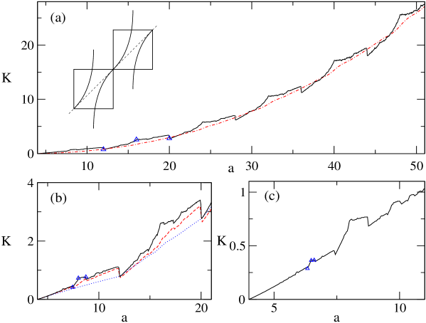
Figure 4: The generalized diffusion coefficient $K$ Eq. (3) as a function of $a$ for $z=3$. The curve in (a) consists of $1200$ points, the dashed-dotted line displays the CTRW result $K_{1}$, Eqs. (14), (16). (b) (600 points) and (c) (200 points) show magnifications of (a) close to the onset of diffusion. The dotted line in (b) is the CTRW approximation $K_{2}$, Eqs. (15), (16), the dashed line represents yet another semi-analytical approximation as detailed in Refs. [Kor05, Kor07]. The triangles mark a specific structure appearing on finer and finer scales. The inset in (a) depicts again the model Eq. (1).

Let us first study the diffusive behavior of the map displayed in Fig. 3 by computer simulations. As we will explain in detail below, stochastic theory predicts that for this map it is

$$\alpha=\begin{cases}1,&1\leq z<2\cr\frac{1}{z-1},&2\leq z\end{cases}$$ (4)

[Gei84, Zum93]. For all values of the second control parameter $a$ we indeed find excellent agreement between these analytical solutions and the results for $\alpha$ obtained from simulations. Consequently, $\alpha$ is determined by Eq. (4) in the following for extracting the generalized diffusion coefficient $K$ Eq. (3) from simulations.

While in Chapter 2 we have only discussed diffusion for a specific choice of the control parameter, we now study the behavior of $K$ as a function of $a$ for fixed $z$. Computer simulation results are displayed in Fig. 4. Magnifications of part (a) shown in parts (b) and (c) reveal self similar-like irregularities indicating a fractal parameter dependence of $K=K(a)$. This fractality is highlighted by the sub-structure identified through triangles, which is repeated on finer and finer scales. The parameter values for these symbols correspond to specific series of Markov partitions. Details are explained in Refs. [Kla95, Kla96b, Kla99] for parameter-dependent diffusion in the piecewise linear one-dimensional maps studied in Chapter 2, which exhibits quite analogous structures. Over the past few years such fractal transport coefficients have been revealed for a number of different models. They are conjectured to be a typical phenomenon if the dynamical system is deterministic, low-dimensional and spatially periodic. Their origin can be understood in terms of microscopic long-range dynamical correlations that, due to topological instabilities of dynamical systems, change in a complicated manner under parameter variation. Although it has been argued that such highly irregular behavior of transport coefficients should also occur in physically realistic systems, it has not yet clearly been observed in experiments; see Ref. [Kla07b] for a review of this line of research.

Instead of elaborating on the fractality in detail, here we reproduce the course functional form of $K(a)$ by using stochastic CTRW theory. Pioneered by Montroll, Weiss and Scher [Mon65, Mon73, Sch75], it yields perhaps the most fundamental theoretical approach to explain anomalous diffusion [Bou90, Wei94, Ebe05]. In further groundbreaking works by Geisel et al. and Klafter et al., this method was then adapted to sub- and superdiffusive deterministic maps [Gei84, Gei85, Shl85, Zum93]

The basic assumption of the approach is that diffusion can be decomposed into two stochastic processes characterized by waiting times and jumps, respectively. Thus one has two sequences of independent identically distributed random variables, namely a sequence of positive random waiting times $T_{1},T_{2},T_{3},\ldots$ with probability density function $w(t)$ and a sequence of random jumps $\zeta_{1},\zeta_{2},\zeta_{3},\ldots$ with a probability density function $\lambda(x)$. For example, if a particle starts at point $x=0$ at time $t_{0}=0$ and makes a jump of length $\zeta_{n}$ at time $t_{n}=T_{1}+T_{2}+...+T_{n}$, its position is $x=0$ for $0\leq t<T_{1}=t_{1}$ and $x=\zeta_{1}+\zeta_{2}+...+\zeta_{n}$ for $t_{n}\leq t<t_{n+1}$. The probability that at least one jump is performed within the time interval $[0,t)$ is then $\int_{0}^{t}dt^{\prime}w(t^{\prime})$ while the probability for no jump during this time interval reads $\Psi(t)=1-\int_{0}^{t}dt^{\prime}w(t^{\prime})$. The master equation for the probability density function $P(x,t)$ to find a particle at position $x$ and time $t$ is then

$$P(x,t)=\int_{-\infty}^{\infty}dx^{\prime}\lambda(x-x^{\prime})\int_{0}^{t}dt^{\prime}\;w(t-t^{\prime})\;P(x^{\prime},t^{\prime})+\Psi(t)\delta(x)\quad.$$ (5)

It has the following probabilistic meaning: The probability density function to find a particle at position $x$ at time $t$ is equal to the probability density function to find it at point $x^{\prime}$ at some previous time $t^{\prime}$ multiplied with the transition probability to get from $(x^{\prime},t^{\prime})$ to $(x,t)$ integrated over all possible values of $x^{\prime}$ and $t^{\prime}$. The second term accounts for the probability of remaining at the initial position $x=0$. The most convenient representation of this equation is obtained in terms of the Fourier-Laplace transform of the probability density function,

$$\hat{\tilde{P}}(k,s)=\int_{-\infty}^{\infty}dx\;e^{ikx}\int_{0}^{\infty}dt\;e^{-st}P(x,t)\quad,$$ (6)

where the hat stands for the Fourier transform and the tilde for the Laplace transform. Respectively, this function obeys the Fourier-Laplace transform of Eq. (5), which is called the Montroll-Weiss equation [Mon65, Mon73, Sch75],

$$\hat{\tilde{P}}(k,s)=\frac{1-\tilde{w}(s)}{s}\frac{1}{1-\hat{\lambda}(k)\tilde{w}(s)}\quad.$$ (7)

The Laplace transform of the mean square displacement can be readily obtained by differentiating the Fourier-Laplace transform of the probability density function,

$$\tilde{\left<x^{2}(s)\right>}=\int_{-\infty}^{\infty}dx\;x^{2}\tilde{P}(x,s)=\left.-\frac{\partial^{2}\hat{\tilde{P}}(k,s)}{\partial k^{2}}\right|_{k=0}\quad.$$ (8)

In order to calculate the mean square displacement within this theory, it thus suffices to know $\lambda(x)$ and $w(t)$ generating the stochastic process. For one-dimensional maps of the type of Eq. (1), exploiting the symmetry of the map the waiting time distribution can be calculated from the approximation

$$x_{n+1}-x_{n}\simeq\frac{dx_{t}}{dt}=ax_{t}^{z},\;\;x\ll 1\quad,$$ (9)

where we have introduced the continuous time $t\geq 0$. This equation can easily be solved for $x_{t}$ with respect to an initial condition $x_{0}$. Now one needs to define when a particle makes a “jump”, as will be discussed below. By inverting the solution for $x_{t}$, one can then calculate the time $t$ a particle has to wait before it makes a jump as a function of the initial condition $x_{0}$. This information determines the relation between the waiting time probability density $w(t)$ and the as yet unknown probability density of injection points,

$$w(t)\simeq P_{in}(x_{0})\left|\frac{dx_{0}}{dt}\right|\quad.$$ (10)

Making the assumption that the probability density of injection points is uniform, $P_{in}\simeq 1$, the waiting time probability density is straightforwardly calculated from the knowledge of $t(x_{0})$. The second ingredient that is needed for the CTRW approach is the jump probability density. Standard CTRW theory takes jumps between neighbouring cells only into account leading to the ansatz [Gei84, Zum93]

$$\lambda(x)=\delta(|x|-1)\quad.$$ (11)

It turns out that a correct application of this theory to our results for $K(a)$ requires a modification of the standard theory at three points: Firstly, the waiting time probability density function must be calculated according to the grid of elementary cells indicated in Fig. 4 [Kla96b, Kla97] yielding

$$w(t)=a\left(1+a(z-1)t\right)^{-\frac{z}{z-1}}\quad.$$ (12)

However, this probability density function also accounts for attempted jumps to another cell, since after a step the particle may stay in the same cell with a probability of $(1-p)$. The latter quantity is roughly determined by the size of the escape region $p=(1-2x_{c})$ with $x_{c}$ as a solution of the equation $x_{c}+ax^{z}_{c}=1$. We thus model this fact, secondly, by a jump length distribution in the form of

$$\lambda(x)=\frac{p}{2}\delta(\left|x\right|-l)+(1-p)\delta(x)\>.$$ (13)

Thirdly, we introduce two definitions of a typical jump length $l_{i}\>,i\in\{1,2\}$.

$$l_{1}=\left\{|M_{a,z}(x)-x|\right\}\>$$ (14)

corresponds to the actual mean displacement while

$$l_{2}=\left\{|[M_{a,z}(x)]|\right\}\>$$ (15)

gives the coarse-grained displacement in units of elementary cells, as it is often assumed in CTRW approaches. In these definitions $\left\{\ldots\right\}$ denotes both a time and ensemble average over particles leaving a box. Working out the modified CTRW approximation sketched above by taking these three changes into account we obtain for the generalized diffusion coefficient

$$K_{i}=pl_{i}^{2}\left\{\begin{array}[]{l@{\quad,\quad}l}a^{\gamma}\sin(\pi\gamma)/\pi\gamma^{1+\gamma}&0<\gamma<1\\ a(1-1/\gamma)&1\leq\gamma<\infty\end{array}\right.\quad,$$ (16)

where $\gamma:=1/(z-1)$, which for $z\geq 2$ is identical with $\alpha$ defined in Eq. (4). Fig. 4 (a) shows that $K_{1}$ well describes the coarse functional form of $K$ for large $a$. $K_{2}$ is depicted in Fig. 4 (b) by the dotted line and is asymptotically exact in the limit of very small $a$. Hence, the generalized diffusion coefficient exhibits a dynamical crossover between two different coarse grained functional forms for small and large $a$, respectively. An analogous crossover has been reported earlier for normal diffusion [Kla96b, Kla97] and was also found in other models [Kla07b].

Let us finally focus on the generalized diffusion coefficient at $a=12,20,28,...$, which correspond to integer values of the height $h=[M_{a,z}(1/2)]$ of the map. Simulations reproduce, within numerical accuracy, the results for $K_{2}$ by indicating that $K$ is discontinuous at these parameter values. Due to the self similar-like structure of the generalized diffusion coefficient it was thus conjectured that the precise $K$ of our model exhibits infinitely many discontinuities on fine scales as a function of $a$, which is at variance with the continuity of the CTRW approximation [Kor05, Kor07]. This highlights again that CTRW theory gives only an approximate solution for the generalized diffusion coefficient of this model.

3 A fractional diffusion equation

We now turn to the probability density functions (PDFs) generated by the map Eq. (1). As we will show now, CTRW theory not only predicts the power $\gamma$ correctly but also the form of the coarse grained PDF $P(x,t)$ of displacements. Correspondingly the anomalous diffusion process generated by our model is not described by an ordinary diffusion equation but by a generalization of it. Starting from the Montroll-Weiss equation and making use of the expressions for the jump and waiting time PDFs Eqs. (11), (12), we rewrite Eq. (7) in the long-time and -space asymptotic form

$$s^{\gamma}\hat{\tilde{P}}-s^{\gamma-1}=-\frac{pl_{i}^{2}}{2cb^{\gamma}}k^{2}\hat{\tilde{P}}$$ (17)

with $c=\Gamma(1-\gamma)$ and $b=\gamma/a$. For the initial condition $P(x,0)=\delta(x)$ of the PDF we have $\hat{P}(k,0)=1$. Interestingly, the left hand side of this equation corresponds to the definition of the Caputo fractional derivative of a function $G$,

$$\frac{\partial^{\gamma}G}{\partial t^{\gamma}}:=\frac{1}{\Gamma(1-\gamma)}\;\int_{0}^{t}dt^{{}^{\prime}}(t-t^{{}^{\prime}})^{-\gamma}\frac{\partial G}{\partial t^{{}^{\prime}}}\quad,$$ (18)

in Laplace space [Pod99, Mai97],

$$\int_{0}^{\infty}dt\;e^{-st}\frac{\partial^{\gamma}G}{\partial t^{\gamma}}=s^{\gamma}\tilde{G}(s)-s^{\gamma-1}G(0)\quad.$$ (19)

Thus, fractional derivatives come naturally into play as a suitable mathematical formalism whenever there are power law memory kernels in space and/or time generating anomalous dynamics; see, e.g., Refs. [Sok02, Met00] for short introductions to fractional derivatives and Ref. [Pod99] for a detailed exposition. Turning back now to real space, we thus arrive at the time-fractional diffusion equation

$$\frac{\partial^{\gamma}P(x,t)}{\partial t^{\gamma}}=D\;\frac{\partial^{2}P}{\partial x^{2}}$$ (20)

with $D=K\Gamma(1+\gamma)/2$, $0<\gamma<1$, which is an example of a fractional diffusion equation generating subdiffusion. For $\gamma=1$ we recover the ordinary diffusion equation. The solution of Eq. (20) can be expressed in terms of an M-function of Wright type [Mai97] and reads

$$P(x,t)=\frac{1}{2\sqrt{D}t^{\gamma/2}}M\left(\xi,\frac{\gamma}{2}\right)\quad.$$ (21)

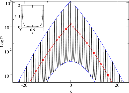
Figure 5: Comparison of the probability density obtained from simulations of the map Eq. (1) (oscillatory structure) with the analytical solution Eq. (21) of the fractional diffusion equation Eq. (20) (continuous line in the middle) for $z=3$ and $a=8$. The probability density was computed from $10^{7}$ particles after $n=10^{3}$ iterations. For the generalized diffusion coefficient in Eq. (21) the simulation result was used. The crosses (x) represent the numerical results coarse grained over unit intervals. The upper and the lower curves correspond to fits with a stretched exponential and a Gaussian distribution, respectively. The inset depicts the probability density function for the map on the unit interval with periodic boundaries.

Fig. 5 demonstrates an excellent agreement between the analytical solution Eq. (21) and the PDF obtained from simulations of the map Eq. (1) if the PDF is coarse grained over unit intervals. However, it also shows that the coarse graining eliminates a periodic fine structure that is not captured by Eq. (21). This fine structure derives from the “microscopic” PDF of an elementary cell (with periodic boundaries) as represented in the inset of Fig. 5 [Kla96b]. The singularities are due to the marginal fixed points of the map, where particles are trapped for long times. Remarkably, that way the microscopic origin of the intermittent dynamics is reflected in the shape of the PDF on the whole real line: From Fig. 5 it is seen that the oscillations in the PDF are bounded by two functions, the upper curve being of a stretched exponential type while the lower is Gaussian. These two envelopes correspond to the laminar and chaotic parts of the motion, respectively.

2 Anomalous diffusion of migrating biological cells

1 Cell migration

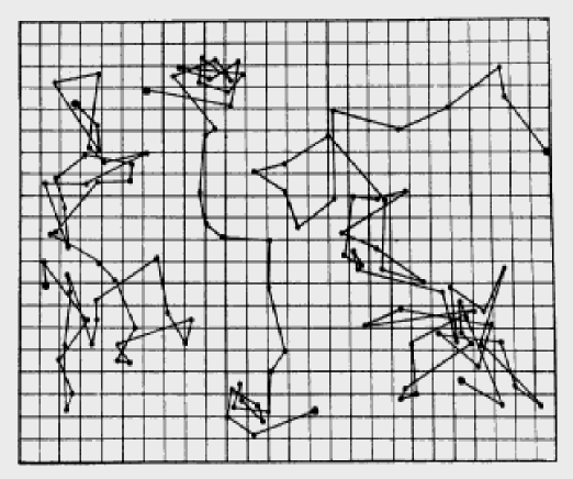
Figure 6: Trajectories of three colloidal particles of radius $0.53\mu$m whose positions have been measured experimentally every 30 seconds. Single points are joined by straight lines [Per09].

We start this final section with results from a famous experiment. Fig. 6 shows the trajectories of three colloidal particles immersed in a fluid. Their motion looks highly irregular thus reminding us of the trajectory of the drunken sailor’s problem displayed in Fig. 1. As we discussed in Chapter 2, dynamics which can be characterized by a normal diffusion coefficient is called Brownian motion. It was Einstein’s achievement to understand the diffusion of molecules in a fluid in terms of such microscopic dynamics [Ein05]. His theory actually motivated Perrin to conduct his experiment by which Einstein’s theory was confirmed [Per09].

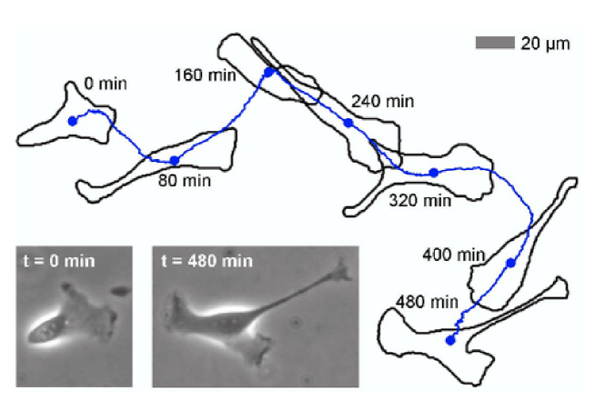
Figure 7: Overlay of a biological cell migrating on a substrate. The cell frequently changes its shape and direction during migration, as is shown by several cell contours extracted during the migration process. The inset displays phase contrast images of the cell at the beginning and to the end of its migration process [Die08].

Fig. 7 now shows the trajectory of a very different type of process. Displayed is the path of a single biological cell crawling on a substrate [Die08]. Nearly all cells in the human body are mobile at a given time during their life cycle. Embryogenesis, wound-healing, immune defense and the formation of tumor metastases are well known phenomena that rely on cell migration. If one compares the cell trajectory with the one of the Brownian particles depicted in Fig. 6, one may find it hard to see a fundamental difference. On the other hand, according to Einstein’s theory a Brownian particle is passively driven by collisions from the surrounding particles, whereas biological cells move actively by themselves converting chemical into kinetic energy. This raises the question whether the dynamics of cell migration can really be understood in terms of Brownian motion [Dun87, Sto91] or whether more advanced concepts of dynamical modeling have to be applied [Har94, Upa01].

2 Experimental results

The cell migration experiments that we now discuss have been performed on two transformed renal epithelial Madin– Darby canine kidney (MDCK-F) cell strains: wild-type ($NHE^{+}$) and NHE-deficient ($NHE^{-}$) cells. The cell diameter is typically 20-50$\mu$m and the mean velocity of the cells about $1\mu$m/min. The lamellipodial dynamics, which denotes the fluctuations of the cell body surrounding the cell nucleus, called cytoskeleton, that drives the cell migration, is of the order of seconds. Thirteen cells were observed for up to 1000 minutes. Sequences of microscopic phase contrast images were taken and segmented to obtain the cell boundaries shown in Fig. 7; see Ref. [Die08] for full details of the experiment.

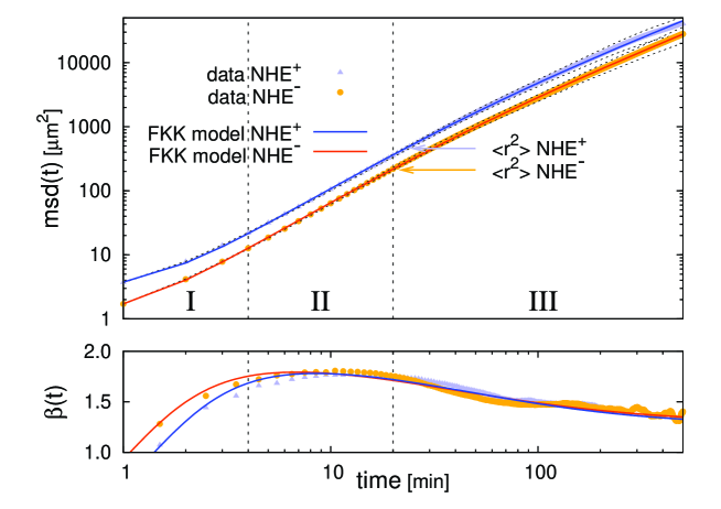
Figure 8: Upper part: Double-logarithmic plot of the mean square displacement (msd) as a function of time. Experimental data points for both cell types are shown by symbols. Different time scales are marked as phases I, II and III as discussed in the text. The solid lines represent fits to the msd from the solution of our model, see Eq. (28). All parameter values of the model are given in [Die08]. The dashed lines indicate the uncertainties of the msd values according to Bayes data analysis. Lower part: Logarithmic derivative $\beta(t)$ of the msd for both cell types.

As we have learned in Chapter 2, Brownian motion is characterized by a mean square displacement (msd) proportional to $t$ in the limit of long time designating normal diffusion. Fig. 8 shows that both types of cells behave differently: First of all, MDCK-F $NHE^{-}$ cells move less efficiently than $NHE^{+}$ cells resulting in a reduced msd for all times. As is displayed in the upper part of this figure, the msd of both cell types exhibits a crossover between three different dynamical regimes. These phases can be best identified by extracting the time-dependent exponent $\beta$ of the msd $\sim t^{\beta}$ from the data, which can be done by using the logarithmic derivative

$$\beta(t)=\frac{d\ln msd(t)}{d\ln t}\quad.$$ (22)

The results are shown in the lower part of Fig. 8. Phase I is characterized by an exponent $\beta(t)$ roughly below $1.8$. In the subsequent intermediate phase II, the msd reaches its strongest increase with a maximum exponent $\beta$. When the cell has approximately moved beyond a square distance larger than its own mean square radius (indicated by arrows in the figure), $\beta(t)$ gradually decreases to about $1.4$. Both cell types therefore do not exhibit normal diffusion, which would be characterized by $\beta(t)\to 1$ for large times, but move anomalously, where the exponent $\beta>1$ indicates superdiffusion.

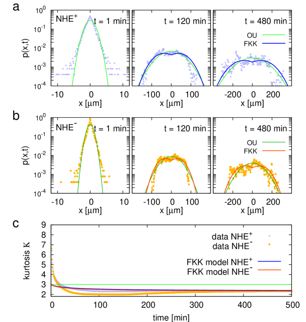
Figure 9: Spatio-temporal probability distributions $P(x,t)$. (a),(b): Experimental data for both cell types at different times in semilogarithmic representation. The dark lines, labeled FKK, show the solutions of our model Eq. (24) with the same parameter set used for the msd fit. The light lines, labeled OU, depict fits by Gaussian distributions representing the theory of Brownian motion. For $t=1$min both $P(x,t)$ show a peaked structure clearly deviating from a Gaussian form. (c) The kurtosis $\kappa(t)$ of $P(x,t)$, plotted as a function of time, saturates at a value different from the one of Brownian motion (line at $\kappa=3$). The other two lines represent $\kappa(t)$ obtained from our model Eq. (24) [Die08].

We next show the probability that the cells reach a given position $x$ at time $t$, which corresponds to the temporal development of the spatial probability distribution function $P(x,t)$. Fig. 9 (a), (b) reveals the existence of non-Gaussian distributions at different times. The transition from a peaked distribution at short times to rather broad distributions at long times suggests again the existence of distinct dynamical processes acting on different time scales. The shape of these distributions can be quantified by calculating the kurtosis

$$\kappa(t):=\frac{<x^{4}(t)>}{<x^{2}(t)>^{2}}\quad,$$ (23)

which is displayed as a function of time in Fig. 9 (c). For both cell types $\kappa(t)$ rapidly decays to a constant clearly below three in the long time limit. A value of three would be the result for the spreading Gaussian distributions of the drunken sailor. These findings are another strong manifestation of the anomalous nature of cell migration.

3 Theoretical modeling

We conclude this section with a short discussion of the stochastic model that we have used to fit the experimental data, as was shown in the previous two figures. The model is defined by the fractional Klein-Kramers equation [Bar00]

$$\frac{\partial P}{\partial t}=-\frac{\partial}{\partial x}\left[vP\right]+\frac{\partial^{1-\alpha}}{\partial t^{1-\alpha}}\gamma\left[\frac{\partial}{\partial v}v+v_{th}^{2}\frac{\partial^{2}}{\partial v^{2}}\right]P\quad.$$ (24)

Here $P=P(x,v,t)$ is the probability distribution depending on time $t$, position $x$ and velocity $v$ in one dimension, $\gamma$ is a damping term and $v_{th}=k_{B}T/M$ stands for the thermal velocity of a particle of mass $M$ at temperature $T$, where $k_{B}$ is Boltzmann’s constant. The last term in this equation models diffusion in velocity space, that is, in contrast to the drunken sailors problem here the velocity is not constant but also randomly distributed according to a probability density, which is determined by this equation. Additionally, and again in difference to the simple diffusion equation that we have encountered in Section 1, this equation features two flux terms both in velocity and in position space, see the second and the first term in this equation, respectively. What distinguishes this equation from an ordinary Klein-Kramers equation, which actually is the most general model of Brownian motion in position and velocity space [Ris96], is the presence of a Riemann-Liouville fractional derivative of order $(1-\alpha)$ in front of the last two terms defined by

$$\frac{\partial^{\delta}P}{\partial t^{\delta}}:=\begin{cases}\frac{\partial^{m}P}{\partial t^{m}}&,\quad\delta=m\\ \frac{\partial^{m}}{\partial t^{m}}\left[\frac{1}{\Gamma(m-\delta)}\;\int_{0}^{t}dt^{\prime}\frac{P(t^{\prime})}{(t-t^{\prime})^{\delta+1-m}}\right]&,\quad m-1<\delta<m\end{cases}$$ (25)

with $m\in\mathbb{N}$. Note that for $\alpha=1$ the ordinary Klein-Kramers equation is recovered. The analytical solution of this equation for the msd has been calculated in Ref. [Bar00] to

$$msd(t)=2v_{th}^{2}t^{2}E_{\alpha,3}(-\kappa t^{\alpha})\quad\to\quad 2\frac{D_{\alpha}t^{2-\alpha}}{\Gamma(3-\alpha)}\quad(t\to\infty)$$ (26)

with $D_{\alpha}=v_{th}^{2}/\gamma$ and the generalized Mittag-Leffler function

$$E_{\alpha,\beta}(z)=\sum_{k=0}^{\infty}\frac{z^{k}}{\Gamma(\alpha k+\beta)}\>,\>\alpha\>,\>\beta>0\>,\>z\in\mathbb{C}\quad.$$ (27)

Note that $E_{1,1}(z)=\exp(z)$, hence $E_{\alpha,\beta}(z)$ is a generalized exponential function. We see that for long times Eq. (26) yields a power law, which reduces to the Brownian motion result in case of $\alpha=1$. The analytical solution of Eq. (24) for $P(x,v,t)$ is not known, however, for large friction $\gamma$ this equation boils down to a fractional diffusion equation for which $P(x,t)$ can be calculated in terms of a Fox function [Sch89a]. This solution is what we have used to fit the data. Our modeling is completed by adding what may be called “biological noise” to Eq. (26),

$$msd_{noise}(t):=msd(t)+2\eta^{2}\quad.$$ (28)

This uncorrelated white noise of variance $\eta^{2}$ mimicks both measurement errors and fluctuations of the cell cytoskeleton. The strength of this noise as extracted from the experimental data is larger than the measurement error and determines the dynamics at small time scales, therefore here we see microscopic fluctuations of the cell body in the experiment. The experimental data in Figs. 8, 9 was then consistently fitted by using the four fit parameters $v_{th},\alpha,\gamma$ and $\eta^{2}$ in Bayesian data analysis [Die08].

We consider this model as an interesting illustration of the usefulness of stochastic fractional equations in order to understand real experimental data displaying anomalous dynamics. However, the reader may still wonder about the physical and biological interpretation of the above equation for cell migration. First of all, it can be argued that the fractional Klein-Kramers equation is approximately related to the generalized Langevin equation [Lut01]

$$\dot{v}=-\int_{0}^{t}dt^{\prime}\>\gamma(t-t^{\prime})v(t^{\prime})+\sqrt{\zeta}\>\xi(t)\quad.$$ (29)

This equation can be understood as a stochastic version of Newton’s law: The left hand side holds for the acceleration of a particle, whereas the total force acting onto it is decomposed into a friction term and a random force. The latter is modeled by Gaussian white noise $\xi(t)$ of strength $\sqrt{\zeta}$, and the friction coefficient is time-dependent obeying a power law, $\gamma(t)\sim t^{-\alpha}$. The friction term could thus be written again in form of a fractional derivative. Note that for $\gamma=const.$ the ordinary Langevin equation is recovered, which is a standard model of Brownian motion [Rei65, Ris96]. This relation suggests that physically the anomalous cell migration could have its origin, at least partially, in the existence of a memory-dependent friction coefficient. The latter, in turn, might be explained by anomalous rheological properties of the cell cytoskeleton, which consists of a complex biopolymer gel [Sem07].

Secondly, what could be the possible biological significance of the observed anomalous cell migration? Both the experimental data and the theoretical modeling suggest that there exists a slow diffusion on small time scales, whereas the long-time motion is much faster. In other words, the dynamics displays intermittency qualitatively similar to the one outlined in Section 1. Interestingly, there is an ongoing discussion about optimal search strategies of foraging animals such as albatrosses, marine predators and fruit flies, see, e.g., Ref. [Edw07] and related literature. Here it has been argued that Lévy flights, which define a fundamental class of anomalous dynamics [Kla08], are typically superior to Brownian motion for animals in order to find food sources. However, more recently it was shown that under certain circumstances intermittent dynamics is even more efficient than pure Lévy motion [Bén06]. The results on anomalous cell migration presented above might thus be biologically interpreted within this context.

Chapter 4 Summary

This review has covered a rather wide range of topics and methods: Chapter 1 has introduced to the concept of deterministic chaos by defining and calculating fundamental quantities characterizing chaos such as Ljapunov exponents and dynamical entropies. These quantities were shown to be intimately related to each other as well as to properties of fractal sets. Chapter 2 started by reminding of simple random walks on the line, their characterization in terms of diffusive properties, and the relation to elementary concepts of Brownian motion. These basic ideas were then discussed in a chaotic setting in form of deterministic diffusion. A formula was derived exactly expressing diffusion in terms of the chaos quantities introduced in the previous chapter. Chapter 3 generalized the concept of normal diffusion leading to anomalous diffusion. A simple deterministic model generating this type of diffusion was introduced and analyzed both numerially and by means of stochastic theory. For the latter purpose, continuous time random walk theory was explained and applied leading to a generalized, fractional diffusion equation. As an example of experimental applications of these concepts, anomalous biological cell migration was discussed. Experimental results for the mean square displacement and for the probability distribution in position space matched nicely to the predictions of a stochastic model in form of a fractional diffusion equation, defined both in position and velocity space. The scope of this review thus spans from very simple, abstract models to experiments and from basic dynamical systems theory to advanced methods of stochastic analysis.

Of course, this work poses a wealth of open questions. Here we restrict ourselves to only one of them which we consider to be of particular importance: We could understand the origin of normal diffusion in terms of microscopic deterministic chaos by applying a combination of methods from statistical physics and dynamical systems theory; but what’s about anomalous diffusion? To our knowledge, yet there is no analogous theory available, like the escape rate formalism for normal diffusion, which explains the origin of anomalous diffusion in terms of weak chaos. This is the reason why here we restricted ourselves to applying numerical and stochastic methods to an anomalous deterministic model. We believe that constructing such a microscopic dynamical systems theory of anomalous deterministic transport poses a big challenge for future work in this field.

Acknowledgements:
The author gratefully acknowledges the long-term collaboration with J.R.Dorfman leading to the material presented in Chapter 2. He also wishes to thank his former Ph.D. student N.Korabel for help with some of the figures and for joint work on Section 1, which formed part of his Ph.D. thesis. A.V.Chechkin significantly contributed to the same section but in particular introduced the author to the stochastic theory of anomalous diffusion, for which he is extremely grateful. P.Dieterich was the main driving force behind the project reviewed in Section 2, and the author thanks him for highly interesting joint work on crawling cells. Finally, he thanks his former postdoc P.Howard for help with some figures and particularly for recent first steps towards solving the question posed above.

References

- [All97] K.T. Alligood, T.S. Sauer and J.A. Yorke, Chaos - An introduction to dynamical systems. (Springer, New York, 1997).
- [Arn68] V.I. Arnold and A. Avez, Ergodic problems of classical mechanics. (W.A. Benjamin, New York, 1968).
- [Bad97] R. Badii and A. Politi, Complexity: hierarchical structures and scaling physics. (Cambridge University Press, Cambridge, 1997).
- [Bar00] E. Barkai and R. Silbey, Fractional Kramers Equation. J. Phys. Chem. B 104, 3866––3874 (2000).
- [Bec93] C. Beck and F. Schlögl, Thermodynamics of Chaotic Systems, volume 4 of Cambridge nonlinear science series. (Cambridge University Press, Cambridge, 1993).
- [Bén06] O. Bénichou, M. Coppey, M. Moreau and R. Voituriez, Revisiting Lévy flight search patterns of wandering albatrosses, bumblebees and deer. Europhys. Lett. 75, 349––354 (2006).
- [Bou90] J.-P. Bouchaud and A. Georges, Anomalous diffusion in disordered media: Statistical mechanisms, models and physical applications. Phys. Rep. 195, 127–293 (1990).
- [Bun08] L. Bunimovich and A. Yurchenko, Where to place a hole to achieve a maximal escape rate. preprint arXiv.org:0811.4438, 2008.
- [Dev89] R.L. Devaney, An introduction to chaotic dynamical systems. (Addison-Wesley, Reading, second edition, 1989).
- [Die08] P. Dieterich, R. Klages, R. Preuss and A. Schwab, Anomalous dynamics of cell migration. PNAS 105, 459–463 (2008).
- [Dor99] J.R. Dorfman, An introduction to chaos in nonequilibrium statistical mechanics. (Cambridge University Press, Cambridge, 1999).
- [Dun87] G.A. Dunn and A.F. Brown, A unified approach to analysing cell motility. J. Cell Sci. Suppl. 8, 81–102 (1987).
- [Ebe05] W. Ebeling and I.M. Sokolov, Statistical thermodynamics and stochastic theory of nonequilibrium systems. (World Scientific, Singapore, 2005).
- [Eck85] J.-P. Eckmann and D. Ruelle, Ergodic theory of chaos and strange attractors. Rev. Mod. Phys. 57, 617–656 (1985).
- [Edw07] A. Edwards et al., Revisiting Lévy flight search patterns of wandering albatrosses, bumblebees and deer. Nature 449, 1044–1048 (2007).
- [Ein05] A. Einstein, Über die von der molekularkinetischen Theorie der Wärme geforderten Bewegung von in ruhenden Flüssigkeiten suspendierten Teilchen. Annalen der Physik 17, 549–560 (1905).
- [Fal90] K. Falconer, Fractal geometry. (Wiley, New York, 1990).
- [Fal05] M. Falcioni, L. Palatella and A. Vulpiani, Production rate of the coarse-grained Gibbs entropy and the Kolmogorov-Sinai entropy: A real connection? Phys. Rev. E 71, 016118/1–8 (2005).
- [Gas90] P. Gaspard and G. Nicolis, Transport properties, Lyapunov exponents, and entropy per unit time. Phys. Rev. Lett. 65, 1693–1696 (1990).
- [Gas98] P. Gaspard, Chaos, scattering, and statistical mechanics. (Cambridge University Press, Cambridge, 1998).
- [Gei84] T. Geisel and S. Thomae, Anomalous diffusion in intermittent chaotic systems. Phys. Rev. Lett. 52, 1936–1939 (1984).
- [Gei85] T. Geisel, J. Nierwetberg and A. Zacherl, Accelerated diffusion in Josephson junctions and related chaotic systems. Phys. Rev. Lett. 54, 616–619 (1985).
- [Har94] R.S. Hartmann, K. Lau, W. Chou and T.D. Coates, The fundamental motor of the human neutrophil is not random: Evidence for local non-Markov movement in neutrophils. Biophys. J. 67, 2535–2545 (1994).
- [Jen04] O. Jenkinson and M. Pollicott, Entropy, exponents and invariant densities for hyperbolic systems: dependence and computation. in: Y. Pesin M. Brin, B. Hasselblatt, Eds., Modern Dynamical Systems and Applications, pages 365–384, Cambridge University Press, Cambridge, 2004.
- [Kan85] H. Kantz and P. Grassberger, Repellers, semi-attractors, and long-lived chaotic transients. Physica D 17, 75–86 (1985).
- [Kat95] A. Katok and B. Hasselblatt, Introduction to the modern theory of dynamical systems, volume 54 of Encyclopedia of Mathematics and its Applications. (Cambridge University Press, Cambridge, 1995).
- [Kla95] R. Klages and J.R. Dorfman, Simple maps with fractal diffusion coefficients. Phys. Rev. Lett. 74, 387–390 (1995).
- [Kla96a] J. Klafter, M. F. Shlesinger and G. Zumofen, Beyond Brownian motion. Phys. Today 49, 33–39 (1996).
- [Kla96b] R. Klages, Deterministic diffusion in one-dimensional chaotic dynamical systems. (Wissenschaft & Technik-Verlag, Berlin, 1996).
- [Kla97] R. Klages and J.R. Dorfman, Dynamical crossover in deterministic diffusion. Phys. Rev. E 55, R1247–R1250 (1997).
- [Kla99] R. Klages and J.R. Dorfman, Simple deterministic dynamical systems with fractal diffusion coefficients. Phys. Rev. E 59, 5361–5383 (1999).
- [Kla07a] R. Klages, Introduction to dynamical systems. Lecture notes, see http://www.maths.qmul.ac.uk/klages/teaching/mas424, 2007.
- [Kla07b] R. Klages, Microscopic chaos, fractals and transport in nonequilibrium statistical mechanics, volume 24 of Advanced Series in Nonlinear Dynamics. (World Scientific, Singapore, 2007).
- [Kla08] R. Klages, G. Radons and I.M. Sokolov, Eds., Anomalous transport. (Wiley-VCH, Berlin, 2008).
- [Kor05] N. Korabel, A.V. Chechkin, R. Klages, I.M. Sokolov and V.Yu. Gonchar, Understanding anomalous transport in intermittent maps: From continuous time random walks to fractals. Europhys. Lett. 70, 63–69 (2005).
- [Kor07] N. Korabel, R. Klages, A.V. Chechkin, I.M. Sokolov and V.Yu. Gonchar, Fractal properties of anomalous diffusion in intermittent maps. Phys. Rev. E 75, 036213/1–14 (2007).
- [Las94] A. Lasota and M.C. Mackay, Chaos, Fractals, and Noise. (Springer-Verlag, 1994).
- [Lut01] E. Lutz, Fractional Langevin equation. Phys. Rev. E 64, 051106/1–4 (2001).
- [Mai97] F. Mainardi, Fractional Calculus: some Basic Problems in Continuum and Statistical Mechanics. in: A. Carpinteri and F. Mainardi, Eds., Fractals and Fractional Calculus in Continuum Mechanics, Springer, New York, 1997.
- [Man82] B.B. Mandelbrot, The fractal geometry of nature. (W.H. Freeman and Company, San Francisco, 1982).
- [Met00] R. Metzler and J. Klafter, The random walk’s guide to anomalous diffusion: A fractional dynamics approach. Phys. Rep. 339, 1–77 (2000).
- [Mon65] E.W. Montroll and G.H. Weiss, Random walks on lattices II. J. Math. Phys. 6, 167–179 (1965).
- [Mon73] E.W. Montroll and H. Scher, Random walks on lattices IV: Continuous-time walks and influence of absorbing boundaries. J. Stat. Phys. 9, 101–133 (1973).
- [Ott93] E. Ott, Chaos in Dynamical Systems. (Cambridge University Press, Cambridge, 1993).
- [Pea05] K. Pearson, The problem of the random walk. Nature 72, 294, 342 (1905).
- [Per09] J.-B. Perrin, Mouvement brownien et réalité moléculaire. Ann. Chim. Phys. 19, 5–104 (1909).
- [Pod99] I. Podlubny, Fractional differential equations. (Academic Press, New York, 1999).
- [Pom80] Y. Pomeau and P. Manneville, Intermittent transition to turbulence in dissipative dynamical systems. Commun. Math. Phys. 74, 189–197 (1980).
- [Ray05] J.W. Strutt (Lord Rayleigh), The problem of the random walk. Nature 72, 318 (1905).
- [Rei65] F. Reif, Fundamentals of statistical and thermal physics. (McGraw-Hill, Auckland, 1965).
- [Ris96] H. Risken, The Fokker-Planck Equation. (Springer, Berlin, 2nd edition, 1996).
- [Rob95] C. Robinson, Dynamical Systems. (CRC Press, London, 1995).
- [Sch75] H. Scher and E.W. Montroll, Anomalous transit-time dispersion in amorphous solids. Phys. Rev. B 12, 2455–2477 (1975).
- [Sch89a] W.R. Schneider and W.Wyss, Fractional diffusion and wave equations. J. Math. Phys 30, 134––144 (1989).
- [Sch89b] H.G. Schuster, Deterministic chaos. (VCH Verlagsgesellschaft mbH, Weinheim, 2nd edition, 1989).
- [Sem07] C. Semmrich, T. Storz, J. Glaser, R. Merkel, A.R. Bausch and K. Kroy, Glass transition and rheological redundancy in F-actin solutions. PNAS 104, 20199–20203 (2007).
- [Shl85] M.F. Shlesinger and J. Klafter, Accelerated diffusion in Josephson-junctions and related chaotic systems - comment. Phys. Rev. Lett. 54, 2551 (1985).
- [Shl93] M.F. Shlesinger, G.M. Zaslavsky and J. Klafter, Strange kinetics. Nature 363, 31–37 (1993).
- [Sok02] I.M. Sokolov, J. Klafter and A. Blumen, Fractional kinetics. Phys. Today 55, 48–54 (2002).
- [Sto91] C.L. Stokes and S.K. Williams D.A. Lauffenburger, Migration of individual microvessel endothelial cells: Stochastic model and parameter measurement. J. Cell Science 99, 419–430 (1991).
- [Tél90] T. Tél, Transient Chaos. in: B.-L. Hao, Eds., Experimental Study and Characterization of Chaos, volume 3 of Directions in chaos, pages 149–211. (World Scientific, Singapore, 1990).
- [Tod92] M. Toda, R. Kubo and N. Saitô, Statistical Physics, volume 1 of Solid State Sciences. (Springer, Berlin, 2nd edition, 1992).
- [Tri95] C. Tricot, Curves and fractal dimension. (Springer, Berlin, 1995).
- [Upa01] A. Upadhyaya, J.P. Rieu, J.A. Glazier and Y. Sawada, Anomalous diffusion and non-Gaussian velocity distributions of Hydra cells in cellular aggregates. Physica A 293, 549–558 (2001).
- [Wei94] G.H. Weiss, Aspects and applications of the random walk. (North-Holland, Amsterdam, 1994).
- [You02] L.-S. Young, What are SRB measures, and which dynamical systems have them? J. Stat. Phys. 108, 733–754 (2002).
- [Zum93] G. Zumofen and J. Klafter, Scale-invariant motion in intermittent chaotic systems. Phys. Rev. E 47, 851–863 (1993).