Double Exchange Model at Low Densities: Magnetic Polarons and Coulomb Suppressed Phase Separation

Abstract

We consider the double exchange model at very low densities. The conditions for the formation of self-trapped magnetic polarons are analyzed using an independent polaron model. The issue of phase separation in the low density region of the temperature-density phase diagram is discussed. We show how electrostatic and localization effects can lead to the substantial suppression of the phase separated regime. By examining connections between the resulting phase and the polaronic phase, we conclude that they reflect essentially the same physical situation of a ferromagnetic droplet containing one single electron. In the ultra diluted regime, we explore the possible stabilization of a Wigner crystal of magnetic polarons. Our results are compared with the experimental evidence for a polaronic phase in europium hexaboride ($\mathrm{EuB_{6}}$), and we are able to reproduce the experimental region of stability of the polaronic phase. We further demonstrate that phase-separation is a general feature expected in metallic ferromagnets whose bandwidth depends on the magnetization.

I Introduction

The earliest descriptions of the concept of magnetic polaron appear with the considerations by de Gennes on the relevance of the double exchange (DE) mechanism to the mixed valent manganites de Gennes (1960), and then with Nagaev’s studies of antiferromagnetic semiconductors, who coined the term ferron also often used in the context Nagaev (2001, 2002). Some of the first theories based upon the presence of magnetic polarons were developed later in the context of the ferromagnetic semiconductor EuO, to explain the spectacular metal-insulator transition found at the onset of ferromagnetism for the Eu-rich samples of this compound Oliver et al. (1972); Torrance et al. (1972). Further developments on this concept permitted the explanation of the spin-flip Raman scattering characteristic of certain diluted magnetic semiconductors (DMS) Dietl and Spalek (1982, 1983); Heiman et al. (1983); Torrance et al. (1972) and, more recently, their presence was also claimed to be present in the $\mathrm{EuB_{6}}$ hexaborides Snow et al. (2001); Nyhus et al. (1997).

Just as in the analogous case of the electrostatic polaron, one can devise a pictorial description of a magnetic polaron in real space, consisting of a charge carrier surrounded by a cloud of polarized local spins in an unpolarized magnetic background — a state that arises from the exchange interaction between the carrier spin and the lattice spins. A distinction is usually made between the so-called bound magnetic polaron (BMP) and the free magnetic polaron (FMP). The BMP is invoked when the charge carrier is bound via Coulomb interaction to an impurity center, and is typical in the magnetic semiconductors. In this case the trapped carrier polarizes the lattice spins within its effective Bohr radius as a consequence of the s–d-like interaction between electron and lattice spins. The FMP, by contrast, results from the fact that a free carrier interacting with lattice spins via an s–d coupling, can minimize its kinetic energy by polarizing its vicinity. Under certain conditions this carrier can then become self-trapped in the resulting potential well created by the effect of the local ferromagnetism.

The presence of such type of entities is believed to play an important role in the emergence of many interesting properties of several important magnetic materials: many peculiarities of the manganites, such as the colossal magnetoresistance (CMR) effect and other anomalies in its transport and magnetism, have been attributed in part to the development of magnetic polarons near the ferromagnetic transition (although in this case the influence of orbital and lattice degrees of freedom is equally important) Teresa et al. (1997); Amaral et al. (1998); Teresa et al. (2000); an interpretation for the CMR in the Mn pyrochlores was also proposed on the basis of magnetic polarons Majumdar and Littlewood (1998); besides their relevance for the already mentioned Eu-chalcogenides and II-VI semiconductors, in the III-V DMS like Ga_1-xMn_xAs, the ferromagnetic transition can be interpreted within a BMP percolating scenario Kaminski and Sarma (2002); in $\mathrm{EuB_{6}}$, our target magnetic metal exhibiting CMR, their presence in signaled in the optical response Nyhus et al. (1997); Snow et al. (2001), although the theoretical interpretation of these results has been subject to questioning Calderón et al. (2004).

Given that these different classes of magnetic materials have attracted considerable attention in recent years because of their potential for the development of new magnetoelectronic devices, and since magnetic polarons have an apparently ubiquitous presence among them, a number of theoretical approaches to the problem have been developed through the years. In particular, extensive work has been done with emphasis in the physics of magnetic semiconductors Kasuya et al. (1970); Dietl and Spalek (1982); Heiman et al. (1983); Mauger (1983); Nagaev (2002) and CMR manganites Varma (1996); Batista et al. (2000); Garcia et al. (2002); Meskine et al. (2004).

In the ensuing sections we will focus our attention on the stability conditions for the free magnetic polaron in the double exchange model (DEM), with an eye on the experimental evidence for magnetic polarons in $\mathrm{EuB_{6}}$ Nyhus et al. (1997); Snow et al. (2001), and having in mind the description of the magneto-electronic properties of this material in terms of DE V. M. Pereiraet al. (2004). Studies devoted to the polaronic stability in this particular model and its variations have been performed by several authors both analytically and numerically, although under different assumptions Daghofer et al. (2004a, b); Garcia et al. (2002); Koller et al. (2003); Neuber et al. (2004); Pathak and Satpathy (2001); Wang and J.Freeman (1997); Yi et al. (2000). We show that the DE-based interpretation of magnetotransport in $\mathrm{EuB_{6}}$ is consistent with the experimental evidence for a polaronic phase mediating the PM-FM transition. In particular, within an independent polaron model (IPM) we reproduce the experimental temperature and density range of the polaronic phases, without adjusting parameters.

Given that we are focusing on the low density regime of the DEM, another issue becomes pressing: the known tendency for this model to exhibit a phase separation instability at reduced densities Nagaev (1998); Yunoki et al. (1998); Arovas et al. (1999); Kagan et al. (1999); Alonso et al. (2001a, b). We characterize the phase-separated regime and study how the introduction of electrostatic corrections leads to considerable shrinking of the phase separation region in the phase diagram. We discuss how the phase-separated regime is connected and compatible with the polaronic phase.

This paper is organized in the following manner. In Sec. II we briefly introduce some experimental details regarding electronic transport and magnetism in $\mathrm{EuB_{6}}$, only to the extent of motivating our studies. In Sec. IV we introduce and discuss an IPM for the DEM at very low densities, whose results are then confronted in Sec. IV with the experimental evidence for magnetic polarons in $\mathrm{EuB_{6}}$. We then address the problem of phase separation in the low-density DEM in Sec. V: we discuss the emergence of phase separation at low densities, study its suppression when electrostatic corrections are taken into consideration and explore the connections of the resulting phase with the polaronic phase. We consider the ultra diluted regime in Sec. VI, and provide estimates for the stability of a Wigner crystal of magnetic polarons. In Sec. VII we close this paper with our conclusions.

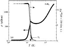
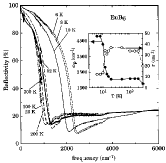
Figure 1: Some experimental signatures of $\mathrm{EuB_{6}}$. Panel 1 shows the behavior of the DC resistivity and magnetic susceptibility as a function of temperature, as reproduced in LABEL:~Paschen et al., 2000. Notice the upturn followed by a massive drop in $\rho(T)$ at $T_{\text{C}}$, which correlates with the onset of magnetic order. In 1 we reproduce the results from LABEL:~Degiorgi et al., 1997 for the optical reflectivity at different temperatures. The enhancement of $\omega_{\text{p}}$ as the system becomes magnetic is clear.

II Overview of EuB${}_{\text{6}}$ Properties

We briefly review the physics of $\mathrm{EuB_{6}}$ that motivates our choice of microscopic model. An extensive review of the phenomenology of this material was given in LABEL:~Pereira, 2006, and here we limit ourselves to the essential aspects relevant in the context of this paper. $\mathrm{EuB_{6}}$ is a magnetic metalFisk et al. (1979); Guy et al. (1980), with residual resistivities at $T\to 0$ of the order of $\sim 10\mu\Omega.\text{cm}$, or less, and exibiths a clear CMR signal close to $T_{\text{C}}$Süllow et al. (1998); Aronson et al. (1999) [Fig. 1]. Notwithstanding, $\mathrm{EuB_{6}}$ has a very small carrier density. More precisely, carrier densities estimated from Hall effect measurements amount to as little as $\sim 10^{19}\text{cm}^{-3}$, or $\sim 0.001$ carriers per unit cell Fisk et al. (1979); Paschen et al. (2000); Rhyee et al. (2003a). These conduction electrons are believed to arise from the presence of defects in the structural arrangement of the boron framework Blomberg et al. (1995); Monnier and Delley (2001). Such defects generate a surplus of electrons that occupy states in the conduction band.

One of the most intriguing and peculiar features of $\mathrm{EuB_{6}}$ is arguably the giant and rather unusual blue-shift of the unscreened plasma edge, $\omega_{\text{p}}$, induced simply by a temperature variation (Broderick et al., 2003; Degiorgi et al., 1997) [Fig. 1]. At $T>T_{\text{C}}$, the reflectivity spectrum displays a typical metallic behavior, with a very well defined plasma threshold. With the establishment of the long-range magnetic order, the plasma edge increases markedly in such a way that $\omega_{\text{p}}$varies by a factor of almost 3 between $T_{\text{C}}$ and $T\ll T_{\text{C}}$ (Broderick et al., 2002; Degiorgi et al., 1997). This variation of $\omega_{\text{p}}$ is consistent with the remarkable enhancement in the carrier densities as the temperature is lowered past $T_{\text{C}}$Paschen et al. (2000).

The conduction and valence bands of $\mathrm{EuB_{6}}$ are separated by a gap of the order of 1 eV Denlinger et al. (2002); Giannò et al. (2002); Souma et al. (2003); Rhyee et al. (2003b). This fundamental gap lies at the $X$ point in the cubic Brillouin zone (BZ), and the close proximity of $E_{\text{F}}\,$to the bottom of the conduction band dictates a pocket-like structure for the Fermi surface. Given that the interest will be almost completely in a temperature range $T\lesssim T_{\text{C}}$, the electronic states in the valence band are disregarded in the following.

The magnetism of $\mathrm{EuB_{6}}$ arises entirely from the half-filled $4f$ shell of Eu²⁺ in the state ${}^{8}S_{7/2}$. This implies localized magnetism stemming from magnetic moments of magnitude $S=7/2$. Within this formulation these electrons do not itinerate at all. We designate the resulting magnetic moment by local spin, and use the term magnetization of the system when alluding to long range ordered phases of these spins. In addition, for our purposes the conduction band electrons interact with the local spins only through the Hund’s coupling between the electron’s spin and the local moments’.

III The Independent Polaron Model

The Hamiltonian describing conduction electrons hopping in a tridimensional cubic lattice, and coupled to local spins at each lattice site is

$$\mathcal{H}_{\,{}_{KLM}} =\sum_{\left<i,j\right>,\sigma}t_{i,j}\;c^{\dagger}_{i,\sigma}c_{j,\sigma}+\text{h.c.}$$

$$+J_{H}\sum_{i,\alpha,\beta}\vec{S}_{i}\,\cdot\vec{\tau}_{\alpha,\beta}\;c^{\dagger}_{i,\alpha}c_{i,\beta}\,,$$ (1)

usually known as $s-f$ or Kondo lattice model (KLM) Hamiltonian (Doniach, 1977), and is one of the canonical models in correlated electronic systems. In this expression, $t_{i,j}\equiv t$ is the hopping integral between neighboring lattice sites, $c^{\dagger}_{i,\sigma}(c_{i,\sigma})$ are the second-quantized fermionic creation (annihilation) operators at latice site $i$, $\vec{S}_{i}\,$represents the local magnetic moment of magnitude $S=7/2$, $J_{H}$ the exchange coupling of the latter to the itinerating electrons, and $\vec{\tau}=(\tau_{1},\tau_{2},\tau_{3})$ is the vector of Pauli matrices. The sum in the first term is over all pairs of nearest neighboring sites $\left<i,j\right>$.

Since $S=7/2$ is a rather high spin, the local spin operator is replaced by the classical vector $\vec{S}_{i}\,$, parametrized with spherical angles as $\vec{S}_{i}\,=S\bigl{(}\sin(\theta_{i})\cos(\varphi_{i}),\sin(\theta_{i})\sin(\varphi_{i}),\cos(\theta_{i})\bigr{)}$. This transforms the second term in (1) into a generalized potential term for the electrons, which will be a disordered potential above $T_{\text{C}}$, where all $\vec{S}_{i}\,$are uncorrelated. Furthermore, the magnetic and electronic time scales are well apart in such a way that the magnetic background provided by the $\vec{S}_{i}\,$is essentially quenched. This means that the typical time between spin fluctuations is much longer than the time for the electronic subsystem to reach its ground state

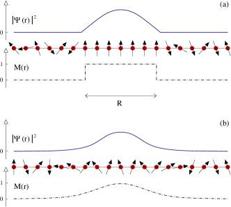
Figure 2: Contrasting the variational approach considered in eq. (6) (a) to the more realistic, self-consistent, situation (b). Represented are the wave function of the self-localized electron, a possible spin configuration and the magnetization profile.

Under these circumstances, we consider the effective DE Hamiltonian de Gennes (1960); Hasegawa and Yanase (1979) that obtains in the limit $J_{H}\to\infty$. This is accomplished through a local rotation of the quantization axis so that it coincides with the direction of $\vec{S}_{i}\,$at each site, and projecting out the anti-parallel electron states Dagotto (2003). Such anti-parallel states lie higher in energy (by $\approx J_{H}$) and hence are suppressed in the effective Hilbert space. The result is

$$\mathcal{H}_{DE}=t\sum_{\langle ij\rangle}a_{ij}d^{\dagger}_{i}d_{j}+\text{H. c.}\,,$$ (2)

where the new operators $d_{i}$ correspond to an effective spinless electron that maintains its spin aligned with each local moment, and all information about the magnetic background is condensed in the effective hopping amplitude $a_{ij}$:

$$a_{ij}=\cos\left(\frac{\theta_{i}}{2}\right)\cos\left(\frac{\theta_{j}}{2}\right)+\sin\left(\frac{\theta_{i}}{2}\right)\sin\left(\frac{\theta_{j}}{2}\right)e^{-i(\phi_{i}-\phi_{j})}\,.$$ (3)

Within the simple DEM, where no other polaron-favoring interactions are included (e.g. not including antiferromagnetic (AFM) exchange terms between the local moments.), the only possibility for the stabilization of magnetic polarons is at low electronic densities. This happens because the local spins of several neighboring unit cells are expected to participate in the magnetization cloud of each electron. Were it otherwise (i.e. at high electronic densities), the electronic wave functions would overlap considerably destroying this polaron picture.

In order to investigate this problem we will first discuss the thermodynamic stability of magnetic polarons within the DEM. We can write a free energy for the system including an electronic contribution consisting of the ground state energy for the electrons in a given magnetic configuration, the local spins contributing only with an entropic term. To tackle the first part, we calculate numerically the exact electronic density of states (DOS) for a given spin configuration Pereira (2006), which we designate by $\rho\bigl{(}E,\{\vec{S}_{i}\,\}\bigr{)}$, and extract the disorder-averaged DOS at constant magnetization: $\rho\bigl{(}E,M)$ ($M$ being the normalized local magnetization) (details about this numerical calculation will be given below in Sec. V.1).

With this averaging over disorder, we can write the electronic contribution to the free energy as

$$E_{el}(M,n_{e})=\int\Theta\Bigl{(}E_{F}(M,n_{e})-\epsilon\Bigr{)}E\rho(E,M)dE\,,$$ (4)

where the dependence of the Fermi energy on both magnetization and electron density was made explicit. When $n_{e}\ll 1$, and for the purposes of the current calculation, Eq. (4) can be approximated simply by

$$E_{el}(M,n_{e})\approx E_{b}(M)n_{e}\,,$$ (5)

with $E_{b}$ representing the bottom of the band – it becomes just a single electron problem. Indeed, given the nature of the calculation and approximations involved here, the consideration of the finite band filling introduces only minor corrections and thus we proceed with the above approximation to the electronic energy (Appendix A). Now, for a disordered system, the concept of “bottom of the band” has to be taken carefully as the DOS will always exhibit Lifshitz exponential tails. In this case, from the calculations of the averaged DOS, the bottom of the band is found to lie at $-4t$ for the paramagnetic (PM) ($M=0$) case End (a) (cfr. Fig. 5). We intend to construct the polaronic phase having the paramagnetic, uniform, phase as reference. Within a virtual-crystal approximation, the electron at the bottom of the band has an energy of $-4t$, and will be extended throughout the system. If a region of ferromagnetism develops locally, its reference energy in this region will be lowered to $-6t$, but there is an extra energy that has to be paid if the electron is to become confined to this region. For simplicity let us assume that the polaron so formed consists of a region inside a cube of side $R$ (in units of the lattice parameter, $a$), inside which $M=1$. Obviously, given that in the DEM the magnetic interaction is mediated by electron itinerancy, one expects that, once the electron localizes inside this cube, there will be no magnetism outside, at any temperature. The variation of free energy per lattice site when going from the PM homogeneous phase to this polaronic one will be written as

$$\Delta\mathcal{F}_{\textrm{Pol}}(R,T)=4tn_{e}-6tn_{e}\cos\left(\frac{\pi}{R+1}\right)+Tn_{e}R^{3}\log(2S+1)-T\mathcal{S}_{\textrm{Cfg}}(n_{e},R)\,,$$ (6)

and reflects the two competing effects at play: the first is the electron’s preference for a ferromagnetic background accompanied by an energy cost for the localization; the second is the reduction of entropy caused by the appearance of the (fully polarized) magnetic polarons. The last contribution, $\mathcal{S}_{\textrm{Cfg}}$, expresses a configurational entropy, related to the spacial distribution of the polarons inside the system. It is a combinatorial term that can be approximated by

$$\mathcal{S}_{\textrm{Cfg}}\simeq\frac{1}{R^{3}}\log\left(\frac{1}{1-n_{e}R^{3}}\right)-n_{e}\log\left(\frac{n_{e}R^{3}}{1-n_{e}R^{3}}\right)\,,$$ (7)

but, since we are working with $n_{e}\ll 1$ and the polaronic system is below the percolation threshold, it happens to be the smallest contribution to $\Delta\mathcal{S}$, allowing us to neglect it without important quantitative consequences.

In writing eq. (6) some important assumptions were made regarding the wave function of the electron. Reasoning in terms of the original band state of the electron, it is clear that when the magnetic background polarizes, the electron energy is lowered by $2t$. Thus, the potential well is, at most, $2t$ deep and any bound state will always exhibit exponential leaking of the wave function to the outside, whereas the energy of the bound state in (6) was chosen as the energy of an electron inside an infinite potential well. On the other hand, since one can think of an effective magnetic coupling as proportional to $\left|\psi_{e}(\vec{r})\right|^{2}$, the magnetization profile of the polaron should also display a smooth variation, whereas in eq. (6) $M=0$ outside and $M=1$ inside the polaron (cfr. Fig. 2). These statements amount to say that the exact treatment of the problem requires a self-consistent calculation of the bound state starting from the DEM or perhaps from the full Hamiltonian Kasuya et al. (1970); Pathak and Satpathy (2001). In this sense, eq. (6) is to be understood in the spirit of a variational approach, $R$ being the variational parameter.

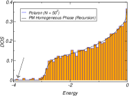
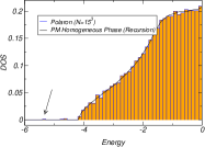
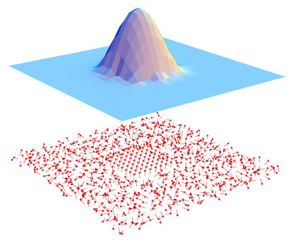
Figure 3: Comparison of the disorder-averaged electronic DOS for the homogeneous PM phase (line) with the exact spectrum obtained for the same configuration with a polaronic region or size $R$ (histogram). Arrows highlight the lowest bound state. The results in 3 are for 2D and $R=9$, and in 3 for 3D, $R=5$. The histogram was obtained from the full numerical diagonalization of the polaronic configuration. The continuous line represents the bulk DOS obtained with the recursion method. For this comparison we neglected the Berry phase in the hopping (i.e. we used $a_{ij}\rightarrow\left|a_{ij}\right|$). Panel 3 shows one of those 2D spin configurations in the polaronic phase (bottom) together with the corresponding exact wavefunction of the lowest bound state (top).

There are several reasons to expect it to be a good approximation: (i) the electron density is very small, meaning that the overlap of the wave functions of self-trapped electrons (and thus the polarons) should be negligible; (ii) even if one could devise a full, self-consistent, solution to the problem, the exact energy of the bound state is expected to differ from the one used in this approximation only by numerical factors of $\mathcal{O}(1)$. Specific confirmation for this can be found, for instance, in the 1-D calculations of Pathak and Satpathy (2001), who find that the two energies (calculated using the same kind of variational wave function used in the current work and the exact energy obtained numerically) differ by less than 3 % in the limit relevant to our discussion. ; (iii) numerical calculations strongly favor this approach. To dwell a while on this last point, we studied the effect of a region of full polarization embedded in a PM background on the electronic spectrum. Performing exact diagonalizations of the DEM using spin configurations like the one depicted in Figs. 2 and 3, one finds, as a result, the appearance of well defined bound states below the continuum band. This is clearly seen in Figs. 3 and 3, where the bound states appear with energies and degeneracy coinciding with the value expected for a finite box in $d\textrm{-dimensions}$: $-2dt\sum_{\mu=1}^{d}\cos\left(\frac{\pi}{R+1}n_{\mu}\right)$. At the same time, inspecting particular realizations of disorder as the one in Fig. 3, one concludes that the wave function is clearly localized within the polarized region, thus supporting our trial function selection for the evaluation of the electronic energy.

The stability of the magnetic polaron is determined by the condition $\Delta\mathcal{F}\left(R_{\textrm{eq}},T\right)<0$, $R_{\textrm{eq}}$ being the value that minimizes the free energy (6). Important insights can be extracted from the direct analytic results obtainable in its continuum version (i.e. $R\gg 1$). In this case the equilibrium radius is

$$R_{\textrm{eq}}\left(T\right)\simeq\left[\frac{2t\pi^{2}}{T\log\left(2S+1\right)}\right]^{1/5}\,,$$ (8)

increasing at low temperatures as $T^{-1/5}$. This power law behavior of $R_{\text{eq}}$ with temperature is reminiscent of the one found in the context of magnetic semiconductors Kasuya et al. (1970). Using this result in the stability condition, one finds the stability temperature, $T_{m}$, below which the polaronic phase appears:

$$T_{m}=\frac{8}{25\pi^{3}\log\left(2S+1\right)}\sqrt{\frac{2}{5}}t\,.$$ (9)

These two results convey the essential information for the physical situation as one reduces the temperature of our system. The high-temperature phase is characterized by PM order until $T$ decreases below $T_{m}$, at which point, the “entropic pressure” is not enough to counteract the energy gain and the polaronic phase is stabilized. The transition is sharp as a consequence of the one-particle nature of the free energy (6), and the polarons set in with a finite radius $R_{\textrm{eq}}\left(T_{m}\right)$. Continuing the decrease in temperature, the polaron radius increases until the overlapping probability can no longer be ignored, therefrom arising an instability towards an homogeneous ferromagnetic (FM) phase. An estimate of the Curie temperature, $T_{\text{C}}$, can thus be extracted from a percolation criterion

$$n_{e}R_{\textrm{eq}}\left(T_{C}\right)^{3}\simeq p_{c}\,,$$ (10)

yielding

$$T_{C}^{P}\simeq\frac{2\pi^{2}t}{\log(2S+1)}\left(\frac{n_{e}}{p_{c}}\right)^{5/3}\,,$$ (11)

where $p_{c}$ is the percolation threshold (for the densities we are interested in $p_{c}\gg n_{e}$). For $T_{C}<T<T_{m}$, an anomaly in the paramagnetic susceptibility is expected to signal the presence of the polarons through an enhanced effective moment.

A natural question can surface at this point regarding the fact that, since de Gennes (1960), we know that, using the virtual crystal and the one-particle approach used above, a transition between uniform PM and FM phases should occur. It is therefore of natural interest to investigate how this magnetic transition is altered by the stabilization of the polaronic phase. In order to do that we follow the same approach as the one carried by de Gennes in evaluating the electronic energy as a function of the magnetization, obtaining a description in terms of the free energy $\Delta\mathcal{F}_{FM}(T,M)$. This represents the free-energy difference between the homogeneous PM phase and an homogeneous FM phase de Gennes (1960).

Since the PM phase is common to $\Delta\mathcal{F}_{FM}(T,M)$ and $\Delta\mathcal{F}_{\text{Pol}}(T,M)$ (6) we can calculate the regions of relative stability of the three phases, and draw the phase diagram shown in Fig. 4. In this plot, $T_{C}^{MF}$ represents the line that would be obtained ignoring the possibility of polaron formation, as de Gennes did; $T_{C}^{P}$ is just the curve from eq. (11) corresponding to the percolation criterion. Notice that we also included the lines $T_{C}$ and $T_{m}$ that are the actual transition lines calculated by minimizing (6) with respect to the polaron radius and $\Delta\mathcal{F}_{FM}(T,M)$ with respect to $M$. Even in such simple phase diagram we observe important physical consequences of the presence of the polaronic phase, namely: (a) the polaronic phase mediates the transition from an homogeneous PM to an homogeneous FM phase, as expected; (b) the transition temperature calculated in the mean-field approach $T_{C}^{MF}$ is notably reduced at low densities by the onset of the polarons; (c) the Curie temperature obtained with the percolation criterion, $T_{C}^{P}$, gives a very good estimate of $T_{C}$ (as follows from the superposition of the two curves in almost the entire region), supporting the interpretation of the ferromagnetic transition arising from polaron percolation.

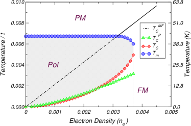
Figure 4: Phase boundaries obtained within the IPM. The polaronic phase (Pol) appears as a precursor to the ferromagnetism (FM) at low densities (dashed region). The dotted-line curve represents $T_{C}$ obtained in mean field. See the text for other notations. The left vertical scale is in units of $t$, and the one on the right in Kelvin, using $t=0.55$ eV.

As discussed above, in the present framework the $\textrm{PM}\rightarrow\textrm{Pol}$ transition in this diagram is of first order and, strictly speaking, the same occurs at the $\textrm{Pol}\rightarrow\textrm{FM}$ transition, because the phase boundaries are calculated from the relative stability of the two phases. At first sight this would mean that, during the $\textrm{Pol}\rightarrow\textrm{FM}$ transition, the magnetization has a discontinuity at $T_{C}$. However, from the interpretation of the FM transition in terms of polaron percolation, one expects a continuous transition, in the sense that the magnetization of the system should be weighted by the mass of the infinite percolating cluster, which evolves continuously from the percolation threshold. Finally, it is interesting to notice the order of magnitude of the relevant temperatures and densities for this phase. If, for definiteness, one assumes that $t\sim 1\,\textrm{eV}$, eqs. (9) and (11) reveal that the stability condition is realized for densities of $\sim 10^{-3}$, and temperatures typically in the dozens of Kelvin. As is shown in Appendix A, a more realistic approximation for the electronic energy doesn’t appear to modify these ranges significantly, which somehow restrict the range of materials where the effect might be realizable.

IV Polaronic Evidence in EuB${}_{\text{6}}$

As mentioned earlier, $\mathrm{EuB_{6}}$ is a magnetic metal with extremely reduced electron density, and exhibits all the characteristic signatures of a polaronic phase in Raman scattering measurements Nyhus et al. (1997); Snow et al. (2001). Such experiments reveal that the FM transition at $T_{C}\simeq 15$ K is preceded by an interval of temperatures where the response of the system is dominated by the presence of magnetic polarons.

It has been proposed in LABEL:~V. M. Pereiraet al., 2004 that $\mathrm{EuB_{6}}$ is very likely a DEM material in the low density regime, characterized by a hopping integral of $t=0.55\,\textrm{eV}$, and a carrier density per unit cell $n_{e}\sim 3\times 10^{-3}$. Subsequent magneto-optical experiments tally with this DE-based interpretation Caimi et al. (2006).

If we incorporate such hopping (found to reproduce the variation in $\omega_{\text{p}}$ for $\mathrm{EuB_{6}}$) in the phase diagram for the independent polaron model, the result is the one shown in Fig. 4, where the absolute temperatures should be read in the right vertical axis. It is interesting to compare this phase diagram for $n_{e}\simeq 0.003$ with the experimental evidence from the spin-flip Raman scattering results of LABEL:~Nyhus et al., 1997. The experiment reveals a polaronic region being stabilized essentially in the same temperature range as the one in Fig. 4 for the appropriate densities. This seems to show that our simple description of the polaronic phase captures the essential details of the polaron physics in $\mathrm{EuB_{6}}$. In particular, we emphasize that, the calculation of the Curie temperature based on the de Gennes approach (the dotted portion of the straight line in Fig. 4), clearly overestimates the actual $T_{C}$ by a factor of 3 or more inside the polaron stability range. As a matter of fact, placing ourselves at a density $n_{e}=0.003$ in the diagram of Fig. 4, we find $T_{C}\simeq 17$ K. This lies noticeably close to the experimental $T_{\text{C}}$, without adjusting parameters.

V The Problem of Phase Separation

The independent polaron model discussed before, is based on various approximations that stem from the low electronic density of the systems we aim to describe. In particular, the same assumption for the electronic energies used by de Gennes was employed. One of the implications of approximating eq. (4) by $E_{el}(M,n_{e})\approx E_{b}(M)n_{e}$ is that the Curie temperature calculated in mean-field for homogeneous PM and FM phases is simply proportional to the electronic density. This happens because the electronic density, $n_{e}$, appears together with the only energy scale in the problem, $t$.

But a more serious question regarding the double exchange in the low density limit is the problem of phase separation (PS). It is know that the DEM is unstable towards phase separation at low carrier densities, even without additional AFM (superexchange) couplings between the lattice spins Nagaev (1998); Yunoki et al. (1998); Arovas et al. (1999); Kagan et al. (1999); Alonso et al. (2001a, b). In order to study this aspect of the model in more detail, we will abandon the previous single particle approximation for the electronic energy, and calculate this quantity exactly within a hybrid thermodynamic approach (HTA) discussed next.

V.1 Hybrid Thermodynamic Approach

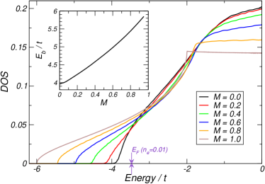
Figure 5: Numerical DOS for the DEM at different magnetizations, as defined in eq. (21). The arrows signal the position of $E_{F}(\mathcal{M}=0)$ for an electron concentration of $n_{e}=0.01$. The inset is a plot of the band edge as a function of the local magnetization.

The DE Hamiltonian (2) represents a system of classical spins that do not interact directly via a conventional exchange term. Their interaction comes indirectly from the fact that certain configurations of the local spins will minimize the energy of the electron gas. At absolute zero temperature, it is more or less evident that the ground state corresponds to ferromagnetism for any density of electrons Tsunetsugu et al. (1997). For other than this specific case, thermodynamics comes into play. All relevant quantities follow from the partition function

$$\Xi=\int\mathcal{D}\vec{S}_{i}\,\operatorname{Tr}\Bigl{[}\exp\bigl{(}-\beta(\mathcal{H}(\vec{S}_{i}\,)-\mu N)\bigr{)}\Bigr{]}\,.$$ (12)

The integral spans all local spins, $\vec{S}_{i}\,$, and the trace is over the electronic degrees of freedom, for which $N$ is the number operator. The electrons can be easily traced out in this grand canonical ensemble yielding an (exact) effective spin Hamiltonian that reads

$$\Xi=\int\mathcal{D}\vec{S}_{i}\,\exp\bigl{(}-\beta H_{eff}(\vec{S}_{i}\,)\bigr{)}\,,$$ (13)

with

$$\beta H_{eff}=-\sum_{n}\log\Bigl{[}1+\exp\bigl{(}-\beta(E_{n}(\vec{S}_{i}\,)-\mu)\bigr{)}\Bigr{]}\,,$$ (14)

$E_{n}(\vec{S}_{i}\,)$ being the eigenenergies of the one-electron Hamiltonian. Here, however, lies the origin of the difficulties that this system poses to analytical and numerical approaches. The latter are rather notorious, for one might think that once the effective spin Hamiltonian is written down, the energy of spin configurations can be calculated and the problem can be tackled with usual Monte Carlo (MC) techniques. That is indeed so formally. Unfortunately, the effective Hamiltonian — that is, the energy associated with a given spin configuration — requires the knowledge of the electronic eigenstates associated with such configuration. In other terms, the MC methodology would imply the full re-diagonalization of the electronic problem at every tentative update of the local spin configuration. This is clearly prohibitive, imposing an upper limit of $\sim 6^{3}$ to $8^{3}$ on the sizes of the systems that can be thus studied Calderón and Brey (1998); Dagotto (2003).

Our approach to this problem tries to circumvent these issues through a compromise in which the electronic problem is solved exactly and the spin subsystem treated within mean-field Alonso et al. (2001a). It hinges upon the fact that, writing $H_{eff}$ in terms of the total electronic DOS

$$\beta H_{eff}=-\int_{-\infty}^{\infty}\rho(E,\vec{S}_{i}\,)\log\Bigl{[}1+\exp\bigl{(}-\beta(E-\mu)\bigr{)}\Bigr{]}dE\,,$$ (15)

the dependence on the spin configuration is completely transferred to the DOS. Since the treatment of the exact effective Hamiltonian is out of reach, we resort to the Bogoliubov-Gibbs inequality for the canonical free energy:

$$\mathcal{F}\equiv-T\log(\Xi)\leq\left\langle H_{eff}\right\rangle_{t}-T\mathcal{S}_{t}\,.$$ (16)

Here $\left\langle...\right\rangle_{t}$ means the averages are calculated with a trial statistical operator — other than the canonical Maxwell distribution — and $\mathcal{S}_{t}$ is the associated entropy. Since our system is expected to exhibit either ferro or paramagnetism, the simplest suitable choice is the one generated by the uniform mean-field Hamiltonian

$$\mathcal{H}_{t}=-h\sum_{i}^{N}\vec{S}_{i}\,^{z}\,,$$ (17)

where $h$ is a variational parameter used to minimize the inequality (16). Since all averages are now done with regard to this $\mathcal{H}_{t}$, we have:

$$M\equiv\left\langle\vec{S}_{i}\,\right\rangle_{t} =\int\mathcal{D}\vec{S}_{i}\,\exp(-\beta\mathcal{H}_{t})\vec{S}_{i}\,$$

$$=\left(\coth(\beta h)-\frac{1}{\beta h}\right)\,\vec{u}_{z}$$

$$=\mathcal{L}(\beta h)\,\vec{u}_{z}\,,$$ (18)

where $\mathcal{L}(x)$ is the familiar Langevin function,

$$-T\mathcal{S}_{t}=\log\left[\frac{\sinh(h)}{h}\right]-hM\,,$$ (19)

and

$$\beta\left\langle H_{eff}\right\rangle_{t}=-\int_{-\infty}^{\infty}\left\langle\rho(E,\vec{S}_{i}\,)\right\rangle_{t}\log\Bigl{[}1+\exp\bigl{(}-\beta(E-\mu)\bigr{)}\Bigr{]}dE\,.$$ (20)

Therefore, the trouble in calculating the equilibrium free energy now boils down to the computation of $\bigl{\langle}\rho(E,\vec{S}_{i}\,)\bigr{\rangle}_{t}$. We know Haydock et al. (1972, 1975); Pereira (2006) that the recursive method can be used to obtain the exact $\rho(E,\vec{S}_{i}\,)$ for a given configuration $\{\vec{S}_{i}\,\}$. It is then a matter of straightforward statistics to obtain the averaged DOS. Hence, the electronic problem is still treated exactly for every configuration of local spins. These configurations are generated with the probability distribution $\sim\exp(-\beta h\sum_{i}\vec{S}_{i}\,^{z})$ and, since $\beta h$ and $\mathcal{M}$ are univocally related through (18), we simplify the notation and write

$$\bigl{\langle}\rho(E,\vec{S}_{i}\,)\bigr{\rangle}_{t}\equiv\rho(E,M)$$ (21)

whenever we refer to the DOS averaged over configurations of disorder compatible with an average magnetization $M$.

We also recall that when $E_{F}\gg T$, the logarithm in Eq. (20) can be replaced by $\Theta(\mu-E)$ meaning that the thermal excitations of the electronic subsystem can be neglected to a great extent. According to our earlier discussion, we are interested in cases for which $t\sim 1$ eV and $T_{\text{C}}\ll t$. This suggests a “zero-temperature” description of the electronic system, the thermal/entropic effects being assigned entirely to the spin subsystem End (b).

V.2 Canonical Free Energy and PhaseDiagram

Unless whenever stated otherwise, throughout this section we will be concerned only with the homogeneous phases (PM and FM) of the DEM. In the HTA one tries to trace the electrons out of the problem and obtain an effective Hamiltonian for the lattice spins, in such a way that the partition function becomes simply (14):

$$\Xi=\int\mathcal{D}\vec{S}_{i}\,\exp\bigl{(}-\beta H_{eff}(\vec{S}_{i}\,)\bigr{)}\,.$$

This effective Hamiltonian contributes to the total free energy through eqs. (16), (19) and (20), and we have, at the end:

$$\mathcal{F}(M,n_{e})=\int^{E_{F}(n_{e},M)}\epsilon\rho(\epsilon,M)d\epsilon-T\mathcal{S}(M)\,.$$ (22)

The free energy in eq. (22) should be minimized with respect to $M$ to obtain the equilibrium free energy $\mathcal{F}_{eq}(n_{e})$. We work at constant electron density and our focus in the cases where $T\ll t$ is implicitly assumed in the omission of the electronic entropy. The phase diagram that emerges from the minimization of (22) is drawn in Fig. 6 and reproduces End (c) the results obtained by LABEL:~Alonso et al., 2001a.

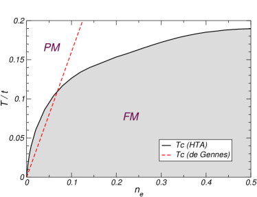
Figure 6: Phase diagram of the DEM obtained within the HTA. For comparison, the result for $T_{C}$ obtained by de Gennes is also plotted (dashed line) [cfr. LABEL:~Alonso et al., 2001a].

The PM–FM transition happens to be continuous for all densities and the deviations from the result obtained with the bottom of the band, de Gennes-like, approximation are quite evident. It turns out, however, that this phase diagram is incomplete.

V.3 The Essence of the Problem

Reflecting the relative stability of the two homogeneous phases, the plot in Fig. 6 says nothing regarding density fluctuations. To determine whether the system is unstable in relation to density fluctuations, we need to look at the behavior of the equilibrium free energy, $\mathcal{F}_{eq}(n_{e})$, namely its dependence on the electronic density.

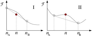
Figure 7: Free energy for a system unstable towards density fluctuations. The system is unstable for $n_{A}<n<n_{B}$ and segregates between regions of density $n_{A}$ and $n_{B}$. The Maxwell construction restoring the curvature of $\mathcal{F}_{eq}(n_{e})$ is represented by the dashed lines.

Thermodynamic stability requires $\mathcal{F}_{eq}(n_{e})$ to be a globally upward convex function, so that the compressibility, $\kappa=n^{-1}\partial n/\partial\mu$, is never negative. Whenever this condition is violated and the density of the total system is kept constant, it will naturally segregate into two distinct phases in such a way that guarantees the restoration of convexity in the resulting free energy. The equilibrium state in this phase-separated region can be obtained by the so-called Maxwell construction, which, geometrically, is tantamount to substituting the underlying $\mathcal{F}_{eq}(n_{e})$ by the envelope of all inferior tangents Callen (1985). A sketch of the situation is presented in Fig. 7.

It so happens that, when the behavior of the isothermals of $\mathcal{F}_{eq}(n_{e})$ for the DEM calculated using eq. (22) is analyzed, the signature of this instability emerges at low densities by the violation of the global convexity. A typical result is shown in detail in Fig. 8.

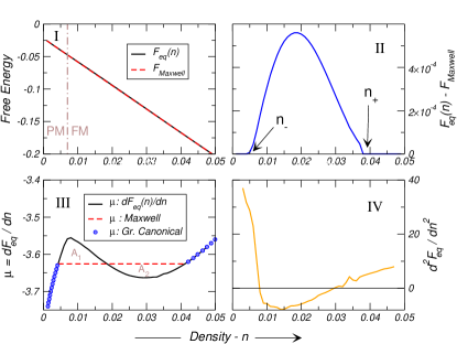
Figure 8: Details of the Maxwell construction for the DEM at $T=0.03t$ . The result of the construction is barely discernible from the underlying $\mathcal{F}_{eq}(n_{e})$ (I) and, for clarity their difference is plotted on panel II. For comparison, the chemical potential extracted from the results in I is shown together with calculations in the grand canonical ensemble (III). Panel IV shows $\partial^{2}\mathcal{F}_{eq}/\partial n_{e}^{2}$ .

Since there is a considerable amount of information in this figure let us go through it in detail (everything is calculated at a constant temperature, $T=0.03t$).

In the first panel (I) we show the equilibrium free energy $\mathcal{F}_{eq}(n_{e})$ as a function of the electronic density $n_{e}$ (continuous/black line). Despite looking like a straight line, it does have a slight upwards curvature at the lowest densities, downwards at intermediate densities, and upwards again at higher densities. This can be seen in the curve $\partial^{2}\mathcal{F}_{eq}/\partial n_{e}^{2}$ plotted in panel (IV). Thus, we have an instability and a Maxwell construction has to be done in order to find the true equilibrium free energy of the system. The Maxwell construction is the dashed/red line in panel (I). Since the effect is rather subtle, we plot the difference between $\mathcal{F}_{eq}(n_{e})$ and the free energy after the Maxwell construction in panel (II). In panel (I) we also show the density corresponding to the PM–FM transition at this temperature, signaled by the dot-dashed vertical line (cfr. Fig. 6). If we call this particular density $n_{e}(T_{C}=0.03)$, then it is clear that $n_{-}<n_{e}(T_{C}=0.03)<n_{+}$. Then, although the relative difference between the free energies is only $\sim 1\%$, it is qualitatively significant because the system exibiths coexistence of PM and FM, each of the coexisting thermodynamic phases having its own electron density.

In panel (III) we present the chemical potential calculated in three different ways. The first one (black/continuous) is simply the curve corresponding to $\partial F_{eq}(n)/\partial n$, and the instability is also clearly seen here since $\mu(n)$ should be monotonously increasing. The dashed (red) curve is the chemical potential resulting from the free energy after the Maxwell construction. Below $n_{-}$ and above $n_{+}$ the result is the same, but in between it is simply an horizontal line. Altough not shown in the figure, the position of this horizontal part is such that the areas $A_{1}$ and $A_{2}$ are exactly equal, as it should happen End (d). The third curve (circles) shows the chemical potential obtained my minimizing the free energy in the grand canonical ensemble. In this case, since not $n$ but $\mu$ is kept constant, the phase separation instability arises naturally through a discontinuity in the $\mu(n)$ curve. The discontinuity appears precisely in the region of densities where the Maxwell construction is in effect, and is just another way to observe this phenomenon.

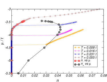
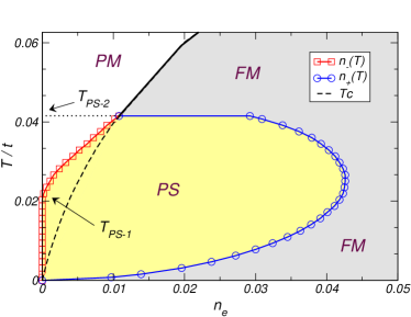
Figure 9: 9 Isothermals in the $\mu-n_{e}$ plane for selected temperatures. The coexistence curves $n_{-}$ (squares) and $n_{+}$ (circles) were obtained from the Maxwell construction, whereas the $\mu(n_{e})$ curves are calculated in the grand canonical ensemble, for comparison. 9 Detail of the low density region of the updated $T-n_{e}$ phase diagram. The phase separated region (PS) is bounded by the curves $n_{-}(T)$ and $n_{+}(T)$ obtained from the Maxwell construction.

Actually it is quite instructive to pursue in some more detail this complementarity between the canonical and grand canonical treatments for this particular case. Our scenario is completely analogous to the well known behavior of the van der Waals isothermals for the liquid–gas transition Callen (1985). This is best understood with reference to the plots of $\mu(n_{e})$ in Fig. 9 at several temperatures. Just as in the $P-v$ phase diagram of the gas, the $\mu(n_{e})$ curve is monotonous for temperatures above some critical value. Below this point, the compressibility of the system ($dn_{e}/d\mu$) becomes negative in some density interval implying an instability. The coexistence curve is then defined by $n_{-}$ and $n_{+}$ obtained from the Maxwell construction and, naturally, coincides with the jump in the density obtained in the grand canonical calculation. Despite the analogy and resemblance of the coexistence curve for the DEM and the van der Waals gas, there is an important qualitative detail not present in the latter case: the coexistence curve for the DEM is re-entrant.

The stability analysis was performed for all the temperatures and densities shown in the phase diagram of Fig. 6. The system is unstable towards phase separation at low densities, and the qualitative behavior of the thermodynamic functions is always the one discussed above. As a consequence, one obtains the updated phase diagram presented in Fig. 9.

The information conveyed by this diagram can be translated as follows: for densities above $n_{e}\sim 0.04$, the system is homogeneous and exhibits a magnetic transition at $T_{C}(n_{e})$. If the density is lower than $n_{e}\sim 0.01$ the system is homogeneous and PM at high temperatures until $n_{-}(T)$ is reached. At that point the homogeneous phase is no longer sustainable and two phases start to coexist: one with density $n_{-}(T)$ and PM together with another of density $n_{+}(T)$ and FM. Below a temperature signaled as $T_{\textrm{PS-1}}$, $n_{-}(T)=0$ and thus the PM portion of the system is devoid of electrons End (e). If $0.01\lesssim n_{e}\lesssim 0.04$, the re-entrant nature of the coexistence curve means that the system can become an homogeneous ferromagnet below $T_{C}(n_{e})$ but still segregate at lower temperatures whenever the condition $n_{e}=n_{+}(T)$ is met. In any case, the magnetization of the system is always continuous – a simple consequence of the relation between the densities and volume fractions of each phase:

$$n_{e}=n_{-}\frac{V_{-}}{V}+n_{+}\frac{V_{+}}{V}\,.$$ (23)

This constraint introduces some peculiarities regarding the nature of the phase separated state. To understand that, in Fig. 10 we draw a sketch of the phase separated region in the phase diagram of Fig. 9.

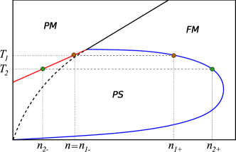
Figure 10: Schematic representation of Fig. 9.

Using this sketch as reference, assume that our system is initially at some high temperature $T>T_{1}$ and has a given density $n$. Under these circumstances, the phase diagram states that the equilibrium corresponds to an homogeneous PM phase. We can lower the temperature until $T_{1}$ is reached, at which point an instability arises. Exactly at $T=T_{1}$ there will be a segregation between a PM phase with density $n_{\textrm{1-}}=n$ and another, FM, with density $n_{1+}$. In order to satisfy the constraint (23), the volume fraction of the FM phase will be $V_{\textrm{1+}}=0$, at $T=T_{1}$. A slight decrease in the temperature from $T_{1}$ to $T_{2}$ will reorganize the system so that the PM phase with density $n_{\textrm{2-}}$ now coexists with a FM phase of density $n_{\textrm{2+}}$. For $T_{2}$ very close to $T_{1}$, the density of the PM phase is just slightly different from the global density:

$$n_{\textrm{2--}}=n-\varepsilon\,,$$ (24)

where $\varepsilon$ is a small quantity. This determines the volume fractions to be

$$V_{\textrm{2+}}\approx\frac{\varepsilon}{n_{\textrm{2+}}-n}\,.$$ (25)

Evidently, this means that most of the electrons still remain in the PM phase, and just a few populate the FM regions. But this poses a problem. The Coulomb interaction will certainly prevent the accumulation of charges in a very small volume and the system must remain neutral.

V.4 Electrostatic Suppression of Phase Separation

The Maxwell construction is inexpressive with regards to the spatial organization of the phase separated state. This follows from the fact that the Maxwell construction for two coexisting phases of densities $n_{+}$ and $n_{-}$ amounts formally to saying that,

$$\mathcal{F}_{\text{Maxwell}}(n)=\mathcal{F}(n_{+})\frac{V+}{V}+\mathcal{F}(n_{-})\frac{V-}{V}=\mathcal{F}(n_{+})x+\mathcal{F}(n_{-})(1-x)\,,$$ (26)

where $x=V_{+}/V$ and $V_{-}/V$ represents the volume fraction of the two coexisting phases. This is simply a linear interpolation between the two values $F(n_{+})$ and $F(n_{-})$, as illustrated in Fig. 7. Therefore, the resulting free energy, $\mathcal{F}_{\text{Maxwell}}$, corresponds to the situation where we have a system made of two independent thermodynamic components. In particular, the Maxwell prescription above says nothing about the way the system reorganizes when it phase-separates. This can only come from additional interaction terms that should be added to the right hand side of eq. (26), in order to include interaction, surface, boundary and perhaps other relevant effects or correlations. In our case the two phases have different electronic densities, both different from the homogeneous density, the latter satisfying

$$n=n_{+}x+n_{-}(1-x)\,.$$ (27)

Obviously, with mobile negative charges, the system can indeed adjust itself by accumulating electrons in some regions, and depleting them from others. But since the background of positive atomic charges stays essentially immutable and homogeneous, this means that the total charge of each phase is not zero. Coulomb interactions are therefore crucial. Under this assumption we now investigate two important corrections for the free energy in the phase separated regime.

V.4.1 Electrostatic Correction

Given that we are not assuming any sort of anisotropy, the electrostatic constraint will most certainly favor the development of bubbles of the FM, high density phase, dispersed in the PM, low density phase. Such scenario is schematically depicted in Fig. 11.

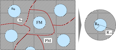
Figure 11: Depiction of the Wigner-Seitz construction discussed in the text. Each cell is replaced by an effective spherical cell characterized by the same densities.

The charge density is assumed uniform and continuous inside each FM bubble and across the PM background. To calculate the electrostatic energy associated with this charge distribution we take notice to the fact that, on the grounds of overall charge neutrality, it should be possible to find an appropriate neighborhood around each FM bubble such that the total charge on the bubble plus PM neighborhood adds to zero. In Fig. 11 this is represented by the wavy lines that, in this way, define cells of charge neutrality. Following Wigner Pines (1963), these cells are replaced by the equivalent Wigner-Seitz (WS) spherical cell containing the same volume fractions of FM and PM phases (as shown on the right-hand side of the diagram), which means that

$$R_{+}^{3}=xR_{-}^{3}$$ (28)

For each WS cell, the total electrostatic energy is calculated considering three terms

$$E_{C}=U_{++}+U_{--}+U{+-}\,,$$ (29)

with the first accounting for the electrostatic self-energy of the “+” region, the second the self-energy of the “-” region, and the last the mutual electrostatic interaction between the two. All of them are calculated within classical electrostatic theory assuming uniform charge distributions in the two regions. Hence

$$U_{++}=\frac{3}{5}\frac{Q_{+}^{2}}{R_{+}}\,,$$ (30)

and represents the electrostatic energy of the inner sphere containing the “+” region;

$$U_{--}=\frac{3Q_{-}^{2}}{R_{-}^{3}-R_{+}^{3}}\left(\frac{R_{-}^{5}-R_{+}^{5}}{5}-R_{+}^{3}\frac{R_{-}^{2}-R_{+}^{2}}{2}\right)$$ (31)

stands for the energy of the outer shell of the “-” region, and

$$U_{+-}=\frac{3}{2}Q_{+}Q_{-}\frac{R_{-}^{2}-R_{+}^{2}}{R_{-}^{3}-R_{+}^{3}}$$ (32)

is the electrostatic interaction between the inner sphere and outer shell. In the above $Q_{\pm}$ are the total charges (positive background + electrons) inside the two regions, and $R_{\pm}$ the respective radii, as depicted in Fig. 11. For reasons regarding numerical stability, in the following we will take always $n_{-}=0$. Looking at Fig. 9, this comes as a natural approximation because $n_{+}\gg n_{-}$ for $T_{PS1}<T<T_{PS2}$, and becomes exact for $T<T_{PS1}$. Hence, using the identities

$$Q_{+} =e(n-n_{+})V_{+}=en(x-1)V$$

$$V_{+} =\frac{4\pi}{3}R_{+}^{3}$$

$$Q_{-} =e(n-n_{-})V_{-}=en(1-x)V$$

$$V_{-} =\frac{4\pi}{3}(R_{-}^{3}-R_{+}^{3})\,$$ (33)

the Coulomb term can be cast as

$$E_{C}=\frac{8}{15}e^{2}\pi^{2}n^{2}R_{+}^{5}\frac{2-3x^{1/3}+x}{x^{2}}\,,$$ (34)

which yields an energy per unit of volume of

$$\epsilon_{C}=\frac{E_{C}}{V}=\frac{2}{5}\,e^{2}\,n^{2}\,\pi\,R^{2}\,\frac{2-3\,x^{1/3}+x}{x}\,.$$ (35)

For simplicity we replaced $R_{+}$ by $R$ and keep this lighter notation below. The bubble radius, $R$, is a variational parameter. The result (35) implies that, for a given volume fraction of the two phases, say $x$, the electrostatically favorable situation is to shrink the FM bubbles to an arbitrarily small size, meaning that $R\to 0$ End (f). But this treatment is yet incomplete, inasmuch as the consideration of finite-sized bubbles of electrons requires another correction, of different nature, to the ground-state energy.

V.4.2 Phase Space Correction

The electronic contribution to the free energy (22) is calculated in the thermodynamic limit. In the phase separated regime, the electron rich bubbles are expected to be of relatively small size. Therefore, one cannot rely on the electronic energy calculated in the thermodynamic limit and the need to introduce finite size corrections arises.

The leading correction to the energy of an electron gas confined to a finite sized volume comes through the correction to the electronic DOS of the free electron gas which, as discussed in Appendix B, leads to a correction to the ground state energy per electron reading

$$\frac{E(R,n_{+})}{N_{e}}=\frac{E(\infty,n_{+})}{N_{e}}\left[1+\frac{15}{16}\left(\frac{\pi}{6n_{+}}\right)^{1/3}\frac{1}{R}\right]\,.$$ (36)

The term in $R^{-1}$ is the correction for each bubble. To obtain the total correction we just multiply by the number of WS cells, obtaining the total energy per unit volume

$$\frac{E(R,n_{+},x)}{V}=\frac{E(\infty,n_{+})}{V}\left[1+\frac{15}{16}\left(\frac{\pi}{6n}\right)^{1/3}\frac{x^{1/3}}{R}\right]x\,.$$ (37)

As expected, the phase space correction acts to the effect of rising the ground state energy of the electron gas. This induces a tendency opposed to the one embodied in the electrostatic term (35), and the two should balance at some optimum value of $R$.

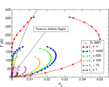
Figure 12: Phase diagram calculated within the HTA with a corrected Maxwell construction according to eq. (38). The arrow marks the polaronic stability region, represented by the dashed area at low density and temperature. Notice how the region of phase separation lies inside the polaronic bubble for dielectric constants of $\varepsilon_{r}\sim 1$.

The free energy in the phase separated regime (26) needs to be updated for these two corrections that go beyond the Maxwell construction. The result is

$$\mathcal{F}_{Maxwell}(n)=\mathcal{F}(n_{+})x+\mathcal{F}(n_{-})(1-x)+\frac{2}{5}\,e^{2}\,n^{2}\,\pi\,R^{2}\,\frac{2-3\,x^{1/3}+x}{x}+\frac{E_{el}(n_{+})}{V}\frac{15}{16}\left(\frac{\pi}{6n}\right)^{1/3}\frac{x^{4/3}}{R}\,.$$ (38)

Since the FM radius is entering only in the correcting terms, the minimization with respect to $R$ can be performed at once, and the final result is

$$\mathcal{F}_{Maxwell}(n)=\mathcal{F}(n_{+})x+\mathcal{F}(n_{-})(1-x)+\frac{3}{2^{2/3}}\left(\frac{2}{5}\frac{e^{2}}{a}\pi n_{e}^{2}\right)^{1/3}\left[\frac{3}{5}\,t\,n_{e}(6\pi^{2}n_{e})^{2/3}\frac{15}{16}\left(\frac{\pi}{6n_{e}}\right)^{1/3}\right]^{2/3}\left[\frac{2+x-3x^{1/3}}{x^{5/3}}\right]^{1/3}\,.$$ (39)

This last expression is the free energy per site of the original lattice when phase separation is in effect. $a$ is the lattice parameter, $n_{e}$ the electron density per unit cell of the crystal, and $t$ is the hopping integral. Naturally, when there is no PS instability, $x=1$ by definition and the above reduces to $\mathcal{F}(n_{e})$ as one certainly expects. In the PS regime, the equilibrium radius of the electron rich FM bubbles satisfies

$$\frac{4}{3}\,\pi\,n_{+}R^{3}=\dfrac{15}{16}\frac{at}{e^{2}}\left(\frac{6\pi^{5}n_{e}}{x}\right)^{1/3}\frac{1}{2+x-3x^{1/3}}\,,$$ (40)

and this relation can be used, for instance, to inspect the typical number of electrons inside each FM bubble.

V.5 Consequences for the Phase Diagram

The natural question is now: what happens when the equilibrium free energy is recalculated with these corrections? Namely, we want to know wheather the PS instability persists when the Maxwell construction is updated according to (39). It is useful to have a tuning parameter that interpolates between the case in (39) and the previous calculation where electrostatic and localization effects were disregarded. With that purpose, we introduce the dielectric constant, $\varepsilon_{r}$, that renormalizes the electron charge as $e^{2}\to e^{2}/\varepsilon_{r}$ in the expressions above. By varying $\varepsilon_{r}$ between $1$ and $1000$ the curves in Fig. 12 were obtained. In this plot, we are focusing on the low density region of the phase diagram where PS occurs. The red (circles) curve pertains to the case $\varepsilon_{r}\to\infty$ (or, equivalently, zero electronic charge) and is again the result shown before in the phase diagram of Fig. 9 End (g). The figure is transparent as to what happens when the Coulomb interaction is turned on: the PS region is progressively reduced! Not only that but it is clear that an overwhelming shrinking of the PS region takes place when $\varepsilon=1$, which is a reasonable value, considering the low electronic densities.

Thus, the consideration of the free energy (39), corrected for the effects arising as a consequence of charge accumulation, leads to the suppression of the PS instability. The electrostatic payoff involved in the segregation leads the system to phase-separate only at much lower densities and/or temperatures. Just how low these are is controlled by the effective electronic charge.

V.6 Phase Separation and Magnetic Polarons

There is a question of relevance that we have been postponing since the beginning of this section on the problem of PS. In Sec. IV calculated the phase diagram of Fig. 4 describing the stability conditions for free magnetic polarons in the DEM. From the polaronic phase diagram follows that magnetic polarons are only stable at considerably low temperatures and densities. In fact much lower than the temperatures and densities at which the PS instability sets in. The reader might have noticed since Fig. 10 that the density and temperature scales for the PS bubble are much higher than the scales for the polaronic bubble. More precisely, the polaronic phase lies well inside the PS region when the corrections to the Maxwell construction are ignored. These two regions can be seen in perspective in Fig. 12, where the polaronic stability region is highlighted by the dashed region in the lower left corner, and completely inside the PS region for $\varepsilon\to\infty$.

This is clearly a problem to our arguments concerning the polaronic phase. The polaronic stability has been determined by studying its relative stability with regards to an homogeneous FM phase. The diagram above is saying that, at such low densities, there are no homogeneous phases — the system phase separates! So the study of polaronic stability has a problem.

But this is only if the electrostatic effects are ignored.

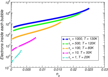
Figure 13: The number of carriers inside each FM bubble calculated according to (40) for selected temperatures and dielectric constants.

With their inclusion, the PS region retreats to lower and lower densities and, as the figure documents, for $\varepsilon_{r}\sim 1$, it rests already completely inside the polaronic region. So, it seems that the problems above with the polaronic phase have just diminished.

The connection between PS and magnetic polarons is indeed remarkably close. The ferromagnetic droplets, associated with a localization energy for the electrons in a restricted volume, are nothing more than our description of the magnetic polaron. So, in this sense, the PS regime studied here and the magnetic polarons are different perspectives of the same physical concept. One of the differences is that, while the magnetic polaron is defined as a FM droplet with a single electron, the PS regime allows for droplets with many electrons.

To explore this further, it is interesting to know the number of electrons inside each FM bubble in the PS regime. Some typical results are plotted in Fig. 13 for the same $\varepsilon_{r}$ used before. The most remarkable fact about these curves is that the one pertaining to $\varepsilon_{r}=1$ is of the order of unity. Therefore, there is essentially one electron per FM droplet. In addition, the temperatures at which PS occurs for this value of $\varepsilon_{r}$ are so low that the FM droplets are very nearly full polarization. But, a fully polarized FM droplet with one electron inside is just our definition of magnetic polaron! Thus, the peculiarities of the phase segregation in this system are completely consistent with the magnetic polaron picture and, with that respect, the similarity between the shape of the two phase diagrams (Figs. 9 and 16) seems hardly coincidental.

V.7 General Argument Regarding Phase Separation

Although we have been focusing so far on the specificities of the phase separation instability in the DEM, phase separation is quite a general phenomenon in thermodynamics. To conclude our discussion we put forward an argument showing that, if the contribution of the entropy of the electronic gas can be neglected in the total free energy, then phase separation is ubiquitous in electronic systems whose bandwidth is magnetization dependent. To see how this comes about, recall that the free energy (22) is given by only two contributions: the electronic ground state energy plus an entropic term attributed uniquely to the local moments. For reasons that will be clear in a moment, this argument unfolds more clearly if we work in the grand canonical ensemble, where the electronic chemical potential, $\mu$, is held constant. In this case the free energy (22) is simply replaced by the grand canonical potential, and is akin to replacing $E_{F}\rightarrow\mu$ and $\varepsilon\rightarrow\varepsilon-\mu$ there.

Consider now the following facts, regarding the relevant thermodynamic quantities seen as functions of the magnetization:

1. The magnetic entropy (19) is monotonous and downward convex, for all the domain of $M$;

2. For a given chemical potential, $\mu$, the electronic energy is monotonous and downward convex throughout the entire domain of variation of $M$;

3. The electronic density is monotonous and upward convex.

Statement 1 follows from the fact that $\mathcal{S}(M)$ is a proper thermodynamic entropy for a magnetic system, having all the required analytical properties.

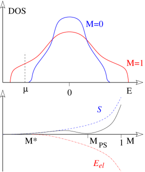
Figure 14: Schematic variation of DOS, entropy and electronic energy with $M$ at constant $\mu$. In the top panel we illustrate the changes in the DOS with increasing magnetization, and the corresponding increase in bandwidth. In the lower panel we illustrate the variation of the electronic energy and magnetic entropy, and how they combine to yield the free energy depicted by the black (solid) line.

Point 3 is a trivial consequence of the electronic density being the integrated DOS. Point 2 can be understood from the fact that the electronic bandwidth is monotonous with $M$ (cfr. Fig. 5). There is a subtlety however in that, if $\mu$ happens to be below the band edge at $M=0$, then, the electronic energy will be identically zero until some critical magnetization, say $M^{*}$, is reached for which the band edge coincides with $\mu$. For higher magnetizations, the energy decreases and the overall shape is as depicted in Fig. 14. Since the same plateau is present in the electronic density, for exactly the same reasons, the result for the grand canonical potential will be something like the solid curve drawn schematically in the bottom frame panel of Fig. 14. Evidently, there will be a temperature at which the minimum of this curve exactly touches the horizontal axis (as depicted), thus precipitating a first order transition. At the precise temperature, $T$, at which this happens, the system stays undecided as to which state it should have because the thermodynamic potentials at $M=0$ and $M=M_{PS}$ are degenerate. Since $\mu$ is kept constant, $M=0$ and $M=M_{PS}$ correspond to different electronic densities. This is but our phase separation instability seen from the grand canonical perspective.

The important thing here is that nothing in this argument mentions the details of the specific model under consideration, and therefore is valid as long as the basic assumptions remain valid. In particular, the magnetization is as good as any other suitable thermodynamic parameter, and, thus, the arguments extends to any appropriate classical variable coupled to the electronic energy as the magnetization is in our specific case.

That phase separation has to emerge always follows from the fact that one can always place $\mu$ in between the band edges at $M=0$ and $M=1$. So, if temperatures are so low that the fermionic entropy can be disregarded, this kind of treatment should always yield a phase separated regime at low densities.

VI The regime of ultra low densities

Having clarified the issue of phase separation and its connections with the polaronic phase, we return now to the polaronic description. The consideration of electron-electron interaction, as done in the previous section, amounts to effectively describing the electrons in terms of the Hamiltonian

$$\mathcal{H}_{DE} =-\sum_{\left\langle i,j\right\rangle}a_{ij}d_{i}^{{\dagger}}d_{j}+\textrm{h. c.}$$

$$+e^{2}\sum_{i>j}\frac{(n_{i}-n_{e})(n_{j}-n_{e})}{|{\bf r}_{i}-{\bf r}_{j}|}\,,$$ (41)

where the presence of the Coulomb term is now explicit. The presence of the full Coulomb interaction in Eq. (41) is to be understood in connection with the case of extremely reduced electron density. In a conventional Fermi liquid the high density of electrons makes the screening process very effective, and the effect of the electron-electron interactions can be absorbed into the renormalization of physical quantities such as the effective mass. In a very diluted electron gas the Coulomb interaction cannot be addressed meaningfully in this way. In the language of the one component plasma, this can be understood with reference to the dimensionless parameter $r_{s}=r_{o}/a_{0}$, where $r_{o}=(3/4\pi\rho)^{1/3}$ ($\rho$ being the volumetric density of electrons) is the average distance between electrons, and $a_{0}$ is the Bohr radius. While the kinetic energy scales as $1/r_{s}^{2}$, the potential energy varies as $1/r_{s}$, and, therefore dominates in the low density ($r_{s}\to\infty$) regime Pines (1963).

It is well known since Wigner Wigner and Seitz (1934) that, under such circumstances, the electrons arrange themselves in a regular lattice, and electron localization occurs. If a so-called Wigner crystal is realizable in a system described by Eq. (41) then, as in any solid, there is zero point motion of the electrons about their equilibrium positions. If the electron itinerates among several unit cells during this zero point motion, the magnetic coupling, $J_{H}$, leads to the local polarization of the lattice spins, producing a bound magnetic polaron and generating a polaronic Wigner crystal. This process is obviously limited by the melting of the electronic solid and, thus, the question arises of how to describe these two tendencies for the polaron formation and the interplay of Coulomb and magnetic interactions. We present estimates regarding the stability of this polaronic Wigner crystal below.

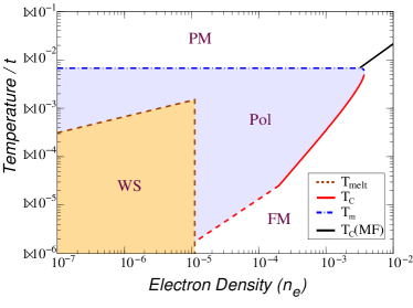
Figure 15: Phase diagram of the diluted DEM model as a function of temperature and density ($t=0.5\,\textrm{eV},a=4\,\textrm{\AA}$): paramagnetic (PM), polaronic (Pol), polaronic Wigner solid (WS), and ferromagnetic (FM). Notice that the axes are presented on a logarithmic scale (cfr. Fig. 4).

VI.1 Polaronic Wigner Crystal

Following the Wigner-Seitz approximation Pines (1963), the Wigner crystal unit cell (much larger than the original lattice spacing, $a$) is approximated by an electrically neutral spherical volume, inside which the ionic charge density is homogeneous. The electrostatic potential energy then depends only upon $r$: the distance of the electron from the center of the cell. The Hamiltonian for an electron in this uniform charge and spin background is then:

$$\mathcal{H}_{W}=-6t-\frac{3}{2}\frac{e^{2}}{r_{o}}+\frac{p^{2}}{2m}+\frac{1}{2}m(\omega_{e}^{2}+\omega^{2})r^{2}\,,$$ (42)

where $p$ is the electron momentum, $m=1/(2a^{2}t)$ the effective electron mass, and $\omega_{e}^{2}=\omega_{p}^{2}/3=e^{2}/mr_{o}^{3}$, where $\omega_{p}$ is the plasma frequency. In Eq. (42) $\omega$ is the frequency of the confining potential due to the DEM mechanism, and is a variational parameter. The radius of the magnetic polaron in the Wigner crystal relates to $\omega$ by:

$$R=\sqrt{3t/\Omega}\,,$$ (43)

where $\Omega=\sqrt{\omega_{e}^{2}+\omega^{2}}$ is the total frequency of oscillation of the electron. Notice that the ground state energy of Eq. (42) is $E_{0}=-6t-3e^{2}/(2r_{o})+3\Omega/2$ and hence the relative gain in free energy is:

$$\Delta\mathcal{F}_{WP}=-2t+3\left(\Omega-\omega_{e}\right)/2+4\pi R^{3}T\log\left(2S+1\right)/3.$$ (44)

Minimization of Eq. (44) with respect to $\omega$ gives:

$$R(T)=\left\{\begin{array}[]{c}\begin{array}[]{ll}R_{S}\,\,\left(T^{*}/T\right)^{1/5}&,T>T^{*}\\ R_{S}&,T\leq T^{*}\end{array}\end{array}\right.\,,$$ (45)

where $R_{S}=[3t/(\omega_{e})]^{1/2}$ is the saturation radius, and $T^{*}/t=9/[4\pi R_{S}^{5}\log\left(2S+1\right)]$ is the temperature below which the polaron radius saturates due to the interplay between the DEM and the Coulomb interaction.

VI.2 Wigner Crystal Melting

It is clear that the previous results are valid for temperatures so low as not to melt the Wigner solid. The calculations for the independent polaron model reveal that the temperatures for polaron stability are already typically small for reasonable values of $t$, but the electronic solid is much more sensitive to the temperature. The Wigner crystal melting temperature, $T_{M}$, can be estimated from the Lindemann’s criteria Jones and Ceperley (1996): $T_{M}\approx 0.01(e^{2}/a)n_{e}^{1/3}$. It is known from several numerical calculations Cândido et al. (2004); Ortiz et al. (1999); Jones and Ceperley (1996) on the stability of the one component plasma, that the maximum densities and temperatures at which the Wigner crystal can exist correspond to $r_{s}\sim 50\textrm{-}100$, and $T\sim 10\,\textrm{K}$. Values of $r_{s}\sim 50\textrm{-}100$ correspond to $n_{e}\sim 10^{-6}\textrm{-}10^{-5}$ for $t=1\,\textrm{eV}$ and $a=4\,\textrm{\AA}$. The region of stability of the polaronic crystal is show in Fig. 15. Due to the absence of magnetic interactions between different polarons, the Wigner crystal should be a superparamagnet: the local moments within the zero point radius of the electrons are expected to respond collectively. In the presence of other long-range interactions (such as dipole-dipole) the polaronic Wigner crystal can exhibit long range magnetic order. Increasing the electron density at $T=0$ causes the Wigner crystal to quantum melt at a critical density with two possible outcomes: a paramagnetic polaronic Fermi liquid or a fully polarized ferromagnet. In both cases the carriers are mobile and can screen the long-range part of the Coulomb interaction leading to a Fermi liquid state. At finite temperatures, where the electron state cannot be described by the zero point motions implicit in Eq. (42) alone, the crystal should follow the features of the phase diagram for the electron gas Jones and Ceperley (1996). The characterization of the system in the neighborhood of the melting point, where the presence of a polaron liquid is plausible [Fig. 15], is restrictively hard, even for the simple electron gas. Far from this region, where the electron density is high enough to make the screening process effective, one expects to retrieve the behavior obtained before within the independent polaron model, and discussed previously.

VII Conclusions

The pure double exchange model Hamiltonian (2) displays a rich phase diagram, even at the lowest densities. This is in itself noteworthy insofar as we did not introduce any additional competing interactions, such as direct magnetic couplings among the local spins. In addition to its intrinsic tendency for a FM transition at low temperatures, the low density region of the phase diagram displays an instability towards phase separation. This phase separated regime is characterized by FM droplets rich in electrons, embedded in a PM background, essentially depleted of electrons. The consideration of electron-electron interactions shows that, as expected, the phase separated regime is highly suppressed for meaningfull magnitudes of the electrostatic correction. This suppression is such that the effective number of electrons inside each FM droplet becomes of the order of unity. Given that, by construction, our WS cells containing the FM droplet are neutral, this situation of nearly one electron per droplet can be alternatively addressed in terms of non-interacting magnetic polarons.

This justifies our initial approach to address the polaronic phase in the low density double exchange model. Within the independent polaron model developed in Sec. III, below a critical density the PM-FM transition is mediated by a polaronic phase (cfr. Fig. 4). One consequence of this is that the Curie temperature of the system is much lower than one would obtain if based only on a PM-FM mean-field approximation. Moreover, by considering the model parameters already used in LABEL:~V. M. Pereiraet al., 2004 to describe other properties of $\mathrm{EuB_{6}}$ from a DE point of view, we obtain the range of temperatures $T_{m}<T<T_{\text{C}}$ for the presence of the polaronic phase in agreement with experimental observations, and without additional adjustable parameters.

Further down in the density scales we estimated the conditions for the stability of a polaronic Wigner crystal. This phase seems plausible in the ultra diluted situation where Wigner cristalization of the electron gas is expected. In this case the zero point motion of the electrons can still provide enough itinerancy to polarize the neighboring local moments, generating a crystal of bound magnetic polarons. Nevertheless this regime, although rather appealing from the theoretical point of view, is certainly difficult to reach experimentally on account of the reduced temperature and density scales involved.

The current results complement the ones in LABEL:~V. M. Pereiraet al., 2004 that pertain, mostly, to the evolution of the system once the homogeneous FM phases sets in, whereas now we have addressed how the transition from homogeneous PM to the onset of homogeneous FM takes place. We can then interpret the ferromagnetic transition in $\mathrm{EuB_{6}}$ as being precipitated by the merging of magnetic polarons which attain the percolation threshold close to $T_{\text{C}}$. At the same time, these results lend additional support to the interpretation of the phenomenology of $\mathrm{EuB_{6}}$ from a double exchange perspective.

VIII Acknowledgments

We acknowledge many motivating and fruitfull discussions with L. Degiorgi and E. V. Castro. V. M. Pereira is supported by Fundação para a Ciência e a Tecnologia via SFRH/BPD/27182/2006. V. M. Pereira and J. M. B. Lopes dos Santos further acknowledge POCI 2010 via the grant PTDC/FIS/64404/2006.

Appendix A Effects of Finite Band Filling on Polaron Stability

In the main discussion of the polaronic physics in the DEM, the simplification is made of considering that the electronic energy is simply accounted by the energy at the bottom of the band, multiplied by the electron density (5).

In order to account for the finite electronic density, we rely on a rigid band approximation for the DOS. This means that we calculate the electronic energy for a given density of polarons, $n_{p}$, assuming the DOS in the conduction band doesn’t change significantly End (h). The free energy per lattice site then becomes

$$F_{\textrm{Pol}}(R,M,n_{p})=-6tn_{p}\cos\left(\frac{\pi}{R+1}\right)+\int^{E_{F}(n_{e}-n_{p},M)}_{E_{b}(M)}\rho(\epsilon,M)\epsilon d\epsilon+(1-n_{p}R^{3})T\mathcal{S}(M,S)\,.$$

In this approximation, the electronic energy is counted essentially by transferring electrons from the conduction band to the bound states. The Fermi energy satisfies $E_{F}(n_{e}-n_{p},M)>E_{b}(M)$, reflecting the existence of $n_{e}-n_{p}$ electrons in the band. An important difference relative to the case of the empty band considered in Sec. III follows: since we are allowing the existence of $n_{e}-n_{p}$ states extended throughout the system, the non-polaronic part can still be ferromagnetic below some temperature. So, in principle, the magnetic polarons could be embedded in a background with finite spin polarization, and, therefore, we have to introduce the magnetization of the background, $M$, as a third variational parameter, together with $R$ and $n_{p}$. The minimization of A with respect to these parameters, and the comparison of the resulting equilibrium free energy with the homogeneous case (22), produces the phase diagram displayed in Fig. 16.

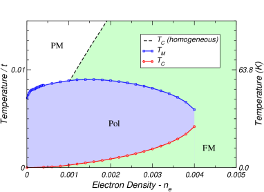
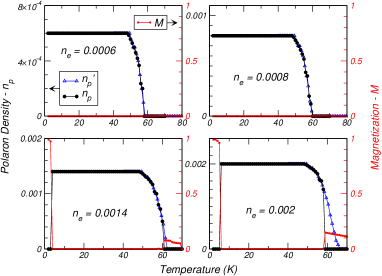
Figure 16: Polaronic stability relative to homogeneous PM/FM phases when a finite band filling is considered. 16 Phase diagram. 16 Each frame shows the equilibrium values of $n_{p}$ and $M$ (order parameters) for total electronic concentrations of $n_{e}=0.0006,\,0.0008,\,0.0014,\,0.0016$. The blue (triangles) curve shows the equilibrium $n_{p}$ that is obtained when only paramagnetism is allowed (i.e. constraining $M=0$).

The overall qualitative features obtained previously in Fig. 4 remain basically the same, the important differences now being: (i) The PM–FM transition curve (dashed line) now places $T_{C}$ for homogeneous phases at higher temperatures than the ones obtained with the de Gennes treatment; (ii) The polaron stability temperature, $T_{m}$, is seen to increase with density if $n_{e}\lesssim 0.001$, just as expected because, the higher the density, the higher the Fermi energy and the more favorable it becomes to create a polaron for the same price in entropy; (iii) The reentrance of the polaronic phase is now very pronounced, being a consequence of (i). It is nonetheless interesting to observe that the critical density for the stabilization of the polaronic phase ($n_{e}\simeq 0.004$) and the typical stabilization temperature, $T_{m}$, are almost exactly the same as the ones encountered in Sec. III.

The nature of the transitions as the temperature is lowered is as follows (see Fig. 16 for reference). Below $n_{e}\simeq 0.001$ the PM–Pol transition is continuous; $n_{p}(T)$ varies continuously from 0 to the saturation value $n_{p}=n_{e}$, and no FM is stabilized except at very low temperatures, below the Pol phase. For $n_{e}\gtrsim 0.001$, FM is stabilized with a continuous PM–FM transition; FM persists only until $T_{m}(n_{e})$ is reached, at which point the polarons set in; the FM–Pol transition is discontinuous because the magnetization drops to zero and $n_{p}$ jumps from 0 to quasi-saturation upon crossing $T_{m}$. This can be seen clearly in the bottom frames of Fig. 16: above $n_{e}\gtrsim 0.001$ the curve $T_{m}$ jumps discontinuously at $T_{m}(n_{e})$ to meet $n_{p}^{\prime}$. At lower temperatures, when the $T_{C}$ line (red/circles) is crossed, the magnetization jumps to the value found in an homogeneous FM phase, concurrently with a discontinuous drop of $n_{p}$ from $n_{e}$ to zero. Notice that the $T_{C}$ line is barely changed by the consideration of a finite band filling. This is related to the fact that, when $T_{C}$ is reached, the polaron density has long since saturated at $n_{e}$, thus emptying the band from carriers.

Appendix B Finite Size Corrections to the Electronic DOS

To estimate the $1/L$ corrections to the ground state energy of an electron gas consider free electrons inside a box of dimensions $L_{x},L_{y}$ and $L_{z}$ Pathria (1996). The electronic spectrum is

$$E_{k}=\frac{\hbar^{2}}{2m}k^{2}\,,\qquad\text{with}\quad\vec{k}=\pi\left(\frac{n_{x}}{L_{x}},\frac{n_{y}}{L_{y}},\frac{n_{z}}{L_{z}}\right)\,,\quad(n_{i}\geq 1)\,.$$ (46)

The integrated DOS will clearly be

$$\Omega(E)=\sum_{n_{x},n_{y},n_{z}\geq 1}\Theta\left(\kappa^{2}-k(n_{x},n_{y},n_{z})^{2}\right)\,,$$ (47)

which corresponds, geometrically, to the set of integers $(n_{x},n_{y},n_{z})$ bounded by the ellipsoid

$$\frac{\kappa^{2}}{\pi^{2}}\geq\frac{n_{x}^{2}}{L_{x}^{2}}+\frac{n_{y}^{2}}{L_{y}^{2}}+\frac{n_{z}^{2}}{L_{z}^{2}}\,.$$ (48)

In the thermodynamic limit, $L_{x,y,z}\to\infty$ and the usual procedure consists in replacing the discrete number of states satisfying (48) by the volume of the ellipsoid in the first octant, divided by the elementary phase space volume. It is obvious that, by doing this, one is either neglecting or overcounting some of the points in phase space that rightfully satisfy (48). This happens mainly at the boundaries, and is all right when $L_{x,y,z}\to\infty$ because the errors are of the order of $1/L$ or $1/L^{2}$ (Fig. 17). However, when $L$ is finite, such corrections are clearly relevant. A particularly important one arises from the fact that, when we calculate the volume of the ellipsoid, the points lying at the coordinate axes are automatically included, whereas from (46) they should not be. So let

$$\Omega^{\prime}(E)=\sum_{n_{x},n_{y},n_{z}}\Theta\left(\kappa^{2}-k(n_{x},n_{y},n_{z})^{2}\right)\,,$$ (49)

with $n_{i}\in\mathbb{Z}$, which relates to $\Omega(E)$ defined in (47) by

$$\Omega^{\prime}(E) =8\,\Omega(E)+\sum_{n_{x},n_{y}}\Theta\left(\kappa^{2}-k(n_{x},n_{y},0)^{2}\right)$$

$$+\sum_{n_{x},n_{z}}\Theta\left(\kappa^{2}-k(n_{x},0,n_{z})^{2}\right)$$

$$+\sum_{n_{y},n_{z}}\Theta\left(\kappa^{2}-k(0,n_{y},n_{z})^{2}\right)$$

$$-\sum_{n_{x}}\Theta\left(\kappa^{2}-k(n_{x},0,0)^{2}\right)$$

$$-\sum_{n_{y}}\Theta\left(\kappa^{2}-k(0,n_{y},0)^{2}\right)$$

$$-\sum_{n_{z}}\Theta\left(\kappa^{2}-k(0,0,n_{z})^{2}\right)+1\,.$$ (50)

The above result reflects the fact that, when calculating the continuum volume enclosed by the ellipsoid, one is adding an extra portion of phase space near the coordinate axes that should not be included, as in Fig. 17. Assuming that $\kappa^{2}/\pi^{2}$ is still reasonably greater than $L_{x}^{-1},L_{z}^{-1}\text{ or }L_{z}^{-1}$, these terms correspond to

$$\Omega^{\prime}(E)\simeq\text{Vol. ellipsoid with axes }L_{x},L_{y},L_{z}\,;$$

$$\sum_{n_{i},n_{j}}\Theta\left(\kappa^{2}-k(n_{i},n_{j},0)^{2}\right)\simeq\text{ Area of ellipse of axes }L_{i},L_{j}\,;$$

$$\sum_{n_{i}}\Theta\left(\kappa^{2}-k(n_{i},0,0)^{2}\right)\simeq\text{ Length of the axis }L_{i}\,.$$ (51)

Therefore, we have that

$$\frac{4}{3}\pi\left(\frac{k}{\pi}\right)^{3}L_{x}L_{y}L_{z}=8\Omega(E)+\pi\left(\frac{k}{\pi}\right)^{2}(L_{x}L_{y}+L_{y}L_{z}+L_{z}L_{x})-2\frac{2}{\pi}(L_{x}+L_{y}+L_{z})+1\,,$$ (52)

implying that the corrected phase space volume is actually

$$\Omega(E)=\frac{\kappa^{3}}{6\pi^{2}}L_{x}L_{y}L_{z}-\frac{\kappa^{2}}{8\pi}(L_{x}L_{y}+L_{y}L_{z}+L_{z}L_{x})+\frac{\kappa}{4\pi}(L_{x}+L_{y}+L_{z})-\frac{1}{8}\,.$$ (53)

There is still the error associated with the under/over estimates of the volume near the surface of the ellipsoid. This gives an additional contribution of the order $\mathcal{O}(\kappa)$ End (i). But since the precise numerical factors are impossible to extract analytically, we do not include this correction. Consequently, the expression above is meaningful only down to $\mathcal{O}(\kappa^{2})$. Given that the volume and surface area of the volume enclosing the electron gas are related to the $L$’s by $L_{x}L_{y}L_{z}=V$ and $L_{x}Ly+L_{y}L_{z}+L_{z}L_{x}=S/2$, the above can be summarized as

$$\Omega(\kappa)\simeq\frac{\kappa^{3}}{6\pi^{2}}V-\frac{\kappa^{2}}{16\pi}S\,,$$ (54)

from which the corrected DOS follows:

$$g(\kappa)=\frac{\partial\Omega(\kappa)}{\partial\kappa}=\frac{k^{2}}{2\pi}V-\frac{k}{8\pi}S=g_{\infty}(\kappa)\left(1-\frac{\pi}{4\kappa}\frac{S}{V}\right)\,.$$ (55)

For instance, taking the leading correction for electrons inside a cubic box ($L_{i}=L$), implies a correction to the ground state energy per electron reading

$$\frac{E}{N_{e}}=\frac{E_{\infty}}{N_{e}}\left[1+\frac{15}{8}\frac{\pi}{L}\left(\frac{1}{6\,\pi^{2}n}\right)^{1/3}\right]\,,$$ (56)

with

$$\frac{E_{\infty}}{N_{e}}=\frac{3}{5}\frac{\hbar^{2}}{2m}\kappa_{F_{\infty}}^{2}\,.$$ (57)

In the main text, we are interested in the corrections to the energy of an electron gas confined to finite sized spherical bubbles. We notice that for a cube of side $L$,

$$\left(\frac{S}{V}\right|_{\text{cube}}=\left(\frac{S}{V}\right|_{\text{inscribed sphere}}\,,$$ (58)

the surface to volume ratio, equals the same ratio for the inscribed sphere with $R=L/2$. Hence we take the result (56) and simply substitute $L$ by $2R$, obtaining

$$\frac{E}{N_{e}}=\frac{E_{\infty}}{N_{e}}\left[1+\frac{15}{16}\left(\frac{\pi}{6\,n}\right)^{1/3}\frac{1}{R}\right]\,,$$ (59)

which provides an estimate of the leading corrections to the ground state (and $T=0$) energy of the confined electron gas.

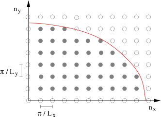
Figure 17: Discrete Phase Space.

References

- de Gennes (1960) P.-G. de Gennes, Phys. Rev. 118, 141 (1960).
- Nagaev (2001) E. L. Nagaev, Phys. Rep. 346, 387 (2001).
- Nagaev (2002) E. L. Nagaev, Colossal Magnetoresistance and Phase Separation in Magnetic Semiconductors (Imperial College Press, 2002).
- Oliver et al. (1972) M. R. Oliver, J. O. Dimmock, A. L. McWhorter, and T. B. Reed, Phys. Rev. B 5, 1078 (1972).
- Torrance et al. (1972) J. B. Torrance, M. W. Shafer, and T. R. McGuire, Phys. Rev. Lett. 29, 1168 (1972).
- Dietl and Spalek (1982) T. Dietl and J. Spalek, Phys. Rev. Lett. 48, 355 (1982).
- Dietl and Spalek (1983) T. Dietl and J. Spalek, Phys. Rev. B 28, 1548 (1983).
- Heiman et al. (1983) D. Heiman, P. A. Wolff, and J. Warnock, Phys. Rev. B 27, 4848 (1983).
- Snow et al. (2001) C. S. Snow, S. L. Cooper, D. P. Young, and Z. Fisk, Phys. Rev. B 64, 174412 (2001).
- Nyhus et al. (1997) P. Nyhus, S. Yoon, M. Kauffman, S. L. Cooper, Z. Fisk, and J. Sarrao, Phys. Rev. B 56, 2717 (1997).
- Teresa et al. (1997) J. M. D. Teresa, M. R. Ibarra, P. A. Algarabel, C. Ritter, C. Marquina, J. Blasco, J. García, A. D. Moral, and Z. Arnold, Nature 386, 256 (1997).
- Amaral et al. (1998) V. S. Amaral, J. P. Araújo, Y. G. Pogorelov, J. B. Sousa, P. B. Tavares, J. M. Vieira, J. M. B. L. dos Santos, A. A. C. S. Lourenço, and P. A. Algarabel, J. Appl. Phys. 83, 7154 (1998).
- Teresa et al. (2000) J. M. D. Teresa, M. R. Ibarra, P. Algarabel, L. Morellon, B. García-Landa, C. Marquina, C. Ritter, A. Maignan, C. Martin, B. Raveau, et al., Phys. Rev. B 65, 100403 (2000).
- Majumdar and Littlewood (1998) P. Majumdar and P. Littlewood, Phys. Rev. Lett. 81, 1314 (1998).
- Kaminski and Sarma (2002) A. Kaminski and S. D. Sarma, Phys. Rev. Lett. 88, 247202 (2002).
- Calderón et al. (2004) M. Calderón, L. Wegener, and P. Littlewood, Phys. Rev. B 70, 92408 (2004).
- Kasuya et al. (1970) T. Kasuya, A. Yanase, and T. Takeda, Solid State Commun. 8, 1543 (1970).
- Mauger (1983) A. Mauger, Phys. Rev. B 27, 2308 (1983).
- Varma (1996) C. M. Varma, Phys. Rev. B 54, 7328 (1996).
- Batista et al. (2000) C. D. Batista, J. Eroles, M. Avignon, and B. Alascio, Phys. Rev. B 62, 15047 (2000).
- Garcia et al. (2002) D. J. Garcia, K. Hallberg, C. D. Batista, S. Capponi, D. Poilblanc, M. Avignon, and B. Alascio, Phys. Rev. B 65, 134444 (2002).
- Meskine et al. (2004) H. Meskine, T. Saha-Dasgupta, and S. Satpathy, Phys. Rev. Lett. 92, 56401 (2004).
- V. M. Pereiraet al. (2004) V. M. Pereira, J. M. B. Lopes dos Santos, E. V. Castro, and A. H. Castro Neto, Phys. Rev. Lett. 93, 147202 (2004).
- Daghofer et al. (2004a) M. Daghofer, W. Koller, H. G. Evertz, and W. von der Linden, cond-mat/0410274 (2004a).
- Daghofer et al. (2004b) M. Daghofer, W. Koller, H. G. Evertz, and W. von der Linden, J. Phys. C: Solid State Physics 16, 5469 (2004b).
- Koller et al. (2003) W. Koller, A. Prüll, H. G. Evertz, and W. von der Linden, Phys. Rev. B 67, 174418 (2003).
- Neuber et al. (2004) D. R. Neuber, M. Daghofer, R. M. Noack, H. G. Evertz, and W. von der Linden, cond-mat/0501251 (2004).
- Pathak and Satpathy (2001) S. Pathak and S. Satpathy, Phys. Rev. B 63, 214413 (2001).
- Wang and J.Freeman (1997) X. Wang and A. J.Freeman, J. Magn. Magn. Mater. 171, 103 (1997).
- Yi et al. (2000) H. Yi, N. H. Hur, and J. Yu, Phys. Rev. B 61, 9501 (2000).
- Nagaev (1998) E. L. Nagaev, Phys. Rev. B 58, 2415 (1998).
- Yunoki et al. (1998) S. Yunoki, J. Hu, A. L. Malavezzi, A. Moreo, N. Furukawa, and E. Dagotto, Phys. Rev. Lett. 80, 845 (1998).
- Arovas et al. (1999) D. P. Arovas, G. Gómez-Santos, and F. Guinea, Phys. Rev. B 59, 13569 (1999).
- Kagan et al. (1999) M. Y. Kagan, D. I. Khomskii, and M. V. Mostovoy, Eur. Phys. J. B 12 (1999).
- Alonso et al. (2001a) J. L. Alonso, L. A. Fernández, F. Guinea, V. Laliena, and V. Martín-Mayor, Phys. Rev. B 63, 54411 (2001a).
- Alonso et al. (2001b) J. L. Alonso, L. A. Fernández, F. Guinea, V. Laliena, and V. Martín-Mayor, Phys. Rev. B 63 (2001b).
- Paschen et al. (2000) S. Paschen, D. Pushin, M. Schlatter, P. Vonlanthen, H. R. Ott, D. P. Young, and Z. Fisk, Phys. Rev. B 61, 4174 (2000).
- Degiorgi et al. (1997) L. Degiorgi, E. Felder, H. R. Ott, J. L. Sarrao, and Z. Fisk, Phys. Rev. Lett. 79, 5134 (1997).
- Pereira (2006) V. M. Pereira, Ph.D. thesis, Universidade do Porto, Porto–Portugal (2006).
- Fisk et al. (1979) Z. Fisk, D. C. Johnston, B. Cornut, S. von Molnar, S. Oseroff, and R. Calvo, J. Appl. Phys. 50, 1911 (1979).
- Guy et al. (1980) C. N. Guy, S. von Molnar, J. Etourneau, and Z. Fisk, Solid State Commun. 33, 1055 (1980).
- Süllow et al. (1998) S. Süllow, I. Prasad, M. C. Aronson, J. L. Sarrao, Z. Fisk, D. H. A. H. Lacerda, M. F. Hundley, A. Vigliante, and D. Gibbs, Phys. Rev. B 57, 5860 (1998).
- Aronson et al. (1999) M. C. Aronson, J. L. Sarrao, Z. Fisk, M. Whitton, and B. L. Brandt, Phys. Rev. B 59, 4720 (1999).
- Rhyee et al. (2003a) J.-S. Rhyee, B. K. Cho, and H.-C. Ri, Phys. Rev. B 67, 125102 (2003a).
- Blomberg et al. (1995) M. K. Blomberg, M. J. Merisalo, M. M. Korsukova, and V. N. Gurin, J. Alloys and Compounds 217, 123 (1995).
- Monnier and Delley (2001) R. Monnier and B. Delley, Phys. Rev. Lett. 87, 157204 (2001).
- Broderick et al. (2003) S. Broderick, L. Degiorgi, H. Ott, J. Sarrao, and Z. Fisk, Eur. Phys. J. B 33, 47 (2003).
- Broderick et al. (2002) S. Broderick, B. Ruzicka, L. Degiorgi, H. R. Ott, J. L. Sarrao, and Z. Fisk, Phys. Rev. B 65, 121102(R) (2002).
- Denlinger et al. (2002) J. D. Denlinger, J. A. Clack, J. W. Allen, G.-H. Gweon, D. M. Poirier, and C. G. Olson, Phys. Rev. Lett. 89, 157601 (2002).
- Giannò et al. (2002) K. Giannò, A. V. Sologubenko, H. R. Ott, A. D. Bianchi, and Z. Fisk, J. Phys.: Condens. Matter 14, 1035 (2002).
- Souma et al. (2003) S. Souma, H. Komatsu, T. Takahashi, R. Kaji, T. Sasaki, Y. Yokoo, and J. Akimitsu, Phys. Rev. Lett. 90, 27202 (2003).
- Rhyee et al. (2003b) J.-S. Rhyee, B. H. Oh, B. K. Cho, M. H. Jung, H. C. Kim, Y. K. Yoon, J. H. Kim, and T. Ekino, cond-mat/0310068 (2003b).
- Doniach (1977) S. Doniach, Physica 91B, 231 (1977).
- Hasegawa and Yanase (1979) A. Hasegawa and A. Yanase, J. Phys. C: Solid State Physics 12, 5431 (1979).
- Dagotto (2003) E. Dagotto, Nanoscale Phase Separation and Colossal Magnetoresistance (Springer Verlag, Berlin, New York, 2003).
- End (a) Interestingly, this result is actually the one we would obtain following the mean-field procedure carried by de Gennes (1960).
- Caimi et al. (2006) G. Caimi, A. Perucchi, L. Degiorgi, H. Ott, V. M. Pereira, A. Castro-Neto, A. Bianchi, and Z. Fisk, Phys. Rev. Lett. 96, 016403 (2006).
- Tsunetsugu et al. (1997) H. Tsunetsugu, M. Sigrist, and K. Ueda, Rev. Mod. Phys. 69, 809 (1997).
- Calderón and Brey (1998) M. J. Calderón and L. Brey, Phys. Rev. B 58, 3286 (1998).
- Haydock et al. (1972) R. Haydock, V. Heine, and M. J. Kelly, J. Phys. C: Solid State Physics 5, 2845 (1972).
- Haydock et al. (1975) R. Haydock, V. Heine, and M. J. Kelly, J. Phys. C: Solid State Physics 8, 2591 (1975).
- End (b) Clearly this is true as far as thermal excitations of the electronic states across the Fermi level are concerned. The electron system will indirectly feel the effects of temperature through the dependence of the DOS on and, consequently, on .
- End (c) Not strictly since in LABEL:~Alonso et al., 2001a the authors used the full fermionic free energy (20), instead of the zero temperature approximation used here. But the differences are barely visible.
- Callen (1985) H. B. Callen, Thermodynamics and an Introduction to Thermostatistics (John Wiley & Sons, 1985).
- End (d) In fact, we can do the Maxwell construction in both the or the diagram. In the latter, the Maxwell construction corresponds to finding the horizontal line that yields exactly Callen (1985).
- End (e) The fact that goes exactly to zero at has to do with the zero temperature approximation used in (22) for the electronic energy. Had we included the Fermi-Dirac distribution in (22) the curve of would go to zero in a seemingly singular way, the result being barely distinguishable for practical purposes from the one plotted in Fig. 9.
- Pines (1963) D. Pines, Elementary Excitations in Solids (Addison-Wesley Publishing Companay, 1963).
- End (f) At first sight it might seem that the electrons are disappearing! In reality it just means that, according to the WS picture, more and more WS cells appear in the system, as diminishes, because the total number of electrons and the total volume are fixed.
- End (g) In order to compare directly with the polaronic stability region, the Langevin entropy was replaced by the Brillouin entropy in the magnetic contribution to the free energy, for consistency. The behavior is the same irrespective of which case is considered, up to global numerical factors.
- Wigner and Seitz (1934) E. Wigner and F. Seitz, pr 46, 509 (1934).
- Jones and Ceperley (1996) M. D. Jones and D. M. Ceperley, Phys. Rev. Lett. 76, 4572 (1996).
- Cândido et al. (2004) L. Cândido, B. Bernu, and D. M. Ceperley, Phys. Rev. B 70, 094413 (2004).
- Ortiz et al. (1999) G. Ortiz, M. Harris, and P. Ballone, Phys. Rev. Lett. 82, 5317 (1999).
- End (h) We are actually allowed to do that since only a few bound states appear beyond the band edge, as can be seen in Fig. 3, and the profile of the bulk DOS is not altered.
- Pathria (1996) R. K. Pathria, Statistical Mechanics (Butterworth-Heinemann, 1996).
- End (i) This can be inspected numerically by plotting the difference between (53) and (47) against . For the difference appears majored by a term linear in .