Geometry of depolarizing channels

Abstract

Depolarizing maps acting on an $N$ dimensional system are completely positive maps resulting into compression of the Bloch ‘ball’ along $N^{2}-1$ polarization directions. In the qubit case these maps are a convex sum of four extremal maps and form a simplex in the space of compression coefficients along the three polarization directions. We calculate the compression domain for three and four level systems. For a three level system the region has curved surfaces, but it is a simplex for a four level system. We conjecture that it is a simplex in the case of $2^{n}$ level systems.

I Introduction

The dynamics of open quantum systems can be described in terms of Completely Positive (CP), trace preserving maps acting on the system 3 ; 4 ; 5 ; 6 ; 7 ; 8 . In general these maps can rotate, compress and translate the Bloch ball, resulting into ‘Affine’ maps 13 . These maps are used to simulate different noises that could be acting on the system 1 ; 2 .

A simple example of noise can be given by depolarizing maps, which result into shrinking of the Bloch ball. In general the compression can be anisotropic, giving a rich geometric structure to the problem. The requirement of complete positivity turns out to be stronger than just positivity. For example, for N=2 the map corresponding to shrinking of the Bloch sphere only along one direction and leaving the other two invariant (pancake map) is not CP. In N=2 case the general depolarizing map has a very simple structure and can be written as a convex sum of four fixed extremal maps. One would like to see if it true for higher dimensional systems.

In what follows we answer the question for N=3 and N=4 cases. We also give a way to answer the question for higher level systems, although we must admit that the calculations becomes much more involved.

Our paper is organized as follows: In Sec. II we briefly describe the geometry of N=2 level depolarizing channels. In Sec. III we show how to calculate the region of positivity for an N dimensional system. We carry out the calculations for N=3 and N=4 cases in Sec. IV and V respectively. We conclude the paper with further discussions in Sec. VI.

II The qubit case

The qubit density matrix is given by

$$\rho=\frac{1}{2}\left(I+a\cdot\sigma\right).$$ (1)

Positivity of $\rho$ requires that $\overrightarrow{a}$ lies inside a sphere with unit radius. Let’s assume that due to depolarization, the sphere shrinks along the three polarization directions by factors of $\nu_{1}$, $\nu_{2}$ and $\nu_{3}$. The natural question arises - what are the allowed values of $\nu_{1}$, $\nu_{2}$ and $\nu_{3}$ to ensure complete positivity of the map?

It turns out 12 that the allowed region in the space of $\nu_{1}$, $\nu_{2}$ and $\nu_{3}$ forms a tetrahedron with vertices at (1,1,1), (1,-1,-1), (-1,1,-1) and (-1,-1,1). These vertices correspond to four extremal maps given by $B_{i}(\rho)=\sigma_{i}\rho\sigma_{i}$, where $i=0,1,2,3$ and $\sigma_{0}=I_{2}$. The general depolarizing map can be written as a convex sum of these maps as

$$B(\rho)=p\sigma_{1}\rho\sigma_{1}+q\sigma_{2}\rho\sigma_{2}+r\sigma_{3}\rho\sigma_{3}+(1-p-q-r)\rho$$ (2)

where p, q, r are non-negative.

Only the region inside the tetrahedron is CP. For example, partial transpose corresponds to the point (1,-1,1) and lies outside the region.

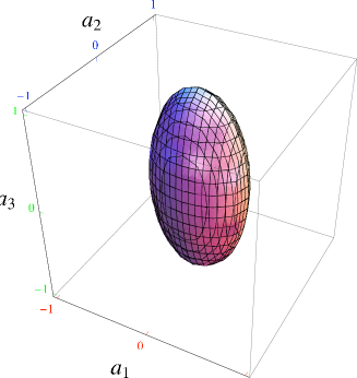
Figure 1: As a result of depolarization the Bloch sphere shrinks anisotropically

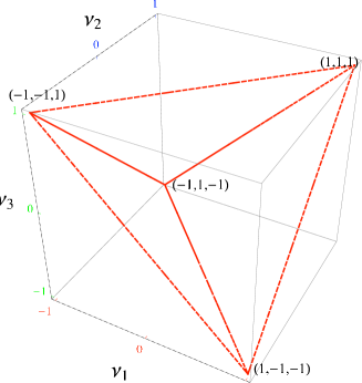
Figure 2: CP region in the space of $\nu$’s is a tetrahedron with vertices corresponding to maps $1\rho 1$, $\sigma_{1}\rho\sigma_{1}$, $\sigma_{2}\rho\sigma_{2}$ and $\sigma_{3}\rho\sigma_{3}$

III The N level system

For an N level system the density matrix can be written in terms of $N^{2}-1$ traceless, Hermitian and trace-orthogonal generators of SU(N), denoted by $J_{i}$, and the polarizations along those directions ($a_{i}$) as

$$\rho=\frac{1}{N}\left(I_{n}+\sqrt{\frac{n(n-1)}{2}}\sum_{i=1}^{N^{2}-1}a_{i}J_{i}\right).$$ (3)

This normalization results into pure states having unit length 10 , analogous to the qubit case.

Let us assume that a general map acting on $\rho$ takes it into another density matrix given by $\rho^{\prime}$. The map can be written in terms of the $A$ matrix3 as:

$$\rho^{\prime}_{rs}=A_{rs,r^{\prime}s^{\prime}}\rho_{r^{\prime}s^{\prime}}.$$ (4)

With change of indices, we can find another matrix B which is Hermitian and has simpler conditions of complete positivity. It is obtained by

$$B_{rr^{\prime},ss^{\prime}}=A_{rs,r^{\prime}s^{\prime}}.$$ (5)

Complete positivity requires B to be positive semi-definite (and thus have non-negative eigenvalues).

III.1 Deriving A from compression of the coherence vector

The simplest way to understand the depolarizing map is to think of it as compression of the coherence vector. Let’s assume that as the result of the map the polarizations are modified as

$$a^{\prime}_{i}=\nu_{i}a_{i}.$$ (6)

which can be considered as a special case of

$$a^{\prime}_{i}=T_{ij}a_{j}=(\delta_{ij}\nu_{j})a_{j}.$$ (7)

For completeness we take T to be $N^{2}\otimes N^{2}$ dimensional matrix acting on the vector (1,$\overrightarrow{a}$). Needless to say, $T_{11}=1$ as required by the trace preserving condition. Both the T and the A matrices contain all the information about the map and are thus related. The relation can be established in the following way.

Since the super-matrix A acts on all the entries in $\rho$, we can convert $\rho$ into a vector (let’s call it $V^{\rho}$) which is acted upon by A. The entries in $V^{\rho}$ are linearly related to the coherence vector as

$$V^{\rho}_{i}=M_{ij}a_{j}$$ (8)

The map takes $V^{\rho}$ to $V^{\rho^{\prime}}$ which is related to $V^{\rho}$ as

$$V^{\rho^{\prime}}=M\cdot a^{\prime}=M\cdot T\cdot a=A\cdot V^{\rho}=A\cdot M\cdot a.$$ (9)

Thus

$$A=M\cdot T\cdot M^{-1}.$$ (10)

Once we get A and B we can find the eigenvalues of B and check for complete positivity. We solve the case of N=3 and N=4 in next two sections.

IV N=3 case

The qutrit density matrix is written as

$$\rho=\frac{1}{3}(1+\sqrt{3}\sum_{i=1}^{8}a_{i}\lambda_{i})$$ (11)

where $\lambda^{\prime}s$ are the Gell-Mann matrices

$$\begin{array}[]{ccc}\lambda_{1}=\left(\begin{array}[]{ccc}0&1&0\\ 1&0&0\\ 0&0&0\end{array}\right),&\lambda_{2}=\left(\begin{array}[]{ccc}0&-i&0\\ i&0&0\\ 0&0&0\end{array}\right),&\lambda_{3}=\left(\begin{array}[]{ccc}1&0&0\\ 0&-1&0\\ 0&0&0\end{array}\right),\\ \lambda_{4}=\left(\begin{array}[]{ccc}0&0&1\\ 0&0&0\\ 1&0&0\end{array}\right),&\lambda_{5}=\left(\begin{array}[]{ccc}0&0&-i\\ 0&0&0\\ i&0&0\end{array}\right),&\lambda_{6}=\left(\begin{array}[]{ccc}0&0&0\\ 0&0&1\\ 0&1&0\end{array}\right),\\ \lambda_{7}=\left(\begin{array}[]{ccc}0&0&0\\ 0&0&-i\\ 0&i&0\end{array}\right),&\lambda_{8}=\frac{1}{\sqrt{3}}\left(\begin{array}[]{ccc}1&0&0\\ 0&1&0\\ 0&0&-2\end{array}\right).&\\ \end{array}$$ (12)

As shown in (7), T can be written as

$$T=diag({1,\nu_{1},\nu_{2},...,\nu_{8}})$$ (13)

M relates the density matrix to the coherence vector as:

$$V^{\rho}_{i}=M_{ij}a_{j}.$$ (14)

Explicitly:

$$\frac{1}{3}\left(\begin{array}[]{c}1+{\sqrt{3}}a_{3}+a_{8}\\ {\sqrt{3}}(a_{1}-ia_{2})\\ {\sqrt{3}}(a_{4}-ia_{5})\\ {\sqrt{3}}(a_{1}+ia_{2})\\ 1-{\sqrt{3}}a_{3}+a_{8}\\ {\sqrt{3}}(a_{6}-ia_{7})\\ {\sqrt{3}}(a_{4}+ia_{5})\\ {\sqrt{3}}(a_{6}+ia_{7})\\ 1-2a_{8}\\ \end{array}\right)=\frac{1}{3}\left(\begin{array}[]{ccccccccc}1&0&0&{\sqrt{3}}&0&0&0&0&1\\ 0&{\sqrt{3}}&-{\sqrt{3}}i&0&0&0&0&0&0\\ 0&0&0&0&{\sqrt{3}}&-{\sqrt{3}}i&0&0&0\\ 0&{\sqrt{3}}&{\sqrt{3}}i&0&0&0&0&0&0\\ 1&0&0&-{\sqrt{3}}&0&0&0&0&1\\ 0&0&0&0&0&0&{\sqrt{3}}&-{\sqrt{3}}i&0\\ 0&0&0&0&{\sqrt{3}}&{\sqrt{3}}i&0&0&0\\ 0&0&0&0&0&0&{\sqrt{3}}&{\sqrt{3}}i&0\\ 1&0&0&0&0&0&0&0&-2\\ \end{array}\right).\left(\begin{array}[]{c}1\\ a_{1}\\ a_{2}\\ a_{3}\\ a_{4}\\ a_{5}\\ a_{6}\\ a_{7}\\ a_{8}\\ \end{array}\right).$$ (15)

Calculation for $A=M\cdot T\cdot M^{-1}$ yields:

$$A=\left(\begin{array}[]{ccccccccc}\frac{1}{3}+\frac{\nu_{3}}{2}+\frac{\nu_{8}}{6}&0&0&0&\frac{1}{3}-\frac{\nu_{3}}{2}+\frac{\nu_{8}}{6}&0&0&0&\frac{1}{3}-\frac{\nu_{8}}{3}\\ 0&\frac{\nu_{1}}{2}+\frac{\nu_{2}}{2}&0&\frac{\nu_{1}}{2}-\frac{\nu_{2}}{2}&0&0&0&0&0\\ 0&0&\frac{\nu_{4}}{2}+\frac{\nu_{5}}{2}&0&0&0&\frac{\nu_{4}}{2}-\frac{\nu_{5}}{2}&0&0\\ 0&\frac{\nu_{1}}{2}-\frac{\nu_{2}}{2}&0&\frac{\nu_{1}}{2}+\frac{\nu_{2}}{2}&0&0&0&0&0\\ \frac{1}{3}-\frac{\nu_{3}}{2}+\frac{\nu_{8}}{6}&0&0&0&\frac{1}{3}+\frac{\nu_{3}}{2}+\frac{\nu_{8}}{6}&0&0&0&\frac{1}{3}-\frac{\nu_{8}}{3}\\ 0&0&0&0&0&\frac{\nu_{6}}{2}+\frac{\nu_{7}}{2}&0&\frac{\nu_{6}}{2}-\frac{\nu_{7}}{2}&0\\ 0&0&\frac{\nu_{4}}{2}-\frac{\nu_{5}}{2}&0&0&0&\frac{\nu_{4}}{2}+\frac{\nu_{5}}{2}&0&0\\ 0&0&0&0&0&\frac{\nu_{6}}{2}-\frac{\nu_{7}}{2}&0&\frac{\nu_{6}}{2}+\frac{\nu_{7}}{2}&0\\ \frac{1}{3}-\frac{\nu_{8}}{3}&0&0&0&\frac{1}{3}-\frac{\nu_{8}}{3}&0&0&0&\frac{1}{3}+\frac{2\nu_{8}}{3}\end{array}\right).$$ (16)

The $B$ matrix is obtained by change of indices as

$$B_{rr^{\prime},ss^{\prime}}=A_{rs,r^{\prime}s^{\prime}}$$ (17)

and is given by:

$$B=\left(\begin{array}[]{ccccccccc}\frac{2+{3\nu_{3}}+{\nu_{8}}}{6}&0&0&0&\frac{{\nu_{1}}}{2}+\frac{{\nu_{2}}}{2}&0&0&0&\frac{{\nu_{4}+\nu_{5}}}{2}\\ 0&\frac{2-3\nu_{3}+{\nu_{8}}}{6}&0&\frac{{\nu_{1}}}{2}-\frac{{\nu_{2}}}{2}&0&0&0&0&0\\ 0&0&\frac{1}{3}-\frac{{\nu_{8}}}{3}&0&0&0&\frac{{\nu_{4}}}{2}-\frac{{\nu_{5}}}{2}&0&0\\ 0&\frac{{\nu_{1}}}{2}-\frac{{\nu_{2}}}{2}&0&\frac{2-3\nu_{3}+{\nu_{8}}}{6}&0&0&0&0&0\\ \frac{{\nu_{1}}}{2}+\frac{{\nu_{2}}}{2}&0&0&0&\frac{2+3\nu_{3}+{\nu_{8}}}{6}&0&0&0&\frac{{\nu_{6}+\nu_{7}}}{2}\\ 0&0&0&0&0&\frac{1}{3}-\frac{{\nu_{8}}}{3}&0&\frac{{\nu_{6}}}{2}-\frac{{\nu_{7}}}{2}&0\\ 0&0&\frac{{\nu_{4}}}{2}-\frac{{\nu_{5}}}{2}&0&0&0&\frac{1}{3}-\frac{{\nu_{8}}}{3}&0&0\\ 0&0&0&0&0&\frac{{\nu_{6}}}{2}-\frac{{\nu_{7}}}{2}&0&\frac{1}{3}-\frac{{\nu_{8}}}{3}&0\\ \frac{{\nu_{4}}}{2}+\frac{{\nu_{5}}}{2}&0&0&0&\frac{{\nu_{6}}}{2}+\frac{{\nu_{7}}}{2}&0&0&0&\frac{1+2\nu_{8}}{3}\\ \end{array}\right).$$ (18)

For the map to be positive, all the eigenvalues should be positive semi-definite. Six of these eigenvalues are given by the ‘hyperplanes’:

$$h_{1}=\lambda_{1} = \frac{1}{6}(2+3\nu_{4}-3\nu_{5}-2\nu_{8})$$

$$h_{2}=\lambda_{2} = \frac{1}{6}(2-3\nu_{4}+3\nu_{5}-2\nu_{8})$$

$$h_{3}=\lambda_{3} = \frac{1}{6}(2+3\nu_{6}-3\nu_{7}-2\nu_{8})$$

$$h_{4}=\lambda_{4} = \frac{1}{6}(2-3\nu_{6}+3\nu_{7}-2\nu_{8})$$

$$h_{5}=\lambda_{5} = \frac{1}{6}(2+3\nu_{1}-3\nu_{2}-3\nu_{3}+\nu_{8})$$

$$h_{6}=\lambda_{6} = \frac{1}{6}(2-3\nu_{1}+3\nu_{2}-3\nu_{3}+\nu_{8})$$

The remaining three eigenvalues are given by the eigenvalues of

$$H=\left(\begin{array}[]{ccc}\frac{2+3\nu_{3}+{\nu_{8}}}{6}&\frac{\nu_{1}+\nu_{2}}{2}&\frac{\nu_{4}+\nu_{5}}{2}\\ \frac{\nu_{1}+\nu_{2}}{2}&\frac{2+3\nu_{3}+{\nu_{8}}}{6}&\frac{\nu_{6}+\nu_{7}}{2}\\ \frac{\nu_{4}+\nu_{5}}{2}&\frac{\nu_{6}+\nu_{7}}{2}&\frac{1+2\nu_{8}}{3}\\ \end{array}\right)$$ (20)

Since the matrix is Hermitian and thus has real roots, the condition of positive eigenvalues translates to $(\lambda_{7}+\lambda_{8}+\lambda_{9}),(\lambda_{7}\lambda_{8}+\lambda_{8}\lambda_{9}+\lambda_{9}\lambda_{7}),\lambda_{7}\lambda_{8}\lambda_{9}$ being positive. These can be easily found from the characteristic equation as

$$h_{7} = \lambda_{7}+\lambda_{8}+\lambda_{9}$$ (21)

$$= 1+\nu_{3}+\nu_{8}$$

$$s_{1} = \lambda_{7}\lambda_{8}+\lambda_{8}\lambda_{9}+\lambda_{9}\lambda_{7}$$ (22)

$$= \frac{1}{12}\left(-3\left(\nu_{1}+\nu_{2}\right){}^{2}+3\nu_{3}^{2}-3\left(\nu_{4}+\nu_{5}\right){}^{2}-3\left(\nu_{6}+\nu_{7}\right){}^{2}+\left(2+\nu_{8}\right)\left(2+3\nu_{8}\right)+2\nu_{3}\left(4+5\nu_{8}\right)\right).$$

$$s_{2} = \lambda_{7}\lambda_{8}\lambda_{9}$$ (23)

$$= \frac{1}{216}(54\nu_{2}(\nu_{4}+\nu_{5})(\nu_{6}+\nu_{7})-18\nu_{1}^{2}(1+2\nu_{8})-18\nu_{2}^{2}(1+2\nu_{8})+18\nu_{1}(3(\nu_{4}+\nu_{5})(\nu_{6}+\nu_{7})-2\nu_{2}(1+2\nu_{8}))$$

$$+ (2+3\nu_{3}+\nu_{8})(4-9(\nu_{4}+\nu_{5}){}^{2}-9(\nu_{6}+\nu_{7}){}^{2}+10\nu_{8}+4\nu_{8}^{2}+6\nu_{3}(1+2\nu_{8}))).$$

Hence we see that the completely positive region is bounded by seven hyperplanes, a second degree surface $s_{1}$ and a third degree surface $s_{2}$. This is quite different from the qubit case where the allowed region is bounded by four planes and is just a simplex with four vertices. For N=3 the depolarizing map has an infinite number of extremal points corresponding to the curved surface.

V N=4 case

From the previous section we might expect that the CP region will be a curved surface for N=4, but quite analogous to the qubit case it turns out to be a simplex.

Let’s start with taking the generators to be: $J$={$I\otimes\sigma_{i}$, $\sigma_{i}\otimes I$, $\sigma_{1}\otimes\sigma_{i}$, $\sigma_{2}\otimes\sigma_{i}$, $\sigma_{3}\otimes\sigma_{i}$} for i=1, 2, 3. The density matrix is written as 9 ; 10 ; 11

$$\rho=\frac{1}{4}(I+\sqrt{6}a\cdot J)$$ (24)

The M matrix is given by:

$$M=\frac{\sqrt{6}}{4}\left(\begin{array}[]{llllllllllllllll}\frac{1}{\sqrt{6}}&0&0&1&0&0&1&0&0&0&0&0&0&0&0&1\\ 0&1&-i&0&0&0&0&0&0&0&0&0&0&1&-i&0\\ 0&0&0&0&1&-i&0&0&0&1&0&0&-i&0&0&0\\ 0&0&0&0&0&0&0&1&-i&0&-i&-1&0&0&0&0\\ 0&1&i&0&0&0&0&0&0&0&0&0&0&1&i&0\\ \frac{1}{\sqrt{6}}&0&0&-1&0&0&1&0&0&0&0&0&0&0&0&-1\\ 0&0&0&0&0&0&0&1&i&0&-i&1&0&0&0&0\\ 0&0&0&0&1&-i&0&0&0&-1&0&0&i&0&0&0\\ 0&0&0&0&1&i&0&0&0&1&0&0&i&0&0&0\\ 0&0&0&0&0&0&0&1&-i&0&i&1&0&0&0&0\\ \frac{1}{\sqrt{6}}&0&0&1&0&0&-1&0&0&0&0&0&0&0&0&-1\\ 0&1&-i&0&0&0&0&0&0&0&0&0&0&-1&i&0\\ 0&0&0&0&0&0&0&1&i&0&i&-1&0&0&0&0\\ 0&0&0&0&1&i&0&0&0&-1&0&0&-i&0&0&0\\ 0&1&i&0&0&0&0&0&0&0&0&0&0&-1&-i&0\\ \frac{1}{\sqrt{6}}&0&0&-1&0&0&-1&0&0&0&0&0&0&0&0&1\end{array}\right)$$ (25)

Let’s take the T matrix as in the previous case

$$T=diag\{1,\nu_{1}...\nu_{15}\}.$$ (26)

B matrix is given by

$$B=\frac{1}{4} \tiny\left(\begin{array}[]{ccccccc}1+\nu_{3}+\nu_{6}+\nu_{15}&0&0&0&0&\nu_{1}+\nu_{2}+\nu_{13}+\nu_{14}&0\\ 0&1-\nu_{3}+\nu_{6}-\nu_{15}&0&0&\nu_{1}-\nu_{2}+\nu_{13}-\nu_{14}&0&0\\ 0&0&1+\nu_{3}-\nu_{6}-\nu_{15}&0&0&0&0\\ 0&0&0&1-\nu_{3}-\nu_{6}+\nu_{15}&0&0&\nu_{1}-\nu_{2}-\nu_{13}+\nu_{14}\\ 0&\nu_{1}-\nu_{2}+\nu_{13}-\nu_{14}&0&0&1-\nu_{3}+\nu_{6}-\nu_{15}&0&0\\ \nu_{1}+\nu_{2}+\nu_{13}+\nu_{14}&0&0&0&0&1+\nu_{3}+\nu_{6}+\nu_{15}&0\\ 0&0&0&\nu_{1}-\nu_{2}-\nu_{13}+\nu_{14}&0&0&1-\nu_{3}-\nu_{6}+\nu_{15}\\ 0&0&\nu_{1}+\nu_{2}-\nu_{13}-\nu_{14}&0&0&0&0\\ 0&0&\nu_{4}-\nu_{5}+\nu_{9}-\nu_{12}&0&0&0&0\\ 0&0&0&\nu_{4}-\nu_{5}-\nu_{9}+\nu_{12}&0&0&\nu_{7}-\nu_{8}-\nu_{10}+\nu_{11}\\ \nu_{4}+\nu_{5}+\nu_{9}+\nu_{12}&0&0&0&0&\nu_{7}+\nu_{8}+\nu_{10}+\nu_{11}&0\\ 0&\nu_{4}+\nu_{5}-\nu_{9}-\nu_{12}&0&0&\nu_{7}-\nu_{8}+\nu_{10}-\nu_{11}&0&0\\ 0&0&0&\nu_{7}-\nu_{8}-\nu_{10}+\nu_{11}&0&0&\nu_{4}-\nu_{5}-\nu_{9}+\nu_{12}\\ 0&0&\nu_{7}+\nu_{8}-\nu_{10}-\nu_{11}&0&0&0&0\\ 0&\nu_{7}-\nu_{8}+\nu_{10}-\nu_{11}&0&0&\nu_{4}+\nu_{5}-\nu_{9}-\nu_{12}&0&0\\ \nu_{7}+\nu_{8}+\nu_{10}+\nu_{11}&0&0&0&0&\nu_{4}+\nu_{5}+\nu_{9}+\nu_{12}&0\end{array}\right|$$ (43)

$$\tiny\left|\begin{array}[]{ccccccc}0&0&0&\nu_{4}+\nu_{5}+\nu_{9}+\nu_{12}&0&0&0\\ 0&0&0&0&\nu_{4}+\nu_{5}-\nu_{9}-\nu_{12}&0&0\\ \nu_{1}+\nu_{2}-\nu_{13}-\nu_{14}&\nu_{4}-\nu_{5}+\nu_{9}-\nu_{12}&0&0&0&0&\nu_{7}+\nu_{8}-\nu_{10}-\nu_{11}\\ 0&0&\nu_{4}-\nu_{5}-\nu_{9}+\nu_{12}&0&0&\nu_{7}-\nu_{8}-\nu_{10}+\nu_{11}&0\\ 0&0&0&0&\nu_{7}-\nu_{8}+\nu_{10}-\nu_{11}&0&0\\ 0&0&0&\nu_{7}+\nu_{8}+\nu_{10}+\nu_{11}&0&0&0\\ 0&0&\nu_{7}-\nu_{8}-\nu_{10}+\nu_{11}&0&0&\nu_{4}-\nu_{5}-\nu_{9}+\nu_{12}&0\\ 1+\nu_{3}-\nu_{6}-\nu_{15}&\nu_{7}+\nu_{8}-\nu_{10}-\nu_{11}&0&0&0&0&\nu_{4}-\nu_{5}+\nu_{9}-\nu_{12}\\ \nu_{7}+\nu_{8}-\nu_{10}-\nu_{11}&1+\nu_{3}-\nu_{6}-\nu_{15}&0&0&0&0&\nu_{1}+\nu_{2}-\nu_{13}-\nu_{14}\\ 0&0&1-\nu_{3}-\nu_{6}+\nu_{15}&0&0&\nu_{1}-\nu_{2}-\nu_{13}+\nu_{14}&0\\ 0&0&0&1+\nu_{3}+\nu_{6}+\nu_{15}&0&0&0\\ 0&0&0&0&1-\nu_{3}+\nu_{6}-\nu_{15}&0&0\\ 0&0&\nu_{1}-\nu_{2}-\nu_{13}+\nu_{14}&0&0&1-\nu_{3}-\nu_{6}+\nu_{15}&0\\ \nu_{4}-\nu_{5}+\nu_{9}-\nu_{12}&\nu_{1}+\nu_{2}-\nu_{13}-\nu_{14}&0&0&0&0&1+\nu_{3}-\nu_{6}-\nu_{15}\\ 0&0&0&0&\nu_{1}-\nu_{2}+\nu_{13}-\nu_{14}&0&0\\ 0&0&0&\nu_{1}+\nu_{2}+\nu_{13}+\nu_{14}&0&0&0\end{array}\right|$$ (60)

$$\tiny\left|\begin{array}[]{cc}0&\nu_{7}+\nu_{8}+\nu_{10}+\nu_{11}\\ \nu_{7}-\nu_{8}+\nu_{10}-\nu_{11}&0\\ 0&0\\ 0&0\\ \nu_{4}+\nu_{5}-\nu_{9}-\nu_{12}&0\\ 0&\nu_{4}+\nu_{5}+\nu_{9}+\nu_{12}\\ 0&0\\ 0&0\\ 0&0\\ 0&0\\ 0&\nu_{1}+\nu_{2}+\nu_{13}+\nu_{14}\\ \nu_{1}-\nu_{2}+\nu_{13}-\nu_{14}&0\\ 0&0\\ 0&0\\ 1-\nu_{3}+\nu_{6}-\nu_{15}&0\\ 0&1+\nu_{3}+\nu_{6}+\nu_{15}\end{array}\right).$$ (77)

The eigenvalues of B are

$$\{\lambda_{i}\}=\{\frac{1}{4}\left(1+\nu_{1}+\nu_{2}+\nu_{3}+\nu_{4}-\nu_{5}-\nu_{6}+\nu_{7}+\nu_{8}+\nu_{9}-\nu_{10}-\nu_{11}-\nu_{12}-\nu_{13}-\nu_{14}-\nu_{15}\right),$$

$$\frac{1}{4}\left(1+\nu_{1}+\nu_{2}+\nu_{3}-\nu_{4}+\nu_{5}-\nu_{6}-\nu_{7}-\nu_{8}-\nu_{9}+\nu_{10}+\nu_{11}+\nu_{12}-\nu_{13}-\nu_{14}-\nu_{15}\right),$$

$$\frac{1}{4}\left(1+\nu_{1}-\nu_{2}-\nu_{3}+\nu_{4}+\nu_{5}+\nu_{6}+\nu_{7}-\nu_{8}-\nu_{9}+\nu_{10}-\nu_{11}-\nu_{12}+\nu_{13}-\nu_{14}-\nu_{15}\right),$$

$$\frac{1}{4}\left(1+\nu_{1}-\nu_{2}-\nu_{3}-\nu_{4}-\nu_{5}+\nu_{6}-\nu_{7}+\nu_{8}+\nu_{9}-\nu_{10}+\nu_{11}+\nu_{12}+\nu_{13}-\nu_{14}-\nu_{15}\right),$$

$$\frac{1}{4}\left(1-\nu_{1}+\nu_{2}-\nu_{3}+\nu_{4}+\nu_{5}+\nu_{6}-\nu_{7}+\nu_{8}-\nu_{9}-\nu_{10}+\nu_{11}-\nu_{12}-\nu_{13}+\nu_{14}-\nu_{15}\right),$$

$$\frac{1}{4}\left(1-\nu_{1}+\nu_{2}-\nu_{3}-\nu_{4}-\nu_{5}+\nu_{6}+\nu_{7}-\nu_{8}+\nu_{9}+\nu_{10}-\nu_{11}+\nu_{12}-\nu_{13}+\nu_{14}-\nu_{15}\right),$$

$$\frac{1}{4}\left(1-\nu_{1}-\nu_{2}+\nu_{3}+\nu_{4}-\nu_{5}-\nu_{6}-\nu_{7}-\nu_{8}+\nu_{9}+\nu_{10}+\nu_{11}-\nu_{12}+\nu_{13}+\nu_{14}-\nu_{15}\right),$$

$$\frac{1}{4}\left(1-\nu_{1}-\nu_{2}+\nu_{3}-\nu_{4}+\nu_{5}-\nu_{6}+\nu_{7}+\nu_{8}-\nu_{9}-\nu_{10}-\nu_{11}+\nu_{12}+\nu_{13}+\nu_{14}-\nu_{15}\right),$$

$$\frac{1}{4}\left(1-\nu_{1}-\nu_{2}+\nu_{3}-\nu_{4}-\nu_{5}+\nu_{6}+\nu_{7}+\nu_{8}-\nu_{9}+\nu_{10}+\nu_{11}-\nu_{12}-\nu_{13}-\nu_{14}+\nu_{15}\right),$$

$$\frac{1}{4}\left(1-\nu_{1}-\nu_{2}+\nu_{3}+\nu_{4}+\nu_{5}+\nu_{6}-\nu_{7}-\nu_{8}+\nu_{9}-\nu_{10}-\nu_{11}+\nu_{12}-\nu_{13}-\nu_{14}+\nu_{15}\right),$$

$$\frac{1}{4}\left(1-\nu_{1}+\nu_{2}-\nu_{3}-\nu_{4}+\nu_{5}-\nu_{6}+\nu_{7}-\nu_{8}+\nu_{9}-\nu_{10}+\nu_{11}-\nu_{12}+\nu_{13}-\nu_{14}+\nu_{15}\right),$$

$$\frac{1}{4}\left(1-\nu_{1}+\nu_{2}-\nu_{3}+\nu_{4}-\nu_{5}-\nu_{6}-\nu_{7}+\nu_{8}-\nu_{9}+\nu_{10}-\nu_{11}+\nu_{12}+\nu_{13}-\nu_{14}+\nu_{15}\right),$$

$$\frac{1}{4}\left(1+\nu_{1}-\nu_{2}-\nu_{3}-\nu_{4}+\nu_{5}-\nu_{6}-\nu_{7}+\nu_{8}+\nu_{9}+\nu_{10}-\nu_{11}-\nu_{12}-\nu_{13}+\nu_{14}+\nu_{15}\right),$$

$$\frac{1}{4}\left(1+\nu_{1}-\nu_{2}-\nu_{3}+\nu_{4}-\nu_{5}-\nu_{6}+\nu_{7}-\nu_{8}-\nu_{9}-\nu_{10}+\nu_{11}+\nu_{12}-\nu_{13}+\nu_{14}+\nu_{15}\right),$$

$$\frac{1}{4}\left(1+\nu_{1}+\nu_{2}+\nu_{3}-\nu_{4}-\nu_{5}+\nu_{6}-\nu_{7}-\nu_{8}-\nu_{9}-\nu_{10}-\nu_{11}-\nu_{12}+\nu_{13}+\nu_{14}+\nu_{15}\right),$$

$$\frac{1}{4}\left(1+\nu_{1}+\nu_{2}+\nu_{3}+\nu_{4}+\nu_{5}+\nu_{6}+\nu_{7}+\nu_{8}+\nu_{9}+\nu_{10}+\nu_{11}+\nu_{12}+\nu_{13}+\nu_{14}+\nu_{15}\right)\}.$$ (78)

Since all of the eigenvalues are hyperplanes, CP region is a simplex. Also, the vertices of this polyhedron correspond to the maps $1\rho 1$, $J_{i}\rho J_{i}$, identical to the qubit maps. The extremal map - $J_{i}\rho J_{i}$ is just a rotation of the Bloch ball about the $J_{i}$ axis. The general depolarizing map can be written as a convex sum of these sixteen extremal maps.

VI Discussion

We found that the general depolarizing map in N=2 and N=4 cases has a simple geometric structure, while for N=3 it is much more complicated. We conjecture that for any $2^{n}$ dimensional case the CP region will be a simplex, with vertices corresponding to a unitary rotation of the Block ball. It would be interesting to explore the extent to which the N=2 and N=4 cases are similar for other maps.

We would also like to point out that our method of calculating B, and thus finding out the region where a map is CP is general and is not restricted to depolarizing maps. The most general map (Affine map) can be easily obtained if we let T also contain translations (see 12 ). In that case T becomes

$$T=\left(\begin{array}[]{cc}1&0\\ \overrightarrow{t}&T^{\prime}\\ \end{array}\right)$$ (79)

where T’ contains only the unital part.

K. D. would like to thank Cesar Rodriguez and Kavan Modi for helpful discussion and suggestions.

References

- (1) M. A. Nielsen and I. L. Chuang. Quantum computation and quantum information. Cambridge university press, Cambridge, U. K., 2000.
- (2) J. Preskill. Quantum computation lecture notes at www.theory.caltech.edu/epreskill/ph219/index.html
- (3) E. C. G. Sudarshan, P. M. Mathews, and J. Rau, Phys. Rev. 121, 920 (1961)
- (4) T. F. Jordan and E. C. G. Sudarshan, J. Math. Phys. 2, 772 (1961).
- (5) T. F. Jordan, M. A. Pinsky, and E. C. G. Sudarshan, J. Math. Phys. 3, 848 (1962).
- (6) E. Størmer, Acta Math. 110, 233 (1963).
- (7) M. D. Choi, Can. J. Math. 24, 520 (1972).
- (8) E. B. Davies, Quantum Theory of Open Systems (Academic Press, New York, 1976).
- (9) L. Jakóbczyk and M. Siennicki, Phys. Lett. A 286, 383(2001).
- (10) M.S. Byrd and N. Khaneja, Phys. Rev. A 68, 062322 (2003).
- (11) Gen Kimura, Phys. Lett. A 314, 339 (2003).
- (12) Mary Beth Ruskai, Stanislaw Szarek, Elisabeth Werner, Lin. Alg. Appl. 347, 159–187 (2002)
- (13) T. F. Jordan, Phys. Rev. A 73, 012106 (2006)