Mechanism of generation of the emission bands
in the dynamic spectrum of the Crab pulsar

Abstract

We show that the proportionately spaced emission bands in the dynamic spectrum of the Crab pulsar (Hankins T. H. & Eilek J. A., 2007, ApJ, 670, 693) fit the oscillations of the square of a Bessel function whose argument exceeds its order. This function has already been encountered in the analysis of the emission from a polarization current with a superluminal distribution pattern: a current whose distribution pattern rotates (with an angular frequency $\omega$) and oscillates (with a frequency $\Omega>\omega$ differing from an integral multiple of $\omega$) at the same time (Ardavan H., Ardavan A. & Singleton J., 2003, J Opt Soc Am A, 20, 2137). Using the results of our earlier analysis, we find that the dependence on frequency of the spacing and width of the observed emission bands can be quantitatively accounted for by an appropriate choice of the value of the single free parameter $\Omega/\omega$. In addition, the value of this parameter, thus implied by Hankins & Eilek’s data, places the last peak in the amplitude of the oscillating Bessel function in question at a frequency ($\sim\Omega^{3}/\omega^{2}$) that agrees with the position of the observed ultraviolet peak in the spectrum of the Crab pulsar. We also show how the suppression of the emission bands by the interference of the contributions from differring polarizations can account for the differences in the time and frequency signatures of the interpulse and the main pulse in the Crab pulsar. Finally, we put the emission bands in the context of the observed continuum spectrum of the Crab pulsar by fitting this broadband spectrum (over 16 orders of magnitude of frequency) with that generated by an electric current with a superluminally rotating distribution pattern.

1 Introduction

Very soon after the discovery of pulsars, it was realized that the very stable periodicity of the mean profiles of their pulses could only result from a source that rotates, and which therefore posesses a rigidly rotating radiation distribution (Gold, 1968). In this paper, we show that this source rotation is not only responsible for the periodicity of the pulses, but also determines the detailed frequency dependence of the emitted radiation. By inferring the values of two adjustable parameters from observational data (values that are consistent with those of plasma frequency and electron cyclotron frequency in a conventional pulsar magnetosphere), and by mildly restricting certain local properties of the source, we are able to account quantitatively for the emission spectrum of the Crab pulsar over 16 orders of magnitude of frequency.

The rigid rotation of the overall distribution pattern of the radiation from a pulsar is described by an electromagnetic field whose distribution depends on the azimuthal angle $\varphi$ only in the combination $(\varphi-\omega t)$, where $\omega$ is the angular frequency of rotation of the pulsar and $t$ is the time. As we show in Appendix A, Maxwell’s equations demand that the charge and current densities that give rise to this radiation field should have the same time dependence. Therefore, the observed motion of the radiation pattern of pulsars can only arise from a source whose distribution pattern rotates rigidly, i.e. a source whose average density depends on $\varphi$ only in the combination $(\varphi-\omega t)$. Furthermore, if a plasma distribution has a rigidly rotating pattern in the emission region, then it must have a rigidly rotating pattern everywhere; we show in Appendix B that a solution of Maxwell’s equations with the time dependence $\partial/\partial t=-\omega\partial/\partial\varphi$ applies either to the entire volume of the magnetospheric plasma distribution or to a region whose boundary is an expanding wave front that will eventually encompass the entire magnetosphere of the pulsar.

Unless the plasma atmosphere surrounding the pulsar is restricted to an unrealistically small volume, it is therefore an inevitable consequence of the observational data that the macroscopic distribution of electric current in the magnetosphere has a rigidly rotating pattern whose linear speed exceeds the speed of light in vacuo $c$ for $r>c/\omega$, where $r$ is the radial distance from the axis of rotation. Although special relativity does not allow a charged particle with a non-zero inertial mass to move faster than $c$, there is no such restriction on the speed of propagation of the variations in a macroscopic charge or current distribution. For instance, the distribution pattern of a polarization current with a propagation speed that exceeds $c$ can be created by the coordinated motion of aggregates of particles that move slower than $c$ (Bolotovskii & Ginzburg, 1972; Ginzburg, 1972; Bolotovskii & Bykov, 1990). Such a polarization-current density is on the same footing as the current density of free charges in the Ampère-Maxwell equation, so that its propagating distribution pattern radiates as would any other moving source of electromagnetic fields (Bolotovskii & Bykov, 1990); indeed, such superluminal polarization currents have been demonstrated to be efficient emitters of radiation in the laboratory (Bessarab et al., 2004; Ardavan et al., 2004b; Singleton et al., 2004; Bolotovskii & Serov, 2005).

Once it is acknowledged that the electric current emitting the observed pulses from pulsars has a superluminally-rotating distribution pattern, results from the published literature on the electrodynamics of superluminal sources (Ardavan, 1998; Ardavan et al., 2003, 2004a, 2007; Schmidt et al., 2007; Ardavan et al., 2008a, b) can be applied to pulsars. In this paper, we explain the recently-observed emission bands in the dynamic spectrum of the Crab pulsar (Hankins & Eilek, 2007) using the calculations of Ardavan et al. (2003). Both the oscillations of the intensity and the frequency dependence of the spacing and width of these bands are described by a Bessel function with a single parameter that is already constrained by other observational data on the spectrum of the Crab pulsar. This Bessel function is characteristic of the spectrum of the radiation by a superluminal polarization current whose distribution pattern rotates (with an angular frequency $\omega$) and oscillates (with a frequency $\Omega>\omega$ differing from an integral multiple of $\omega$) at the same time. It differs from the Bessel function encountered in the analysis of synchrotron radiation only in the relative magnitudes of its argument and its order: while the Bessel function describing synchrotron radiation has an argument smaller than its order and so decays exponentially with increasing frequency, the Bessel function encountered in Ardavan et al. (2003), whose argument exceeds its order, is an oscillatory function of frequency with an amplitude that decays only algebraically. It is this slower decay of the Bessel function in question that endows the emission from a superluminally-rotating source with a broad spectrum. The physical mechanism underlying the broadband nature of this emission is focusing in the time domain (Ardavan et al., 2003, 2008a): contributions toward the intensity of the radiation made over an extended period of emission time are received during a significantly shorter period of observation time.

This paper is organized as follows. Section 2 describes how the most radiatively efficient parts of a pulsar magnetosphere are thin filaments within the superluminally rotating part of its current distribution pattern (Ardavan et al., 2007). A knowledge of the morphology of these filaments (Ardavan et al., 2007), and the ability of a source that travels faster than its own waves to make multiple contributions to the signal received by an observer at a given instant (Ardavan et al., 2004a), are necessary to understand many of the traits of pulsar observations described later in the paper. Section 3 summarizes our earlier analysis (Ardavan et al., 2003) on the frequency spectrum of the radiation from a rotating superluminal source. Using these results, we derive various features of the emission bands in Section 4 and compare them to the frequency bands seen in the interpulses of the Crab pulsar [Figs. 6–8, Hankins & Eilek (2007)]; using a single input parameter, related to the pulsar’s plasma density, we reproduce the observational bands and predict the final ultra-violet emission peak of the Crab pulsar. Section 5 discusses the suppression of the bands by interference; this is relevant to the much less frequency-banded microbursts and nanoshots of the Crab’s main pulses [Figs. 2 and 3, Hankins & Eilek (2007)]. Section 6 describes the continuum spectrum of the Crab pulsar; by introducing a further input parameter related to the plasma dynamics we are able to account quantitatively for the whole emission spectrum over 16 orders of magnitude of frequency. Section 7 gives a short discussion and summary. The mathematical details of our arguments are presented in Appendices A, B and C.

2 The emitting region of a rotating superluminal source: multivalued nature of the retarded time

At large distances from the source, the radiation field of a superluminally rotating extended source at an observation point $P$ is dominated by the emissions of its volume elements that approach $P$ along the radiation direction with the speed of light and zero acceleration at the retarded time (Ardavan et al., 2004a, 2007). These elements constitute a filamentary part of the source whose radial and azimuthal widths become narrower (as $\delta r\sim{R_{P}}^{-2}$ and $\delta\varphi\sim{R_{P}}^{-3}$, respectively), the larger the distance $R_{P}$ of the observer from the source, and whose length is of the order of the length scale $l_{z}$ of the source parallel to the axis of rotation (Ardavan et al., 2007). (Here, $r$, $\varphi$, and $z$ are the cylindrical polar coordinates of the source points.) For an observation point $P$ with spherical polar coordinates ($R_{P},\varphi_{P},\theta_{P}$) that is located in the far zone, this contributing part of the source lies at ${\hat{r}}=\csc\theta_{P},\varphi=\varphi_{P}+3\pi/2$, and is essentially a straight line parallel to the rotation axis, as shown in Fig. 1 (Ardavan et al., 2007). (The dimensionless coordinate ${\hat{r}}$ stands for $r\omega/c$, where $\omega$, the angular frequency of rotation of the distribution pattern of the source, is the same frequency as that with which the pulsar rotates.)

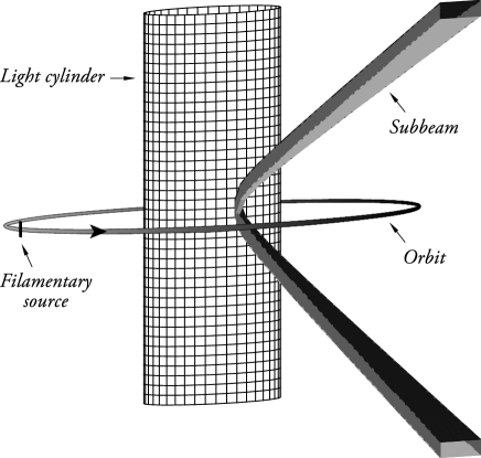
Figure 1: Schematic illustration of the light cylinder $r=c/\omega$, the filamentary part of the distribution pattern of the source that approaches the observation point with the speed of light and zero acceleration at the retarded time, the orbit of this filamentary source, and the subbeam formed by the bundle of cusps that emanate from the constituent volume elements of this filament [after Ardavan et al. (2007)]. The subbeam is diffractionless in the polar direction. The figure represents a snapshot corresponding to a fixed value of the observation time $t_{P}$.

Once a source travels faster than its emitted waves, it can make more than one retarded contribution to the field observed at any given instant (Ardavan et al., 2003, 2004a, 2008a). This multivaluedness of the retarded time means that the wave fronts emitted by each of the contributing elements of the source possess an envelope, which in this case consists of a two-sheeted, tube-like surface whose sheets meet tangentially along a spiraling cusp curve; see Fig. 2 (Ardavan et al., 2004a). For moderate superluminal speeds, the field inside the envelope receives contributions from three distinct values of the retarded time, while the field outside the envelope is influenced only by a single instant of emission time (Schmidt et al., 2007). Coherent superposition of the emitted waves on the envelope (where two of the contributing retarded times coalesce) and on its cusp (where all three of the contributing retarded times coalesce) results in not only a spatial but also a temporal focusing of the waves: the contributions from emission over an extended period of retarded time reach an observer who is located on the cusp during a significantly shorter period of observation time (Ardavan et al., 2008a).

The field of each contributing volume element of the source is strongest, therefore, on the cusp of the envelope of wave fronts that it emits [see Ardavan et al. (2007) and references therein]. The bundle of cusps generated by the collection of the contributing source elements (i.e. by the filamentary part of the source that approaches the observer with the speed of light and zero acceleration) constitutes a radiation subbeam whose widths in the polar and azimuthal directions are of the order of $\delta\theta_{P}\sim{R_{P}}^{-1}$ and $\delta\varphi_{P}\sim{R_{P}}^{-3}$, respectively (Ardavan et al., 2007). The overall radiation beam generated by the source consists of a (necessarily incoherent) superposition of such subbeams. This beam’s azimuthal width is the same as the azimuthal extent of the source, and its polar width, $\arccos(1/{\hat{r}}_{<})\leq|\theta_{P}-\pi/2|\leq\arccos(1/{\hat{r}}_{>})$, is determined by the radial extent $1<{\hat{r}}_{<}\leq{\hat{r}}\leq{\hat{r}}_{>}$ of the superluminal part of the source (Ardavan et al., 2007). This will be important in Secs. 4 and 5; the $\varphi_{P}$ dependence of the radiation intensity within the overall beam (i.e. what is observed as the main pulse, interpulse, and other components of the mean pulse) thus reflects the distribution of the source density around the cylindrical surface ${\hat{r}}=\csc\theta_{P}$ from which the main contributions to the field arise.

Since the cusps represent the loci of points at which the emitted spherical waves interfere constructively [i.e. represent wave packets that are constantly dispersed and reconstructed out of other waves (Ardavan, 1998)], the subbeams generated by a superluminal source need not be subject to diffraction as are conventional radiation beams. Nevertheless, they have a decreasing angular width (i.e. are nondiffracting) only in the polar direction (Ardavan et al., 2007). Their azimuthal width $\delta\varphi_{P}$ decreases as ${R_{P}}^{-3}$ with distance because they receive contributions from an azimuthal extent $\delta\varphi$ of the source that likewise shrinks as ${R_{P}}^{-3}$. They would have had a constant azimuthal width had the azimuthal extent of the contributing part of the source been independent of $R_{P}$. On the other hand, the solid angle occupied by the cusps has a thickness $\delta z_{P}$ in the direction parallel to the rotation axis that remains of the order of the height $l_{z}$ of the source distribution at all distances (see Fig. 1). Consequently, the polar width $\delta\theta_{P}$ of the particular subbeam that goes through the observation point decreases as ${R_{P}}^{-1}$, instead of being independent of $R_{P}$ (Ardavan et al., 2007).

Because it has a constant linear width parallel to the rotation axis, an individual subbeam subtends an area of the order of $R_{P}$, rather than ${R_{P}}^{2}$. In order that the energy flux remain the same across all cross sections of the subbeam, therefore, it is essential that the Poynting vector associated with this radiation correspondingly decay more slowly than that of a conventional, spherically decaying beam: as ${R_{P}}^{-1}$, rather than ${R_{P}}^{-2}$, within the bundle of cusps that emanate from the constituent volume elements of the source and extend into the far zone (Ardavan et al., 2004a). This result, which also follows from the superposition of the Liénard-Wiechert fields of the constituent volume elements of a rotating superluminal source (Ardavan et al., 2007), has been demonstrated experimentally (Ardavan et al., 2004b; Singleton et al., 2004).

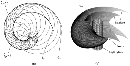
Figure 2: (a) Cross section of the Čerenkov-like envelope (bold curves) of the spherical Huygens wave fronts (fine circles) emitted by a volume element $S$ within the distribution pattern of an extended, rotating superluminal source of angular frequency $\omega$ [after Ardavan et al. (2004a)]. The point $S$ is on a circle of radius $r=2.5\,c/\omega$, or ${\hat{r}}\equiv r\omega/c=2.5$, i.e. has an instantaneous linear velocity $r\omega=2.5\,c$. The cross section is with the plane of $S$’s orbit; dashed circles designate the light cylinder $r_{P}=c/\omega$ (${\hat{r}}_{P}=1$) and the orbit of $S$. (b) Three-dimensional view of the light cylinder, the envelope of wave fronts emanating from $S$, and the cusp along which the two sheets of this envelope meet tangentially. The cusp is tangent to the light cylinder in the plane of the orbit and spirals outward into the far zone.

The fact that the observationally-inferred dimensions of the plasma structures responsible for the emission from pulsars are less than $1$ metre in size (Hankins et al., 2003) reflects, in the present context, the narrowing (as ${R_{P}}^{-2}$ and ${R_{P}}^{-3}$, respectively) of the radial and azimuthal dimensions of the filamentary part of the source that approaches the observer with the speed of light and zero acceleration at the retarded time. Not only do the nondiffracting subbeams that emanate from such filaments account for the nanostructure, and so the brightness temperature, of the giant pulses, but the nonspherical decay of the intensity of such subbeams (as ${R_{P}}^{-1}$ instead of ${R_{P}}^{-2}$) explains why their energy densities at their source appear to exceed the energy densities of both the plasma and the magnetic field at the suface of a neutron star when estimated on the basis of the inverse square law (Soglanov et al., 2004).

3 Frequency spectrum of the radiation from a rotating superluminal source

In this section we summarize the results of Ardavan et al. (2003) relevant to pulsars; the original intent of that paper was to calculate the spectrum of the radiation from a generic superluminal source that has been implemented in the laboratory (Ardavan et al., 2004b; Singleton et al., 2004). This source comprises a polarization-current density ${\bf j}=\partial{\bf P}/\partial t$ for which

$$P_{r,\varphi,z}(r,\varphi,z,t) = s_{r,\varphi,z}(r,z)\cos(m\hat{\varphi})\cos(\Omega t),$$ (1)

$$\qquad\qquad\qquad\qquad-\pi<\hat{\varphi}\leq\pi,$$

with

$$\hat{\varphi}\equiv\varphi-\omega t,$$ (2)

where $P_{r,\varphi,z}$ are the components of the polarization ${\bf{\it P}}$ in a cylindrical coordinate system ($r,\varphi,z$) based on the axis of rotation, ${\bf s}(r,z)$ is an arbitrary vector that vanishes outside a finite region of the $(r,z)$ space, and $m$ is a positive integer. For a fixed value of $t$, the azimuthal dependence of the polarization (1) along each circle of radius $r$ within the source is the same as that of a sinusoidal wave train with the wavelength $2\pi r/m$ whose $m$ cycles fit around the circumference of the circle smoothly. As time elapses, this wave train both propagates around each circle with the velocity $r\omega$ and oscillates in its amplitude with the frequency $\Omega$. This is a generic source: one can construct any distribution with a uniformly rotating pattern, $P_{r,\varphi,z}(r,\hat{\varphi},z)$ or $j_{r,\varphi,z}(r,\hat{\varphi},z)$, by the superposition over $m$ of terms of the form $s_{r,\varphi,z}(r,z,m)\cos(m\hat{\varphi})$. In the following discussion, we assume that the modulation frequency $\Omega$ is positive and different from an exact integral multiple of the rotation frequency $\omega$ [for the significance of this incommensurablity requirement, see Ardavan et al. (2003)].

Although formulated in terms of a polarization current (for which there is manifestly no restriction on the propagation speed of the variations in the current density), the results that follow hold true for any current distribution whose density depends on $\varphi$ as $\varphi-\omega t$ in $r>c/\omega$. The electromagnetic fields

$${\bf E}=-{\bf\nabla}_{P}A^{0}-c^{-1}\partial{\bf A}/\partial t_{P},\quad{\bf B}={\bf\nabla}_{P}{\bf\times A},$$ (3)

that arise from such a source are given, in the absence of boundaries, by the following classical expression for the retarded four-potential:

$$A^{\mu}({\bf x}_{P},t_{P}) = c^{-1}\int{\rm d}^{3}x{\rm d}t\,j^{\mu}({\bf x},t)\delta(t_{P}-t-R/c)/R$$ (4)

$$\qquad\qquad\qquad\qquad\qquad\mu=0,\cdots,3.$$

Here, $({\bf x}_{P},t_{P})=(r_{P},\varphi_{P},z_{P},t_{P})$ and $({\bf x},t)=(r,\varphi,z,t)$ are the space-time coordinates of the observation point and the source points, respectively, $R$ stands for the magnitude of ${\bf R}\equiv{\bf x}_{P}-{\bf x}$, and $\mu=1,2,3$ designate the spatial components, ${\bf A}$ and ${\bf j}$, of $A^{\mu}$ and $j^{\mu}$ in a Cartesian coordinate system (Jackson, 1999).

In Ardavan et al. (2003), we first calculated the Liénard-Wiechert field that arises from a circularly moving point source (representing a volume element of an extended source) with a superluminal speed $r\omega>c$, i.e. considered a generalization of the synchrotron radiation to the superluminal regime. We then evaluated the integral representing the retarded field of the extended source (1) by superposing the fields generated by the constituent volume elements of this source, i.e. by using the generalization of the synchrotron field as the Green’s function for the problem [see equation (19) of Ardavan et al. (2003)]. For a source that travels faster than $c$, this Green’s function has extended singularities arising from the constructive interference of the emitted waves on the envelope of wave fronts and its cusp (see Fig. 2).

Correspondingly, the fields ${\bf E}$ and ${\bf B}$ are given, in the frequency domain, by radiation integrals with rapidly oscillating integrands whose phases are stationary on the loci of the coherently contributing source elements: those source elements that approach the observer, along the radiation direction, with the speed of light and zero acceleration at the retarded time. For a radiation angular frequency $n\omega$ that appreciably exceeds the angular velocity $\omega$, these integrals can be evaluated by the method of stationary phase to obtain the following expression for the electric field of the emitted radiation outside the plane of the source’s orbit:

$${\bf E}=\Re\left\{{\tilde{\bf E}}_{0}+2\sum_{n=1}^{\infty}{\tilde{\bf E}}_{n}\exp(-{\rm i}n{\hat{\varphi}}_{P})\right\},$$ (5)

in which

$${\tilde{\bf E}}_{n} \simeq {\textstyle\frac{1}{2}}{{\hat{r}}_{P}}^{-1}\exp\{-{\rm i}[n({\hat{R}}_{P}+{\textstyle\frac{3}{2}}\pi)-(\Omega/\omega)(\varphi_{P}+{\textstyle\frac{3}{2}}\pi)]\}$$ (6)

$$\times Q_{\hat{\varphi}}{\bar{Q}}_{r}{\bar{\bf Q}}_{z}+\{m\to-m,\Omega\to-\Omega\},$$

$$Q_{\hat{\varphi}}=(-1)^{n+m}\sin\left(\frac{\pi\Omega}{\omega}\right)\left(\frac{{\mu_{+}}^{2}}{n-\mu_{+}}+\frac{{\mu_{-}}^{2}}{n-\mu_{-}}\right),$$ (7)

$${\bar{Q}}_{r}\simeq{\hat{r}}_{>}-{\hat{r}}_{<},\qquad n\ll\pi{\hat{R}}_{P}/({\hat{r}}_{>}-{\hat{r}}_{<})^{2},$$ (8)

or

$${\bar{Q}}_{r}\simeq(2\pi{\hat{R}}_{P}/n)^{1/2}\exp(-{\rm i}\pi/4),\qquad n\gg\pi{\hat{R}}_{P}/({\hat{r}}_{>}-{\hat{r}}_{<})^{2},$$ (9)

and

$${\bar{\bf Q}}_{z} = \big{[}{\bar{s}}_{r}{\bf J}_{n-\Omega/\omega}(n)+{\rm i}{\bar{s}}_{\varphi}{{\bf J}^{\prime}}_{n-\Omega/\omega}(n)\big{]}{\hat{\bf e}}_{\parallel}$$ (10)

$$+\big{[}({\bar{s}}_{\varphi}\cos\theta_{P}-{\bar{s}}_{z}\sin\theta_{P}){\bf J}_{n-\Omega/\omega}(n)$$

$$\qquad-{\rm i}{\bar{s}}_{r}\cos\theta_{P}{{\bf J}^{\prime}}_{n-\Omega/\omega}(n)\big{]}{\hat{\bf e}}_{\perp},$$

with

$${\bar{s}}_{r,\varphi,z}\equiv\int_{-\infty}^{\infty}{\rm d}{\hat{z}}\,\exp({\rm i}n{\hat{z}}\cos\theta_{P})s_{r,\varphi,z}\big{|}_{{\hat{r}}=\csc\theta_{P}}$$ (11)

[see equations (15), (23), (46) and (66)–(68) of Ardavan et al. (2003)]. Here, $({\hat{r}},{\hat{z}};{\hat{r}}_{P},{\hat{z}}_{P})$ stand for $(r\omega/c,z\omega/c;r_{P}\omega/c,z_{P}\omega/c)$, $(R_{P},\theta_{P},\varphi_{P})$ are the spherical polar coordintes of the observation point $P$, $\mu_{\pm}\equiv(\Omega/\omega)\pm m$, ${\hat{r}}_{<}<1$ and ${\hat{r}}_{>}>1$ are the upper and lower limits of the radial interval in which the source densities $s_{r,\varphi,z}$ are non-zero, ${\bf J}$ and ${\bf J}^{\prime}$ are the Anger function and the derivative of the Anger function with respect to its argument, respectively, and ${\hat{\bf e}}_{\parallel}\equiv{\hat{\bf e}}_{z}\times{\hat{\bf n}}/|{\hat{\bf e}}_{z}\times{\hat{\bf n}}|$ (which is parallel to the plane of rotation) and ${\hat{\bf e}}_{\perp}\equiv{\hat{\bf n}}{\bf\times}{\hat{\bf e}}_{\parallel}$ comprise a pair of unit vectors normal to the radiation direction ${\hat{\bf n}}$ (${\hat{\bf e}}_{z}$ is the base vector associated with the coordinate $z$). The symbol $\{m\to-m,\Omega\to-\Omega\}$ designates a term exactly like the one preceding it but in which $m$ and $\Omega$ are everywhere replaced by $-m$ and $-\Omega$, respectively.

The radiated power per harmonic per unit solid angle is therefore given by

$${\rm d}P_{n}/{\rm d}\Omega_{P} = (2\pi)^{-1}c{R_{P}}^{2}|{\tilde{\bf E}}_{n}|^{2}$$ (12)

$$\simeq (8\pi)^{-1}(c^{3}/\omega^{2})\csc^{2}\theta_{P}|{\bar{Q}}_{r}|^{2}{Q_{\hat{\varphi}}}^{2}|{\bar{\bf Q}}_{z}|^{2},$$

where ${\rm d}\Omega_{P}$ denotes the element $\sin\theta_{P}{\rm d}\theta_{P}{\rm d}\varphi_{P}$ of solid angle in the space of observation points. The contribution of the term $\{m\to-m,\Omega\to-\Omega\}$ in equation (6) has been ignored here because the Anger functions for $-\Omega<0$ turn out to be exponentially smaller than those for positive $\Omega$ (see Appendix C).

There is no difference between an Anger function, ${\bf J}_{\nu}(\chi)$, and a Bessel function of the first kind, $J_{\nu}(\chi)$, when $\nu$ is an integer. Even for a non-integral value of $\nu$, the difference between these two functions vanishes, as $\chi^{-1}$, if $\chi\gg 1$. In the regime $n\gg 1$, where the radiation frequency $n\omega$ appreciably exceeds the rotation frequency, therefore, the Anger functions ${\bf J}_{n-\Omega/\omega}(n)$ and ${{\bf J}^{\prime}}_{n-\Omega/\omega}(n)$ in Equation (10) can be replaced by the Bessel functions $J_{n-\Omega/\omega}(n)$ and ${J^{\prime}}_{n-\Omega/\omega}(n)$, respectively. If the radiation frequency $n\omega$ appreciably exceeds also the modulation frequency $\Omega$, then these Bessel functions can in turn be approximated by the following Airy functions:

$$J_{n-\frac{\Omega}{\omega}}(n)\simeq\left(\frac{2}{n}\right)^{1/3}{\rm Ai}\left[-\left(\frac{2}{n}\right)^{1/3}\frac{\Omega}{\omega}\right],$$ (13)

$${J^{\prime}}_{n-\frac{\Omega}{\omega}}(n)\simeq-\left(\frac{2}{n}\right)^{2/3}{\rm Ai}^{\prime}\left[-\left(\frac{2}{n}\right)^{1/3}\frac{\Omega}{\omega}\right],$$ (14)

where ${\rm Ai}^{\prime}$ stands for the derivative of the Airy function with respect to its argument (see Appendix C).

Hence, the radiated power is given by

$$\frac{{\rm d}P_{n}}{{\rm d}\Omega_{P}} \simeq \frac{c^{3}}{8\pi^{2}\omega^{2}}\csc^{2}\theta_{P}|{\bar{Q}}_{r}|^{2}{Q_{\hat{\varphi}}}^{2}$$ (15)

$$\times\left(\frac{2}{n}\right)^{2/3}\Bigg{|}\left[{\bar{s}}_{r}{\hat{\bf e}}_{\parallel}+({\bar{s}}_{\varphi}\cos\theta_{P}-{\bar{s}}_{z}\sin\theta_{P}){\hat{\bf e}}_{\perp}\right]$$

$$\times{\rm Ai}\left[-\left(\frac{2}{n}\right)^{1/3}\frac{\Omega}{\omega}\right]-{\rm i}({\bar{s}}_{\varphi}{\hat{\bf e}}_{\parallel}+{\bar{s}}_{r}\cos\theta_{P}{\hat{\bf e}}_{\perp})$$

$$\times\left(\frac{2}{n}\right)^{1/3}{\rm Ai}^{\prime}\left[-\left(\frac{2}{n}\right)^{1/3}\frac{\Omega}{\omega}\right]\Bigg{|}^{2}$$

in the regime where the radiation frequency ($n\omega$) apprecialy exceeds both the rotation ($\omega$) and modulation ($\Omega$) frequencies of the source distribution (1).

Asymptotic values of the amplitudes of ${\rm Ai}[-(2/n)^{1/3}(\Omega/\omega)]$ and ${\rm Ai}^{\prime}[-(2/n)^{1/3}(\Omega/\omega)]$ are respectively given by $(2/n)^{-1/12}(\Omega/\omega)^{-1/4}$ and $(2/n)^{1/12}(\Omega/\omega)^{1/4}$, when $n\ll(\Omega/\omega)^{3}$, and by the constants ${\rm Ai}(0)$ and ${\rm Ai}^{\prime}(0)$ when $n\gg(\Omega/\omega)^{3}$ (Abramowitz & Stegun, 1970). Moreover, the quantity $Q_{\hat{\varphi}}$, which appears in equation (15), is independent of $n$ ($\sim 2\Omega/\omega$) if $n\ll\mu_{+}$, decays as $n^{-1}$ if $n\gg\mu_{+}$, and is of the order of $n$ if $n\simeq m\gg\Omega/\omega$ [see equation(7)].

Depending on the relative magnitudes of $n$, $m$ and $\Omega/\omega$, therefore, the amplitude of the radiated power ${\rm d}P_{n}/{\rm d}\Omega_{P}$ decays with the harmonic number $n$ as $n^{-\sigma}|{\bar{s}}_{r,\varphi,z}(n)|^{2}$, where the exponent $\sigma$ can assume one of the values $1/2$, $2/3$, $5/2$ or $8/3$, and ${\bar{s}}_{r,\varphi,z}(n)$ denotes the frequency dependence of the Fourier components of the source densities $s_{r,\varphi,z}$. The way in which ${\bar{s}}_{r,\varphi,z}(n)$ decay with $n$, for large $n$, is determined by the distribution of the source density ${\bf s}(r,z)$ with respect to $z$ [see equation (11)], and so is model-dependent. However, the spacings between the emission bands predicted by equation (15) turn out to be essentially independent of the rate of decay of the amplitudes of these bands (see below).

Having assembled the relevant equations, we now compare their predictions with established observational data on the Crab pulsar.

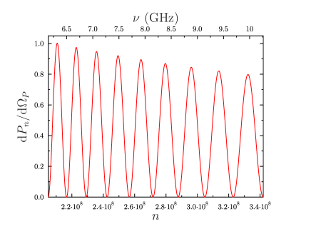
Figure 3: The power ${\rm d}P_{n}/{\rm d}\Omega_{P}$ radiated per harmonic per unit solid angle (in arbitrary units), into the signal linearly polarized parallel to the plane of rotation, versus the harmonic number $n$ (lower axis) for $\Omega/\omega=1.9\times 10^{4}$, $a_{\parallel}=1.48\times 10^{-5}$ and $b_{\parallel}=1.03\times 10^{4}$. The upper axis gives observation frequency $n\omega/2\pi$ for the case of the Crab pulsar [$\omega/(2\pi)\simeq 30$ Hz]. The spacing, the width, and the number of oscillations in this figure are the same as those of the bands seen in the interpulse data from the Crab pulsar over the frequency interval $8<\nu<10.5$ GHz [see Figs. 6–8; Hankins & Eilek (2007)].

4 Predicted frequency bands: comparison with the spectra of the Crab interpulses

One of the most remarkable features of the observational data from the Crab pulsar is the presence of well-defined frequency bands within the midpulses (Hankins & Eilek, 2007). We now show that these are a natural consequence of a rotating superluminal source and use their spacing to predict the high-frequency emission of the Crab pulsar.

When the absolute value of their argument appreciably exceeds unity, the Airy functions in equation (15) are rapidly oscillating functions of the harmonic number $n$ with peaks that spread further apart with increasing $n$ (Fig. 3). The rate of increase of the spacing between the peaks in question is determined solely by the value of $\Omega/\omega$. We now derive an explicit expression for the spacing $\Delta n$ of the maxima of the radiated power ${\rm d}P_{n}/{\rm d}\Omega_{P}$ as a function of $n$ and compare the result with the proportionately spaced emission bands observed by Hankins & Eilek (2007).

Within the range $\Omega/\omega\ll n\ll(\Omega/\omega)^{3}$ of harmonic numbers, where they are oscillatory, the Airy functions in equation (15) can be further approximated by

$${\rm Ai}[-(2/n)^{1/3}(\Omega/\omega)]\simeq\pi^{-1/2}(n/2)^{1/12}(\Omega/\omega)^{-1/4}\cos\psi$$ (16)

and

$${\rm Ai}^{\prime}[-(2/n)^{1/3}(\Omega/\omega)]\simeq\pi^{-1/2}(n/2)^{-1/12}(\Omega/\omega)^{1/4}\sin\psi$$ (17)

where

$$\psi\equiv\textstyle{2\over 3}(2/n)^{1/2}(\Omega/\omega)^{3/2}-\pi/4$$ (18)

(see Appendix C). In this regime, therefore, equation (15) reduces to

$$\frac{{\rm d}P_{n}}{{\rm d}\Omega_{P}}\simeq\frac{c^{3}\csc^{2}\theta_{P}}{8\pi^{2}\omega^{2}}|{\bar{Q}}_{r}|^{2}{Q_{\hat{\varphi}}}^{2}\left(\frac{2\omega}{n\Omega}\right)^{1/2}\big{|}{\cal P}_{\parallel}{\hat{\bf e}}_{\parallel}+{\cal P}_{\perp}{\hat{\bf e}}_{\perp}\big{|}^{2},$$ (19)

in which

$${\cal P}_{\parallel}\equiv{\bar{s}}_{r}\cos\psi-{\rm i}\left(\frac{2\Omega}{n\omega}\right)^{1/2}{\bar{s}}_{\varphi}\sin\psi$$ (20)

and

$${\cal P}_{\perp}\equiv({\bar{s}}_{\varphi}\cos\theta_{P}-{\bar{s}}_{z}\sin\theta_{P})\cos\psi-{\rm i}\frac{2\Omega}{n\omega}{\bar{s}}_{r}\cos\theta_{P}\sin\psi$$ (21)

represent the contributions towards the radiated field ${\tilde{\bf E}}_{n}$ from differing polarizations.

Let us first consider the contribution towards the radiated power from the component of the field parallel to the plane of rotation. It follows from equation (20) that

$$|{\cal P}_{\parallel}|^{2} = \sec(2\gamma_{\parallel})\big{\{}-|{\bar{s}}_{r}|^{2}\sin^{2}\gamma_{\parallel}+\frac{2\Omega}{n\omega}|{\bar{s}}_{\varphi}|^{2}\cos^{2}\gamma_{\parallel}$$ (22)

$$+[|{\bar{s}}_{r}|^{2}-\frac{2\Omega}{n\omega}|{\bar{s}}_{\varphi}|^{2}]\cos^{2}(\psi-\gamma_{\parallel})\big{\}},$$

where

$$\gamma_{\parallel}=\textstyle{1\over 2}\arctan\frac{[2\Omega/(n\omega)]^{1/2}\Im\{{\bar{s}}_{r}{{\bar{s}}_{\varphi}}^{*}\}}{|{\bar{s}}_{r}|^{2}-[2\Omega/(n\omega)]|{\bar{s}}_{\varphi}|^{2}},$$ (23)

with $\Im$ and $*$ denoting the imaginary part and a complex conjugate, respectively. Two successive oscillations of $|{\cal P}_{\parallel}|^{2}$ in the neighbourhood of any given $n$ arise, according to equation (22), from a change in the value of the argument of $\cos^{2}(\psi-\gamma_{\parallel})$ by $\pi$. Therefore, the spacing between two successive peaks of this function is locally given by

$$\Delta n=\pi\big{|}\frac{\partial}{\partial n}(\psi-\gamma_{\parallel})\big{|}^{-1},$$ (24)

an equation that yields $\Delta n$ versus $n$ for all $n$.

If the source densities ${\bar{s}}_{r,\varphi,z}$ have a weak dependence on $n$, then the high-frequency ($n\gg 1$) limits of equations (22) and (23) assume the simple forms

$$|{\cal P}_{\parallel}|^{2}\simeq|{\bar{s}}_{r}|^{2}\cos^{2}(\psi-\gamma_{\parallel}),$$ (25)

and

$$\gamma_{\parallel} \simeq \left(\frac{2\Omega}{n\omega}\right)^{1/2}\frac{\Im\{{\bar{s}}_{r}{{\bar{s}}_{\varphi}}^{*}\}}{|{\bar{s}}_{r}|^{2}}$$ (26)

$$\simeq [2\Omega/(n\omega)]^{1/2}[a_{\parallel}+b_{\parallel}(n-n_{0})],$$

where

$$a_{\parallel}\equiv\frac{\Im\{{\bar{s}}_{r}{{\bar{s}}_{\varphi}}^{*}\}}{|{\bar{s}}_{r}|^{2}}\Bigg{|}_{n=n_{0}},$$ (27)

and

$$b_{\parallel}\equiv\frac{\partial}{\partial n}\left[\frac{\Im\{{\bar{s}}_{r}{{\bar{s}}_{\varphi}}^{*}\}}{|{\bar{s}}_{r}|^{2}}\right]\Bigg{|}_{n=n_{0}}.$$ (28)

denote the first two coefficients in the Taylor expansion of $\Im\{{\bar{s}}_{r}{{\bar{s}}_{\varphi}}^{*}\}/|{\bar{s}}_{r}|^{2}$ about a local value $n_{0}$ of $n$.

In this case, equation (24), together with equations (18) and (25)–(28), yields explicit expressions both for the radiated power $|{\cal P}_{\parallel}|^{2}$ and for the spacing $\Delta n$ between its successive peaks. These expressions are plotted in Figs. 3 and 4 over the interval $2\times 10^{8}\leq n\leq 3.5\times 10^{8}$. In the case of the Crab pulsar, where the rotational frequency $\omega/(2\pi)$ is approximately $30$ Hz, the interval of harmonic numbers shown in Figs. 3 and 4 corresponds to a frequency [$\nu=n\omega/(2\pi)$] interval covering $6$ to $10.5$ GHz, i.e. to the interval of frequencies over which Hankins & Eilek (2007) observe the emission bands.

We have chosen a value $(1.9\pm 0.1)\times 10^{4}$ for the more fundamental free parameter $\Omega/\omega$ that renders the slope ${\rm d}\Delta n/{\rm d}n$ predicted by equation (24) the same as the slope $0.058\pm 0.01$ of the line passing through the observational data (Hankins & Eilek, 2007) even when the phase $\gamma_{\parallel}$ is zero. We have then fitted the $\Delta n$ intercept of the resulting line to that of the data, without changing its slope, by fixing the values $a_{\parallel}=(1.48\pm 0.05)\times 10^{-5}$ and $b_{\parallel}=(1.03\pm 0.1)\times 10^{4}$ of the parameters that appear in the expression for $\gamma_{\parallel}$.

The Airy functions in equation (15) stop oscillating once the value of their argument falls below unity (Abramowitz & Stegun, 1970). We shall see in Sec. 6 that the value $(1.9\pm 0.1)\times 10^{4}$ of the parameter $\Omega/\omega$ thus implied by the data of Hankins & Eilek (2007) places the last peaks of these functions at a frequency [$\sim(\Omega/\omega)^{3}\omega/\pi$] that agrees well with the position $\nu\sim 10^{15}$ Hz of the ultraviolet peak in the observed spectrum of the Crab pulsar (Lyne & Graham-Smith, 2006). The widths of the emission bands shown in Fig. 3 also agree with the widths of those that are observed: the number of bands falling within the interval $2.7\times 10^{8}\leq n\leq 3.5\times 10^{8}$ in Fig. 3 is the same as the number of bands that occur within the corresponding frequency interval ($8.25$–$10.5$ GHz) in Figs. 6–8 of Hankins & Eilek (2007).

The contribution towards the radiated power from the component of the field perpendicular to the plane of rotation can be written, in analogy with equations (22) and (23), as

$$|{\cal P}_{\perp}|^{2} = \sec(2\gamma_{\perp})\big{\{}-|({\bar{s}}_{\varphi}\cos\theta_{P}-{\bar{s}}_{z}\sin\theta_{P})|^{2}\sin^{2}\gamma_{\perp}$$ (29)

$$+\frac{2\Omega}{n\omega}|{\bar{s}}_{r}|^{2}\cos^{2}\theta_{P}\cos^{2}\gamma_{\perp}+\big{[}|{\bar{s}}_{\varphi}-{\bar{s}}_{z}\sin\theta_{P}|^{2}$$

$$-\frac{2\Omega}{n\omega}|{\bar{s}}_{r}|^{2}\cos^{2}\theta_{P}\big{]}\cos^{2}(\psi-\gamma_{\perp})\big{\}},$$

where

$$\gamma_{\perp}=\textstyle{1\over 2}\arctan\frac{[2\Omega/(n\omega)]^{1/2}\Im\{({\bar{s}}_{\varphi}\cos\theta_{P}-{\bar{s}}_{z}\sin\theta_{P}){{\bar{s}}_{r}}^{*}\cos\theta_{P}\}}{|{\bar{s}}_{\varphi}\cos\theta_{P}-{\bar{s}}_{z}\sin\theta_{P}|^{2}-[2\Omega/(n\omega)]|{\bar{s}}_{r}|^{2}\cos^{2}\theta_{P}}.$$ (30)

These expressions imply a band spacing with essentially the same characteristics as those discussed above, differing from those in equations (22) and (23) only in that ${\bar{s}}_{r}$ and ${\bar{s}}_{\varphi}$ exchange their roles with ${\bar{s}}_{\varphi}\cos\theta_{P}-{\bar{s}}_{z}\sin\theta_{P}$ and ${\bar{s}}_{\varphi}\cos\theta_{P}$, respectively.

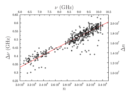
Figure 4: The spacing $\Delta n$ (right axis) of the emission bands shown in Fig. 3 versus their mean harmonic number $n$ (lower axis). The solid line represents the function given in equation (24) for $\Omega/\omega=1.9\times 10^{4}$, $a_{\parallel}=1.03\times 10^{4}$ and $b_{\parallel}=1.48\times 10^{-5}$. The upper axis shows observation frequecy $\nu=n\omega/2\pi$ relevant for the Crab pulsar; the left axis shows $\Delta\nu$. Data points for the Crab pulsar are taken from Fig. 10 of Hankins & Eilek (2007).

It will therefore be seen that the salient parameter responsible for the frequency bands in the Crab pulsar is the ratio $\Omega/\omega=(1.9\pm 0.1)\times 10^{4}$. Using $\omega/2\pi\simeq 30$ Hz relevant for the Crab yields a modulation frequency $\Omega/2\pi\simeq 570$ kHz. A plausible cause for this modulation is plasma oscillations within the pulsar’s atmosphere. A plasma frequency of 570 kHz implies a free-electron density $N_{-}\simeq 4\times 10^{3}~{}{\rm cm}^{-3}$, a value that is consistent with the inferred properties of the atmospheres of neutron stars.

5 Suppression of the emission bands by interference: application to the main pulses of the Crab

We now turn to the main pulses of the Crab pulsar, in which the frequency-banded structure is much less apparent (Hankins & Eilek, 2007). If the components of the electric current within the emitting region (the region in which the rotating distribution pattern of the current approaches the observer with the speed of light and zero acceleration) are such that ${\cal P}_{\parallel}$ and ${\cal P}_{\perp}$ simultaneously contribute towards the value of the field, destructive interference of the contributions with differing polarizations could result in the suppression of the emission bands.

This can be easily seen from equation (19) if we note that, in this case, the radiated power for $n\gg 1$ is proportional to

$$\frac{{\rm d}P_{n}}{{\rm d}\Omega_{P}}\propto{Q_{\hat{\varphi}}}^{2}n^{-1/2}[\cos^{2}(\psi-\gamma_{\parallel})+\kappa(n)\cos^{2}(\psi-\gamma_{\perp})],$$ (31)

where

$$\kappa(n)\equiv\Big{|}\frac{{\bar{s}}_{\varphi}\cos\theta_{P}-{\bar{s}}_{z}\sin\theta_{P}}{{\bar{s}}_{r}}\Big{|}^{2}$$ (32)

is a coefficient that, like $\gamma_{\parallel}$ and $\gamma_{\perp}$, could be expanded into a Taylor series about a local value $n_{0}$ of $n$.

Figure 5 shows the $n$ dependence of the right-hand side of equation (31) for a case in which ${Q_{\hat{\varphi}}}$ decays as $n^{-1}$, $\Omega/\omega=1.9\times 10^{4}$ (as in Figs. 3 and 4), $a_{\parallel}=1.03\times 10^{4}$, $b_{\parallel}=1.48\times 10^{-5}$ (as in Fig. 4), $\gamma_{\perp}=\gamma_{\parallel}+\pi/2$, and $\kappa$ can be approximated by $0.9+0.15(n/n_{0}-1)$ with $n_{0}=2\times 10^{8}$. The emission bands are thus replaced by small-amplitude modulations of the radiation intensity that gradually die out. The behaviour of the radiated power shown in Fig. 5 over the interval $2.7\times 10^{8}\leq n\leq 3.5\times 10^{8}$ is consistent with those of the short-lived microbursts that are observed over the corresponding frequency interval ($8.25$–$10.5$ GHz) within the main pulses of the Crab pulsar [see Figs. 2–4 of Hankins & Eilek (2007)].

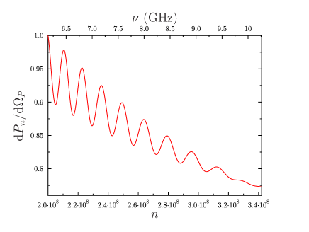
Figure 5: The radiated power ${\rm d}P_{n}/{\rm d}\Omega_{P}$ per harmonic per unit solid angle (in arbitrary units) versus $n$ from a region of the magnetosphere in which the contributions from differing polarizations are comparable in magnitude. The dependence of the right-hand side of equation (31) on $n$ is shown for $Q_{\hat{\varphi}}\sim n^{-1}$, $\gamma_{\perp}=\gamma_{\parallel}+\pi/2$, $\kappa=0.9+0.15(n/n_{0}-1)$, and the same values of $\Omega/\omega$, $a_{\parallel}$, $b_{\parallel}$, and $n_{0}$ as in Fig. 4. The top axis of this Figure gives frequency $\nu$ relevant for observations of the Crab pulsar.

The radiation described by equation (15) would be elliptically polarized if either ${\bar{s}}_{\varphi}$ or ${\bar{s}}_{r}$ is dominant, and linearly polarized if ${\bar{s}}_{z}$ is dominant. The high degree of linear polarization of the interpulse in the frequency range $8.25-10.5$ GHz (Moffett & Hankins, 1999) suggests, therefore, that the interpulse arises from a region of the magnetosphere in which the component of the electric current parallel to the rotation axis dominates, and so the radiation is polarized in the direction of ${\hat{\bf e}}_{\perp}$, while the main pulse arises from a region in which more than one polarization contributes toward the observed field.

This explains not only the difference between the frequency structures of the main pulse and the interpulse, but also the difference between their temporal structures, i.e. the fact that the intensity of the interpulse has a broad and smooth distribution in time, while that of the main pulse is composed of randomly distributed nanoshots (Hankins & Eilek, 2007). It would be possible to identify the individual nondiffracting subbeams described in Sec. 2 only in the case of a source whose length scale of spatial variations is comparable with ${{\hat{R}}_{P}}^{-2}$ (in the case, e.g. of a turbulent plasma with a superluminally rotating macroscopic distribution). The overall beam within which the nonspherically decaying radiation is detectable would then consist of an incoherent superposition of coherent, nondiffracting subbeams with widely differing amplitudes and phases, that would be observed as randomly distributed nanoshots. Otherwise, the smooth transition between the adjacent filamentary parts of the source that generate neighbouring subbeams would result in an overall beam that is likewise smoothly distributed. The filamentary sources sampled from an emitting region in which a single component of the electric current dominates would not be sufficiently different from one another in either amplitude or phase for their associated subbeams to be distinguishable.

The observed difference between the dispersion measures of the main pulse and the interpulse (Hankins & Eilek, 2007) further supports the fact that these pulses arise from distinct regions of the magnetosphere. As we have seen in Sec. 2, an observer who is located at the polar angle $\theta_{P}$ samples, in the course of a rotation, the distribution of the density of the electric current around the cylinder ${\hat{r}}=\csc\theta_{P}$. Thus the profile of the mean pulse reflects the azimuthal distribution pattern of the source.

6 The broadband continuum spectrum of the radiation

Since they only involve a limited range of frequencies, the features of the band emission we have discussed above do not depend on the spectral distributions of the Fourier transforms ${\bar{s}}_{r,\varphi,z}$ of the source densities $s_{r,\varphi,z}$ sensitively. To put the emission bands in the context of the continuum spectrum of the Crab pulsar, however, we would need both a more realistic model of the emitting current distribution and a more explicit description of the dependence of the density of emitting current on frequency. This notwithstanding, the frequencies across which the observed spectrum of the Crab pulsar undergoes sharp changes can be identified with the frequencies at which the Airy function and the coefficients $Q_{\hat{\varphi}}$ and ${\bar{Q}}_{r}$ in the spectrum of the radiation described by equation (15) have their critical points. We have already seen that, for the value $\Omega/\omega=(1.9\pm 0.1)\times 10^{4}$ implied by the observational data of Hankins & Eilek (2007), the position $\Omega^{3}/(\pi\omega^{2})$ of the last peak of the Airy function in equation (15) coincides with the ultraviolet peak in the observed spectrum of the Crab pulsar (Lyne & Graham-Smith, 2006) (Fig. 6).

The coefficient $Q_{\hat{\varphi}}$ in equation (15) is independent of $n$ ($\sim 2\Omega/\omega$) when $n\ll\mu_{+}$, decays as $n^{-1}$ when $n\gg\mu_{+}$, and is of the order of $n$ when $n\simeq m\gg\Omega/\omega$ [see equation(7)]. Hence, if the frequency $m\omega/(2\pi)$ of the azimuthal variations of the source in the Crab pulsar [see equation (1)] falls in the terahertz range, i.e. $m\sim 10^{11}$, then the order of magnitude of $Q_{\hat{\varphi}}$ would change from $\Omega/\omega\sim 10^{4}$ to $n\sim 10^{11}$ across the terahertz gap in its observed spectrum. The corresponding enhancement of the radiated power by a factor of order $(\Delta{Q_{\hat{\varphi}}})^{2}\sim 10^{14}$ is in fact consistent with observational data (see below and Fig. 6). A plausible cause for a frequency $m\omega/2\pi\simeq 3$ THz would be cyclotron resonance of free electrons in a magnetic field of around $10^{6}$ G. A magnetic field of this order at, or close to, the light cylinder, is consistent with the spin-down properties of the Crab pulsar (Lyne & Graham-Smith, 2006).

Moreover, it can be seen from Equations (8) and (9) that the coefficient ${\bar{Q}}_{r}$ changes from being independent of $n$ to decaying as $n^{-1/2}$ when $n$ increases past $\pi{\hat{R}}_{P}/({\hat{r}}_{>}-{\hat{r}}_{<})^{2}$, and so the observation point falls within the Fresnel zone. Given that the Crab pulsar is at the distance $R_{P}\simeq 7.1\times 10^{21}$ cm and has a light cylinder with the radius $c/\omega\simeq 1.6\times 10^{8}$ cm (Lyne & Graham-Smith, 2006), this would account for the corresponding steepening of the observed spectrum of the Crab pulsar at $n\simeq 3\times 10^{16}$ (Fig. 6) if the radial extent of the emitting plasma observed from Earth has the value ${\hat{r}}_{>}-{\hat{r}}_{<}\simeq 6.8\times 10^{-2}$, i.e. $6.8$ percent of the light-cylinder radius.

These generic features of the spectrum of the radiation from a superluminal source, which do not sensitively depend on the detailed distributions of the Fourier components ${\bar{s}}_{r,\varphi,z}$ of the source densities, are adequately described by the following simplified version of equation (15):

$$\frac{{\rm d}P_{n}}{{\rm d}\Omega_{P}}\propto|{\bar{Q}}_{r}|^{2}{Q_{\hat{\varphi}}}^{2}{S(n)}^{2}\left(\frac{2}{n}\right)^{2/3}{\rm Ai}^{2}\left[-\left(\frac{2}{n}\right)^{1/3}\frac{\Omega}{\omega}\right],$$ (33)

where $S(n)$ stands for the dependence of the source density on $n$. For $\Omega/\omega=1.9\times 10^{4}$ and a ${\bar{Q}}_{r}(n)$ that steepens by the factor $n^{-1/2}$ across $n\simeq 3\times 10^{16}$, equation (33) yields the continuum spectrum shown in Fig. 6 if we assume that $S(n)$ dominates over $Q_{\hat{\varphi}}$ everywhere, except across $n=10^{11}$ where $Q_{\hat{\varphi}}$ increases by the factor $10^{14}$ (due to the above-mentioned resonance with $m\omega/2\pi\simeq 3$ THz), and decays as $n^{-3/2}$ in $n<10^{11}$ and as $n^{-1/12}$ in $n>10^{11}$. Note the close correspondence, in Fig. 6, of equation (33) with the observational data on the spectrum of the Crab pulsar over 16 orders of magnitude of frequency (Lyne & Graham-Smith, 2006).

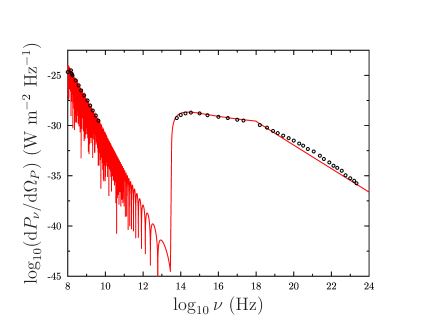
Figure 6: The spectral distribution $\log({\rm d}P_{\nu}/{\rm d}\Omega_{P})$, predicted by equation (33), versus $\log\nu$ for $\nu=n\omega/(2\pi)\simeq 30n$ Hz appropriate for the Crab pulsar. The points show observational data (where available) of the spectrum of the Crab pulsar (Lyne & Graham-Smith, 2006). In the model, the recovery of intensity at the ultraviolet peak at $\sim 10^{15}$ Hz is caused by resonant enhancement due to the azimuthal modulation frequency $m\omega/2\pi\simeq 3$ THz. The change in gradient at $\sim 10^{18}$ Hz reflects a transition across the boundary of the Fresnel zone (see text).

7 Discussion and Summary

We must stress the model-independent nature of the results we have reported here. The only global property of the magnetospheric structure of the Crab pulsar we have invoked is its quasi-steady time dependence: that the cylindrical components $j_{r,\varphi,z}(r,\varphi,z;t)$ of the density of the magnetospheric electric current depend on $\varphi$ only in the combination $\varphi-\omega t$. Not only does this property follow from the observational data (as rigorously shown in Appendices A and B), but it is one that has been widely used in the published literature on pulsars [see, e.g., Mestel et al. (1976)].

Calculating the retarded field that is generated by the Fourier component associated with the frequency $\Omega$ of such a quasi-steady current distribution, we have derived a broadband radiation spectrum with oscillations whose peaks are proportionately spaced in, and decay algebraically with, frequency. By inferring the values of the parameters $\Omega/2\pi\simeq 570$ kHz and $m\omega/2\pi\simeq 3$ THz from the observational data and mildly restricting certain local properties of the source densities ${\bar{s}}_{r,\varphi,z}$ that appear in the derived expression we have quantitatively accounted for the following features in the observed spectrum of the Crab pulsar:

1. the spacing of the emission bands,

2. the frequency at which the extrapolated spacing between these bands would reduce to zero,

3. the widths of the emission bands (their number within a given frequency interval),

4. the salient features of the continuum spectrum (its sharp rise across the terahertz gap, its ultraviolet peak, the change by $1$ of the value of its spectral index at $10^{18}$ Hz), and

5. the differences in the polarizations, dispersion measures, and the time and frequency signatures of the main pulse and the interpulse.

Given that the derived band spacing $\Delta n$ increases as $n^{3/2}$ with the harmonic number $n$ [equations (18) and (24)], we predict that the repetition of the observations of Hankins & Eilek (2007) at higher frequencies would result in a dependence of the band spacing on frequency that has a local slope steeper than $0.058$. There should be $12$ bands within the frequency interval $10$–$20$ GHz, for example, whose spacings would increase with frequency as ${\rm d}\Delta n/{\rm d}n\simeq 0.086$.

The two significant input parameters required to simulate the Crab pulsar’s spectrum are a modulation frequency, $\Omega/2\pi\simeq 570$ kHz, tentatively attributed to plasma oscillations of electrons in the pulsar’s atmosphere and $m\omega/2\pi\simeq 3$ THz, possibly corresponding to cyclotron resonance of electrons in a magnetic field of around $10^{6}$ G. The latter gives rise to the resonant increase in spectral weight in the ultraviolet (Fig. 6).

At this point, it is worth considering briefly the influence of the ratio $\Omega/\omega$ on pulsar spectra in general. Given that typical features of the pulsar’s spectrum scale as $(\Omega/\omega)^{3}$, we might expect that pulsars with slower rotational frequencies (and therefore small values of $\omega$) will have observed spectral intensities weighted towards higher frequencies. By contrast, so-called millisecond pulsars (with large $\omega$) might be expected to have emission concentrated at lower frequencies than the Crab. These predictions seem to be borne out both by Geminga ($\omega/2\pi\simeq 4.5$ Hz), which has emission peaked in the ultra-violet to gamma-ray end of the spectrum, and by millisecond pulsars such as 1937+21 ($\omega/2\pi\simeq 642$ Hz) and 1957+20 ($\omega/2\pi\simeq 622$ Hz), both of which show no emission in the GHz range but strong pulses at radiofrequencies (Lyne & Graham-Smith, 2006).

Furthermore, once it is acknowledged that (as shown in Appendices A and B) the current emitting the observed pulses from pulsars has a superluminally-rotating distribution pattern, the results reported in the published literature on the electrodynamics of superluminal sources (Ardavan, 1998; Ardavan et al., 2003, 2004a, 2007; Schmidt et al., 2007; Ardavan et al., 2008a, b) can be used to explain the extreme values of the giant pulses’ brightness temperature ($\sim 10^{40}$ K) (Ardavan et al., 2007), temporal width ($\sim 1$ ns) and source dimension ($\sim 1$ m) (Ardavan et al., 2008a), as well as the unique characteristics of the average pulses’ polarization (their occurrence as concurrent ‘orthogonal’ modes with swinging position angles and with nearly 100 per cent linear or circular polarization) (Schmidt et al., 2007) and spectra (the range $-4$ to $-2/3$ of their spectral indices and the breadth of their bandwidth, from radio waves to gamma-rays) (Ardavan et al., 2008b).

We conclude by re-emphasizing that all these features of the observed radiation are consequences solely of the fact that the emitting current depends on the coordinate $\varphi$ in the combination $(\varphi-\omega t)$. This constraint may be inferred directly from the simplest observation, that pulsars have a rigidly-rotating radiation distribution, and Maxwell’s equations (see Appendices A and B); it leads to a current distribution with a superluminally rotating pattern at a radius $r>c/\omega$ responsible for the unique features of pulsar emission. The explicit form of the current distribution plays a role only in accounting for the pulse-to-pulse variations of the features discussed above (i.e. for the variable ‘weather’ in the pulsar magnetosphere, not its stable ‘climate’). The plasma processes by means of which the magnetic field of the pulsar couples the rotational motion of the central neutron star to the observationally implied rigid rotation of the distribution pattern of the emitting current have no direct bearing on the results reported in this paper. The salient features of the observational data can be understood in terms of the superluminal emission mechanism without a knowledge of the magnetospheric structure of the pulsar.

8 Acknowledgments

We are grateful to Jean Eilek, Tim Hankins, Jim Sheckard, John Middleditch, Joe Fasel, and Andrea Schmidt for helpful discussions. This work is supported by U.S. Department of Energy Grant LDRD 20080085DR, “Construction and use of superluminal emission technology demonstrators with applications in radar, astrophysics and secure communications”. A.A. also thanks the Royal Society for support.

Appendix A Rigid rotation of the radiation pattern implies a rigid rotation of the source’s distribution pattern

As reflected in the highly stable periodicity of the mean profiles of the pulses detected on Earth, the pulsar radiation field has a rigidly rotating distribution pattern on average. That is to say, the cylindrical components of the received radiation fields ${\bf E}$ and ${\bf B}$ depend on the azimuthal angle $\varphi$ only in the combination $\varphi-\omega t$:

$$E_{r,\varphi,z}(r,\varphi,z;t)=E_{r,\varphi,z}(r,\varphi-\omega t,z,t),$$ (34)

$$B_{r,\varphi,z}(r,\varphi,z;t)=B_{r,\varphi,z}(r,\varphi-\omega t,z,t),$$ (35)

where $(r,\varphi,z)$ are the cylindrical polar coordinates based on the axis of rotation, and $\omega$ is the angular frequency of rotation of the observed radiation pattern. An equivalent statement is that the radiation fields ${\bf E}$ and ${\bf B}$ have a quasi-steady time dependence:

$$\left(\frac{\partial}{\partial t}+\omega\frac{\partial}{\partial\varphi}\right)E_{r,\varphi,z}=0,$$ (36)

and

$$\left(\frac{\partial}{\partial t}+\omega\frac{\partial}{\partial\varphi}\right)B_{r,\varphi,z}=0;$$ (37)

for the general solutions of these partial differential equations are given by the expressions on the right-hand sides of equations (34) and (35).

In the Lorenz gauge, the electromagnetic fields appearing in equation (3) are given by a four-potential $A^{\mu}$ that satisfies the wave equation

$${\bf\nabla}^{2}A^{\mu}-{1\over c^{2}}{\partial^{2}A^{\mu}\over\partial t^{2}}=-{4\pi\over c}j^{\mu},$$ (38)

where $\mu=1,2,3$ designate the Cartesian spatial components ${\bf A}$ and ${\bf j}$ of the potential $A^{\mu}$ and the current density $j^{\mu}$ (Jackson, 1999). The retarded solution to this equation in unbounded space is given by equation (4), i.e. by

$$A^{\mu}({\bf x}_{P},t_{P})=c^{-1}\int{\rm d}^{3}x{\rm d}t\,j^{\mu}({\bf x},t)G({\bf x},t;{\bf x}_{P},t_{P}),$$ (39)

where

$$G({\bf x},t;{\bf x}_{P},t_{P})={\delta(t_{P}-t-R/c)\over R}$$ (40)

is the corresponding Green’s function (Jackson, 1999).

Employing equation (3) to write out $B_{r,\varphi,z}$ in terms of the cylindrical components $A_{r,\varphi,z}$ of the vector potential, we see that the potential also has the time dependence expressed in equations (34)–(37). It follows from $B_{r}=r^{-1}\partial A_{z}/\partial\varphi-\partial A_{\varphi}/\partial z$, for instance, that

$${\cal L}B_{r}={1\over r}{\partial\over\partial\varphi}{\cal L}A_{z}-{\partial\over\partial z}{\cal L}A_{\varphi}.$$ (41)

where ${\cal L}$ stands for the differential operator appearing in equations (36) and (37):

$${\cal L}\equiv{\partial\over\partial t}+\omega{\partial\over\partial\varphi}.$$ (42)

This and the corresponding equations for $B_{\varphi}$ and $B_{z}$ show that equation (37) is satisfied if ${\cal L}A_{r,\varphi,z}=0$, i.e. if $A_{r,\varphi,z}$ depend on $\varphi$ and $t$ only in the combination $\varphi-\omega t$.

On the other hand, the cylindrical components of the vector potential are related to the cylindrical components $j_{r,\varphi,z}$ of the current density via the following spatial part of equation (39):

$$\left[\matrix{A_{r_{P}}\cr A_{\varphi_{P}}\cr A_{z_{P}}\cr}\right]=c^{-1}\int r\,{\rm d}r\,{\rm d}\varphi\,{\rm d}z\,{\rm d}t\,G$$ (43)

$$\times\left[\matrix{\cos(\varphi_{P}-\varphi)j_{r}+\sin(\varphi_{P}-\varphi)j_{\varphi}\cr\cos(\varphi_{P}-\varphi)j_{\varphi}-\sin(\varphi_{P}-\varphi)j_{r}\cr j_{z}\cr}\right].$$

Applying the operator

$${\cal L}_{P}\equiv{\partial\over\partial t_{P}}+\omega{\partial\over\partial\varphi_{P}}$$ (44)

to both sides of equation (43) and making use of the fact that $G$ depends on $\varphi_{P}$ and $t_{P}$ in the combinations $\varphi_{P}-\varphi$ and $t_{P}-t$ [equation (40)], and so ${\cal L}_{P}G=-{\cal L}G$, we find that the resulting equation can be cast in the form

$${\cal L}_{P}\left[\matrix{A_{r_{P}}\cr A_{\varphi_{P}}\cr A_{z_{P}}\cr}\right]=c^{-1}\int r\,{\rm d}r\,{\rm d}\varphi\,{\rm d}z\,{\rm d}t\,G$$ (45)

$$\times\left[\matrix{\cos(\varphi_{P}-\varphi){\cal L}j_{r}+\sin(\varphi_{P}-\varphi){\cal L}j_{\varphi}\cr\cos(\varphi_{P}-\varphi){\cal L}j_{\varphi}-\sin(\varphi_{P}-\varphi){\cal L}j_{r}\cr{\cal L}j_{z}\cr}\right]$$

by means of integrations by parts with respect to $\varphi$ and $t$. Hence, ${\cal L}A_{r_{P},\varphi_{P},z_{P}}$ vanishes if and only if ${\cal L}j_{r,\varphi,z}$ is zero.

It follows from equations (42) and (45), therefore, that a necessary and sufficient condition for the rigid rotation of the distribution pattern of the radiation field, i.e. ${\cal L}B_{r_{P},\varphi_{P},z_{P}}=0$, is the corresponding rigid rotation ${\cal L}j_{r,\varphi,z}=0$ of the distribution pattern of the source density.

Appendix B Rigid rotation of the source’s distribution pattern extends beyond the light cylinder

Our purpose here is to show that a solution of Maxwell’s equations that has the quasi-steady time dependence

$$\frac{\partial}{\partial t}+\omega\frac{\partial}{\partial\varphi}=0,$$ (46)

i.e. has a rotating distribution pattern, applies either to the entire magnetosphere or to an expanding region whose boundary propagates at the speed of light. By considering the initial-boundary-value problem for the wave equation (38) with Cauchy data satisfying equation (46), we establish that such a solution cannot be smoothly matched to other types of solutions of Maxwell’s equations across a boundary that is confined to a localized region of the magnetosphere.

The change of variables

$$\xi_{1}=r,\quad\xi_{2}=z,\quad\xi_{3}=\varphi-\omega t,\quad\xi_{4}=\psi(r,\varphi,z,t),$$ (47)

where $\psi$ is, for the moment, to be considered an arbitrary function, transforms the $z$-component of the wave equation (38) into

$$\frac{1}{\xi_{1}}\left(\xi_{1}\frac{\partial A_{z}}{\partial\xi_{1}}\right)+\frac{\partial^{2}A_{z}}{\partial{\xi_{2}}^{2}}+\left(\frac{1}{{\xi_{1}}^{2}}-\frac{\omega^{2}}{c^{2}}\right)\frac{\partial^{2}A_{z}}{\partial{\xi_{3}}^{2}}$$ (48)

$$+\left(|\nabla\psi|^{2}-\frac{1}{c^{2}}{\psi_{t}}^{2}\right)\frac{\partial^{2}A_{z}}{\partial{\xi_{4}}^{2}}+2\psi_{r}\frac{\partial^{2}A_{z}}{\partial\xi_{1}\partial\xi_{4}}$$

$$+2\psi_{z}\frac{\partial^{2}A_{z}}{\partial\xi_{2}\partial\xi_{4}}+2\left(\frac{1}{r^{2}}\psi_{\varphi}+\frac{\omega}{c^{2}}\psi_{t}\right)\frac{\partial^{2}A_{z}}{\partial\xi_{3}\partial\xi_{4}}$$

$$+\left(\nabla^{2}\psi-\frac{1}{c^{2}}\psi_{tt}\right)\frac{\partial A_{z}}{\partial\xi_{4}}=-\frac{4\pi}{c}j_{z},$$

where $\psi_{t}\equiv\partial\psi/\partial t$, $\psi_{r}\equiv\partial\psi/\partial r$, etc. The Jacobian of the above transformation is

$$\frac{\partial(\xi_{1},\xi_{2},\xi_{3},\xi_{4})}{\partial(r,z,\varphi,t)}=\frac{\partial\psi}{\partial t}+\omega\frac{\partial\psi}{\partial\varphi},$$ (49)

which remains non-zero as long as $\psi$ is not a function that depends on $\varphi$ and $t$ as in $\varphi-\omega t$.

Now suppose that at a given time $t$ the surface $\psi(r,\varphi,z,t)=0$ represents the boundary of a region within which the solution to equation (48) satisfies the symmetry (46), i.e. within which $A_{z}$ is a function of $\xi_{1}$, $\xi_{2}$ and $\xi_{3}$ only. At all points on this boundary, we then have

$$\frac{\partial A_{z}}{\partial\xi_{4}}\bigg{|}_{\xi_{4}=0}=0$$ (50)

and

$$\frac{1}{\xi_{1}}\frac{\partial}{\partial\xi_{1}}\left(\xi_{1}\frac{\partial A_{z}}{\partial\xi_{1}}\right)+\frac{\partial^{2}A_{z}}{\partial{\xi_{2}}^{2}}$$ (51)

$$+\left(\frac{1}{{\xi_{1}}^{2}}-\frac{\omega^{2}}{c^{2}}\right)\frac{\partial^{2}A_{z}}{\partial{\xi_{3}}^{2}}+\frac{4\pi}{c}j_{z}\bigg{|}_{\xi_{4}=0}=0,$$

where (51) is the wave equation under symmetry (46); (50) and (51) hold at the boundary of the region in question by virtue of holding inside that region.

Hence, any other type of solution of the wave equation that would match the symmetric solution across $\psi=0$ smoothly has to be sought by solving the following initial-value problem: given that the Cauchy data on the hypersurface $\xi_{4}=0$ are those expressed in (50) and (51), what is the solution to the hyperbolic partial differential equation (48) beyond $\xi_{4}=0$? Note that since $\partial A_{z}/\partial\xi_{4}$ vanishes at all points of the hypersurface $\xi_{4}=0$, its derivatives $\partial^{2}A_{z}/\partial\xi_{1}\xi_{4}$, $\partial^{2}A_{z}/\partial\xi_{2}\xi_{4}$ and $\partial^{2}A_{z}/\partial\xi_{3}\xi_{4}$, which are in directions interior to this hypersurface, also vanish at $\xi_{4}=0$.

Thus, equation (48) in conjunction with the data (50) and (51) demands that

$$\left(|\nabla\psi|^{2}-\frac{1}{c^{2}}{\psi_{t}}^{2}\right)\frac{\partial^{2}A_{z}}{\partial{\xi_{4}}^{2}}\bigg{|}_{\xi_{4}=0}=0.$$ (52)

There are two ways in which this requirement could be met: either $\psi=0$ is a characteristic surface of the wave equation, and hence the first factor in (52) vanishes, or at $\psi=0$ the derivative of $\partial A_{z}/\partial\xi_{4}$ in the direction normal to the boundary is also zero. In the first case, the boundary of the domain in which symmetry (46) is satisfied, $\psi=0$, will consist of an expanding wave front that propagates at speed $c$. In the second case, the solution outside $\psi=0$ will also be symmetric, according to the Cauchy-Kowalewski theorem [cf. Courant & Hilbert (1962)]. This is because the extension (by means of a Taylor series) of the data into an integral strip next to the boundary $\psi=0$ will yield a solution that is again independent of $\xi_{4}$. Since the above argument applies also to the new boundary of the region thus extended, it follows that $A_{z}$ will also be be independent of $\xi_{4}$ outside the surface $\psi(r,\varphi,z,t)=0$, i.e. will be a function of $(r,\varphi-\omega t,z)$ throughout the magnetosphere.

The corresponding results for $A_{r}$ and $A_{\varphi}$ may be derived in the same way.

Appendix C Asymptotic expansion of the spectrum for high radiation frequencies

In this Appendix, we evaluate the leading term in the asymptotic expansion of the Anger functions that appear in equation (6) for a radiation frequency ($n\omega$) that appreciably exceeds both the rotation ($\omega$) and modulation ($\Omega$) frequencies of the source, though not necessarily the frequency $m\omega$ of its spatial oscillations.

In this regime, the Anger functions ${\bf J}_{n-\Omega/\omega}(n)$ and ${{\bf J}^{\prime}}_{n-\Omega/\omega}(n)$ can be approximated by the Bessel functions $J_{n-\Omega/\omega}(n)$ and ${J^{\prime}}_{n-\Omega/\omega}(n)$, respectively [see equation (41) of Ardavan et al. (2003)]. Once we cast these Bessel functions into the canonical forms $J_{\mu}(\mu+\zeta\mu^{1/3})$ and ${J^{\prime}}_{\mu}(\mu+\zeta\mu^{1/3})$ by introducing the new variables

$$\mu\equiv n-\frac{\Omega}{\omega},\qquad\qquad\zeta\equiv\frac{\Omega}{\omega}\left(n-\frac{\Omega}{\omega}\right)^{-1/3},$$ (53)

we can write the leading terms in their asymptotic expansions for large $\mu$ as

$$J_{\mu}(\mu+\zeta\mu^{1/3})\simeq(2/\mu)^{1/3}{\rm Ai}(-2^{1/3}\zeta),$$ (54)

and

$${J^{\prime}}(\mu+\zeta\mu^{1/3})\simeq-(2/\mu)^{2/3}{\rm Ai}^{\prime}(-2^{1/3}\zeta)$$ (55)

[see equations (9.3.23), (9.3.27) of Abramowitz & Stegun (1970)]. Taking the limits $n\gg\Omega/\omega$ of the coefficients and arguments of the above Airy functions, we obtain the expressions in equations (13) and (14).

For $(\Omega/\omega)\ll n\ll(\Omega/\omega)^{3}$, the argument of the resulting Airy function and its derivative that appear in equations (13) and (14) is large, so that we can further use the asymptotic approximations

$${\rm Ai}(-\chi)\simeq\pi^{-1/2}\chi^{-1/4}\cos(\textstyle{2\over 3}\chi^{3/2}-\pi/4),$$ (56)

and

$${\rm Ai}^{\prime}(-\chi)\simeq\pi^{-1/2}\chi^{1/4}\sin(\textstyle{2\over 3}\chi^{3/2}-\pi/4),$$ (57)

[see equations (10.4.60) and (10.4.62) of Abramowitz & Stegun (1970)] to replace them by the trigonometric functions given in equations (16) and (17).

Note that if $\Omega$ is replaced by $-\Omega$, the argument of the above Airy functions assume a positive value, and hence the resulting Anger functions ${\bf J}_{n+\Omega/\omega}(n)$ and ${{\bf J}^{\prime}}_{n+\Omega/\omega}(n)$ decay exponentially, rather than algebraically, with increasing $n$ [see Abramowitz & Stegun (1970)].

References

- Abramowitz & Stegun (1970) Abramowitz M., Stegun I.A., 1970, Handbook of Mathematical Functions (Dover)
- Ardavan (1998) Ardavan H., 1998, Phys Rev E, 58, 6659
- Ardavan et al. (2003) Ardavan H., Ardavan A., Singleton J., 2003, J Opt Soc Am A, 20, 2137
- Ardavan et al. (2004a) Ardavan H., Ardavan A., Singleton J., 2004a, J Opt Soc Am A, 21, 858
- Ardavan et al. (2004b) Ardavan A., Hayes W., Singleton J., Ardavan H., Fopma J., Halliday D., 2004b, J Appl Phys, 96, 7760
- Ardavan et al. (2007) Ardavan H., Ardavan A., Singleton J., Fasel J., Schmidt, A., 2007, J Opt Soc Am A, 24, 2443
- Ardavan et al. (2008a) Ardavan H., Ardavan A., Singleton J., Fasel J., Schmidt A., 2008a, J Opt Soc Am A, 25, 543
- Ardavan et al. (2008b) Ardavan H., Ardavan A., Singleton J., Fasel J., Schmidt A., 2008b, J Opt Soc Am A, 25, 780
- Bessarab et al. (2004) Bessarab A.V., Gorbunov A.A., Martynenko S.P., Prudkoy N.A., 2004, IEEE Trans Plasma Sci, 32, 1400
- Bolotovskii & Ginzburg (1972) Bolotovskii B.M., Ginzburg V.L., 1972, Sov Phys Usp, 15, 184
- Bolotovskii & Bykov (1990) Bolotovskii B.M., Bykov V.P., 1990, Sov Phys Usp, 33, 477
- Bolotovskii & Serov (2005) Bolotovski B.M., Serov A.V., 2005, Phys Usp, 43, 903
- Courant & Hilbert (1962) Courant R., Hilbert D., 1962, Methods of Mathematical Physics, Vol. II (Interscience)
- Ginzburg (1972) Ginzburg V.L., 1972, Sov Phys JETP, 35, 92
- Gold (1968) Gold T., 1968, Nature, 218, 731
- Goldreich & Julian (1969) Goldreich P., Julian W.H., 1969, Ap J, 157, 869
- Hankins et al. (2003) Hankins T.H., Kern J.S., Weatherall J.C., Eilek J.A., 2003, Nature, 422, 141
- Hankins & Eilek (2007) Hankins T.H., Eilek J.A., 2007, Ap J, 670, 693
- Jackson (1999) Jackson J.D., 1999, Classical Electrodynamics, 3rd ed. (Wiley)
- Lyne & Graham-Smith (2006) Lyne A.G., Graham-Smith F., 2005, Pulsar Astronomy (Cambridge U Press)
- Mestel et al. (1976) Mestel L., Wright G.A.E., Westfold K.C., 1976, MNRAS, 175, 257
- Moffett & Hankins (1999) Moffett D.A., Hankins T.H., 1999, ApJ, 522, 1046
- Schmidt et al. (2007) Schmidt, A., Ardavan H., Fasel J., Singleton J., Ardavan A., 2007, Proceedings of the 363rd WE-Heraeus Seminar on Neutron Stars and Pulsars, eds. Becker W., Huang H.H., 124
- Singleton et al. (2004) Singleton J., Ardavan A., Ardavan H., Fopma J., Halliday D., Hayes W., 2004, in Digest of the 2004 Joint 29th International Conference on Infrared and Milimeter Waves and 12th International Conference on Terahertz Electronics (IEEE), 591
- Soglanov et al. (2004) Soglanov V.A., Popov M.V., Bartel N., Cannon W., Novikov A.Y., Kondratiev V.I., Altunin V.I., 2004, Ap J, 616, 439