Wave-breaking and generic singularities of nonlinear hyperbolic equations

Abstract

Abstract Wave-breaking is studied analytically first and the results are compared with accurate numerical simulations of 3D wave-breaking. We focus on the time dependence of various quantities becoming singular at the onset of breaking. The power laws derived from general arguments and the singular behavior of solutions of nonlinear hyperbolic differential equations are in excellent agreement with the numerical results. This shows the power of the analysis by methods using generic concepts of nonlinear science.

I Introduction

Among the myriad of natural phenomena dominated by nonlinearity, wave-breaking is quite special. It is ubiquitous along most oceanic shorelines, and although progress has recently been made in its understanding, its full explanation remains somewhat shrouded in mystery. This makes wave-breaking an outstanding topic in the study of nonlinear phenomena and, we believe, one that is particularly well suited to this “Open problems section of Nonlinearity”. Wave-breaking also plays a significant role in the larger scale dynamics of the Oceans dias , particularly with respect to their interaction with the atmosphere. For instance, the swell provides nucleation seeds for the rain and wind momentum exchange with water, mostly through nonlinear processes. Among such processes, wave-breaking could also be significant, if not dominant, to limit the growth of the instability responsible of the formation of waves.

The linear theory of waves has a long and interesting history, going back to the Principia. In book 2 Newton shows that the velocity of water waves in the infinite depth limit is proportional to $\sqrt{g\lambda}$, with $g$ the acceleration of gravity and $\lambda$ the wavelength. Years later, Bernoulli derived the shallow water wave velocity, applicable to waves with a wavelength much larger (typically more than 20 times) than the water depth. The interpolation between these two limits is due to Lagrange. Later, in a very important paper, Stokes defined the range of applicability of the linear theory in the shallow water limit. Thereafter Riemann’s method of solution of quasilinear equations showed the occurrence of a finite time singularity for simple waves in the shallow water case. Among the open problems posed by the occurrence of such a singularity, we shortly discuss below the two existing methods proposed to regularize the wave profile to avoid the occurrence of an overhang. These methods introduce the next order space derivative in the shallow water equations (i.e., so-called dispersive effects) and thus preclude wave-breaking from occurring.

The relationship between wave-breaking and the nonlinear structure of the governing equations is reconsidered below, where we show that strong nonlinearities dominate the wave dynamics, both in the transverse and longitudinal directions. Starting from generic equations, whose solution can develop discontinuities (inviscid Burgers, or pressure-less fluid equations), we first show in a one-dimensional space (1D), that a very simple (once known as Poisson ) solution $u(x,t)$ of this partial differential equation does yield a wave-breaking (i.e., overturning) process. Defining $u$ as the free surface elevation, we study its dynamical behavior and, more specifically, the growth of the overhang domain with time.

Extending the pressure-less fluid equation to a two-dimensional space (2D), we obtain a generic equation for $u(x,y,t)$ showing how the “overhanging domain” of the overturning wave extends in both spatial directions, parallel and normal to the wave. In that case, the boundary of the overhanging region, referred to as the “apparent contour” (i.e., the set of points where the tangent to the water surface is vertical), becomes a skewed curve, when drawn on the water surface. We find that this curve spreads as $t^{3/2}$ in the direction of wave propagation and as $t^{1/2}$ along the wave crest ($t=0$ being the instant where wave overturning is initiated, yielding an overhanging region). These results will be shown to be in good agreement with those of numerical simulations of a 3D overturning wave over a sloping underwater ridge, based on the solution of Euler equations with free surface boundary conditions GG . Moreover the lateral spreading as $t^{1/2}$ was recently found experimentallymarseille for waves generated by a wave-maker, and progressing on an horizontal bottom.

These time evolution laws are established first for a pressure-less fluid and then are extended in section III to the shallow water case. The scaling laws for wave-breaking, in the directions perpendicular and parallel to the crest, will be derived from solutions of fluid-mechanical equations. It is true that this wave-breaking process could be seen as an example of a metamorphosis of a surface studied in catastrophe theory, named a ’sickle’ or ’lips’. In particular, Arnold arnold , referring to physical situations completely different of ours, notices that the width of a ’sickle’ should grow generically like $(t-t_{0})^{1/2}$, $t_{0}$ being the time of the first singularity. This law of growth is the same as the one we find for the lateral spreading of the overturning domain. However catastrophe theory is very general and cannot be considered as providing any kind of mathematical method for solving the equations of fluid mechanics. Therefore we did not feel useful to use this theory explicitly in the present work and we relied instead on explicit solutions of the fluid equations. Moreover, to the best of our knowledge, catastrophe theory has never been used in investigations of the wave-breaking problem. This being a contribution to the Open problems section of the Journal, in section 4 we comment on various aspects of the problem that do wander off the main track. For instance, we suggest an extension of the boundary integral method (e.g., such as used in GG ) to deal with the wave-breaking problem, beyond the time when the plunging jet impinges on the free surface underneath, and briefly discuss some features of what we call the Hertz-fluid contact problem.

II From 1D to 2D wave-breaking

In this section, we first introduce a generic singular solution to a nonlinear hyperbolic partial differential equation (PDE), in a one-dimensional space (1D). We then show that such solutions of the PDE can be represented by a curve that is continuously deforming and, hence, can be used as a simple geometric model for predicting the occurrence of an overhanging region, similar to the plunging jet in an overturning (i.e., breaking) water wave. We finally extend this equation to a two-dimensional space (2D), which is a more physically relevant case.

II.1 Wave-breaking in one dimension

Consider the equation

$$\frac{\partial u}{\partial t}+u\frac{\partial u}{\partial x}=0\mathrm{.}$$ (1)

It has Poisson the implicit solution

$$u(x,t)=u_{0}(x-ut)\mathrm{,}$$ (2)

where $u_{0}(x)$ is the initial condition. Let $f(.)$ be the inverse function of $u_{0}(.)$ (all functions assumed smooth). Therefore:

$$f(u(x,t))=x-ut\mathrm{.}$$ (3)

This solution $u(x,t)$, as given by equation (3), becomes multivalued whenever $\frac{\partial x}{\partial u}=0$, the derivative being taken at constant $t$. From equation (3), this yields

$$t+\frac{{\mathrm{d}}f}{{\mathrm{d}}u}=0\mathrm{.}$$ (4)

The smallest $t$ when this has a root, for a given $f(u)$, is when this root is stationary with respect to $t$, that is when ${\mathrm{d}}t=0$, with $t$ and $u$ related by (4). This yields ${\mathrm{d}}t=-{\mathrm{d}}u\frac{{\mathrm{d}}^{2}f}{{\mathrm{d}}u^{2}}=0$, or simply $\frac{{\mathrm{d}}^{2}f}{{\mathrm{d}}u^{2}}=0$. Therefore, at the singularity, $f$ has a vanishing second derivative, a standard result. Furthermore it can also be assumed that the Taylor series expansion (TSE) of $f$ has no linear term (amounting to take $u=0$ as the value of $u$ where $f(.)$ has an inflection point), since a constant $u$ can be absorbed into a redefinition of the time origin in equation (3). Let us then define $t=0$ as the first time when the solution becomes singular, to avoid having to write $(t-t^{*})^{3/2}$ etc. instead of $t^{3/2}$, with $t^{*}$ time of the singularity. Near the singularity (assumed to occur at $t=0$) one can thus expand (after convenient scaling)$f(u)$ like $f(u)=-u^{3}+au^{4}+...$, with $a$ finite constant. Once put into equation (3) this gives to the 4th-order:

$$au^{4}=u^{3}+x-ut\mathrm{.}$$ (5)

For short times , Equation (5) implies that $u$ scales like $t^{1/2}$ and $x$ like $t^{3/2}$, which makes all terms on the right-hand side of Equation (5) of the same order, $t^{3/2}$. The left-hand side term is - with the same scaling law - of order $t^{2}$ and therefore negligible compared to the right-hand side; this applies as well to higher-order terms in the TSE of $f(u)$ near the inflection point. Assuming that the beginning of an overhanging region can be described by the lower-order terms, the ’universal’ equation describing ’wave-breaking’ reads:

$$0=u^{3}+x-ut\mathrm{.}$$ (6)

Note that, in this derivation, the coefficient of $u^{3}$ of the TSE of $f(u)$ near zero is negative and thus a singularity will appear for positive times. For negative times, Equation (6) only has one real root while it has three such roots for positive times.

Therefore the curve $u(x,t)$ is everywhere single-valued if its slope is negative at $x=0$, which happens for $t$ negative. By contrast, $u(x,t)$ is triple-valued in a range of values of $x$, if $t$ is positive. This solution can be put in a self-similar form by eliminating one variable. The scaling laws for the transition from single to triple-valued results are $u\sim\sqrt{|t|}$ and $x\sim|t|^{3/2}$. Therefore, the ’natural’ solution of Equation (5) is of the form $u(x,t)=\sqrt{|t|}U(\zeta)$, with $\zeta=x|t|^{-3/2}$ and $U$ a numerical function. Nevertheless, this is not sufficient, because the function $U(.)$ takes different values depending on whether $t$ is negative, zero, or positive. This can be taken into account formally by introducing a discrete argument in the function $U(.)$, namely an index $i$ with three possible values $-1$, $0$ and $1$, such that $i=-1$ if $t$ is negative, $i=0$ if $t=0$ and $i=1$ if $t$ is positive. This defines three real numerical functions $U_{i}(\zeta)$, such that $U_{-1}(\zeta)$ is the real root of $0=U_{-1}^{3}+\zeta+U_{-1}$, and $U_{0}=-\zeta^{1/3}$. The multivalued function $U_{1}$ is any real root of $0=U_{1}^{3}+\zeta-U_{1}$, with three possible values in the range $-\frac{2\sqrt{3}}{3}<\zeta<\frac{2\sqrt{3}}{3}$ and one otherwise.

This completely defines the self-similar solution.

II.2 Wave-breaking in more than one space dimension

Our approach to the formation of singularities in solutions of hyperbolic equations can be extended to nonlinear differential equations with more than one spatial variable. A simple extension of the nonlinear equation (1) provides a model for the occurrence of singularities for time-dependent functions of two coordinates of space $(x,y)$. Let $u(x,y,t)$ and $v(x,y,t)$ be the two Cartesian horizontal components of the velocity field of a fluid, with $(x,y)$ the horizontal coordinates and $x$ in the direction of propagation. Momentum equations, without pressure or gravity read:

$$\left\{\begin{array}[]{l}\frac{\partial u}{\partial t}+u\frac{\partial u}{\partial x}+v\frac{\partial u}{\partial y}=\epsilon\nabla^{2}u\\ \frac{\partial v}{\partial t}+u\frac{\partial v}{\partial x}+v\frac{\partial v}{\partial y}=\epsilon\nabla^{2}v\mathrm{,}\end{array}\right.$$ (7)

with $\epsilon$ a viscosity coefficient. Note that mathematical models with a similar formalism have been proposed zeldo to describe the formation of large scale structures in the Universe, assuming a potential flow, namely that a function $\Phi(x,y)$ exists such that $u=-\frac{\partial\Phi}{\partial x}$ and $v=-\frac{\partial\Phi}{\partial y}$. Such a dependence of the velocity field on a potential is possible for the present model: if the flow is potential at $t=0$, equations (7) reduce to the unsteady Bernoulli equation, which ensures that the flow remains potential for all times. In this potential flow case, equations with the viscous terms can still be solved thanks to Florin’s florin transform (often referred to as Hopf-Cole transform) : $S=-2\epsilon\ln|\Phi|$ , which yields a linear diffusion equation for $S(x,y,t)$.

For $\epsilon=0$ equations(7) have the formal solution very similar to equation (3):

$$\left\{\begin{array}[]{l}x-tu(x,y,t)=F(u,v)\\ y-tv(x,y,t)=G(u,v)\mathrm{}\end{array}\right.$$ (8)

where the functions $F,G$ are presented below. Let $M$ be the general two-by-two matrix of the linear group, with non-zero determinant. Therefore $(\tilde{u},\tilde{v})=M(u,v)$ and $(\tilde{x},\tilde{y})=M(x,y)$ are solutions of equations of the same form as the left-hand side of Equation (8). This holds true with the same matrix acting on $(u,v)$ and $(x,y)$. The same general linear map will change in general the functions $F(u,v)$ and $G(u,v)$ in a rather complicated way. However because the map is linear it will not change the degree of a polynomial in $u$ and $v$. Based on that property, we shall be able to show, almost without any calculation, that singularities yielding discontinuities of derivatives with respect to $x$ may spread in any direction, the analysis being made by assuming first that the singularity spreads normal to $x$.

The functions $F(u,v)$ and $G(u,v)$ are defined by the initial conditions. For smooth initial data they are such that the mapping from $(u,v)$ to $(x,y)$, defined by $x=F(u,v)$ and $y=G(u,v)$ is one to one. Therefore the Jacobian $J(t=0)=\frac{\partial G}{\partial v}\frac{\partial F}{\partial u}-\frac{\partial G}{\partial u}\frac{\partial F}{\partial v}$ never vanishes. The solution of equations (8) becomes singular whenever the time-dependent Jacobian $J(t)$ of the mapping of $(u,v)$ onto $(x,y)$ becomes singular. This Jacobian reads :

$$J(t)=\left(\frac{\partial G}{\partial v}+t\right)\left(\frac{\partial F}{\partial u}+t\right)-\frac{\partial G}{\partial u}\frac{\partial F}{\partial v}\mathrm{.}$$ (9)

Let us assume that the singularity first occurs at $t=0$ and $x=y=0$, with $u=v=0$ as well. The latter restriction is not as important as one could believe at first : the original equations are Galilean invariant, so that one can always specify that the velocity field is $u=v=0$ at some point of time and space.

The condition equivalent to the cancelation in 1D of the second derivative of $f(u)$ at $u=0$, here, is the property that, near $t=u=v=0$, the first relevant terms in the TSE of the Jacobian $J(t)$ read

$$J(t)=at+bu^{2}+cv^{2}+2duv\mathrm{,}$$ (10)

where $a$, $b$, $c$ and $d$ are constant derived from the TSEs of $F(u,v)$ and $G(u,v)$ near zero. The expansion (10) implies that there is no term linear with respect to $u$ and $v$. Otherwise the Jacobian would vanish for $t$ negative and for small values of $u$ and $v$, which is not the case based on our assumptions. The two coefficients of the part of the Jacobian linear with respect to $u$ and $v$ vanish generically at points in the $(x,y)$ plane. Of course, besides this cancelation, there are constraints on the sign of $a$ and of the quadratic form $bu^{2}+cv^{2}+2duv$ to make the singularity appear as time increases. For instance, if $a$ is positive, the quadratic form $bu^{2}+cv^{2}+2duv$ must be negative definite, which requires $c$ and $b$ negative and $d^{2}-ab$ negative.

The functions $F(u,v)$ and $G(u,v)$ have to be expanded in Taylor series at least to third-order to yield the quadratic term $bu^{2}+cv^{2}+2duv$ in the Jacobian. This depends on two sets of eight coefficients. Fortunately this calculation is greatly simplified by limiting oneself to the quantities at leading order near $t=0$. The Jacobian at leading order depends on the linear terms in the TSE of $F$ and $G$ near $u=v=0$. Let us note that coordinates $x$ and $y$ do not have to be taken in directions orthogonal to each other, because the Jacobian matrix is reduced to its diagonal form by a general change of coordinates that is not necessarily a rotation, the Jacobian matrix having no reason to be real symmetric in general. At $t=0$ the Jacobian matrix has a zero eigenvalue, that can always be associated with an eigenvector pointing in the $x$ direction. Therefore the coefficients of the TSE of $F(u,v)$ and $G(u,v)$ have to satisfy the condition that $\frac{\partial F}{\partial u}=0$, $\frac{\partial F}{\partial v}=0$ and $\frac{\partial G}{\partial u}=0$ at $u=v=0$. This yields that, near the singularity, one has at leading order

$$\left\{\begin{array}[]{l}F(u,v)=b^{\prime}v^{2}+d^{\prime}u^{3}\\ G(u,v)=c^{\prime}v\mathrm{,}\end{array}\right.$$ (11)

with $b^{\prime},c^{\prime}$ and $d^{\prime}$ coefficients depending on the initial conditions for the original equation, which are related to the constant $a,b$ of expansion (10) by the relation $a=c^{\prime}$, $b=3c^{\prime}d^{\prime}$. Therefore at leading order, the second equation (8) writes

$$y=c^{\prime}v\mathrm{,}$$ (12)

because one can neglect the term $vt$ as compared to $c^{\prime}v$ (because $t$ is a priori much smaller than the constant $c^{\prime}$, assumed non-zero). The first equation (8) becomes:

$$x-\frac{b^{\prime}}{c^{\prime 2}}y^{2}-ut=d^{\prime}u^{3}\mathrm{.}$$ (13)

This equation is not yet the one we are aiming for, because it describes a singularity all along the parabola of Cartesian equation $x-\frac{b^{\prime}}{c^{\prime 2}}y^{2}=0$ at time $0$. Actually we omitted a term of order $uv^{2}$ in the TSE of $F(u,v)$. Let us thus write $F(u,v)=b^{\prime}v^{2}+d^{\prime}u^{3}+g^{\prime}uv^{2}$. The term $g^{\prime}uv^{2}$ ultimately yields a term of order $y^{2}u$ in the equation for $u$. Contrary to the term $-\frac{b^{\prime}}{c^{\prime 2}}y^{2}$ just considered, this one changes the singularity completely in the sense that, with this term, the singularity occurs first at a point in the $(x,y)$ plane and later spreads in the $y$ direction. Thus, after some elementary rescaling, equation (6) for the 1D case is changed into:

$$0=u^{3}+x-\beta y^{2}-u(t-y^{2})$$ (14)

which is the main result of this section.

Note, we neglected the term $m^{\prime}u^{2}v$ in the TSE of $F(u,v)$, although it is of the same order of magnitude, $|t|^{3/2}$, as the one we kept. This is because this term yields a term like $u^{2}y$ in the equation for $u$, which can be eliminated by redefining $u$ as $u+m"y$, with $m"=\frac{m^{\prime}}{3}$, a constant. Also, first, note that for actual overturning waves in shallow water, at least at leading order, the velocity component $u$ is proportional to the surface elevation (see section 4 where simple waves are defined for this case). From now on, let us consider $u$ as the surface elevation, until we can further define the elevation origin. Second, note that in equation (14), the term $-\beta y^{2}$ changes the support of the singularity from a straight line to a bent line. Additionally, except for this term, all other terms in equation (14) are of order $|t|^{3/2}$ near the singularity, with

$$y\sim|t|^{1/2},u\sim|t|^{1/2},x\sim|t|^{3/2}\mathrm{.}$$ (15)

Now, for a given value of $t$, the extension of the overhanging region of the 3D surface $u(x,y,t)$ may be visualized by the set of points where the tangent plane is vertical; this set of points will be referred to as the apparent contour $\it{C_{v}}$. Differentiating equation (14), we get the relation $(3u^{2}+y^{2}-t)du+dx+(2u-2\beta)dy=0$. Along $\it{C_{v}}$, the condition of a vertical tangent, i.e., infinite values of partial derivatives ($\frac{\partial u}{\partial x}$, $\frac{\partial u}{\partial y}$), requires that the coefficient of the $du$ term vanish. Introducing the relation $3u^{2}+y^{2}-t=0$ into equation (14), yields the equation for the apparent contour,

$$x=\beta y^{2}\pm\frac{2}{3^{3/2}}(t-y^{2})^{3/2}\mathrm{.}$$ (16)

Figure 1: Boundary of the overhanging region or apparent contour $\it{C_{v}}$, given by equation (14), with $\beta=-0.5$. Leftward figure : just after the beginning of the overturning process at $t=0.13$; rightward figure : for $t=1.4$, which is actually beyond the range of validity of the ’generic equation’

.

Equation (16) is plotted in Fig. (1), and shows the boundary of the overhanging domain projected on the horizontal plane, at time $t$ after the inception of the singularity. This boundary spreads along the parabolic curve of Cartesian equation $x=\beta y^{2}$. The width of the crescent shaped boundary expands as $x\sim|t|^{3/2}$, while its length expands as $y\sim|t|^{1/2}$.

These analytical predictions are compared in the next section to results of numerical simulations of wave-breaking, derived from those reported in GG .

II.3 Numerical simulation of wave-breaking

Euler equations with fully nonlinear free surface conditions have recently been solved numerically in 3D, to simulate the early stages of solitary wave-breaking induced by changes in topography in shallow water, namely a curved sloping ridge GG . Note that the word ”solitary” refers here to a single, isolated wave, not to a soliton-like wave propagating without changing shape. The flow in the initial solitary wave being irrotational, Kelvin theorem implies that this will be the case for any positive value of $t$. Hence, the problem is described by fully nonlinear potential flow equations, which are solved in the model with a high-order boundary element method, combined with an explicit time-integration method, expressed in a mixed Euler-Lagrangian formulation. In fact, earlier comparisons of 2D numerical results with laboratory experiments have shown that the full potential theory predicts well wave overturning in deep water, as well as wave shoaling and overturning over slopes Grilli . Recent contributions to 3D simulations of nonlinear and overturning waves are reviewed in GG , where new results for the velocity and acceleration fields during wave overturning are also computed, both on the surface and within the flow.

(a)

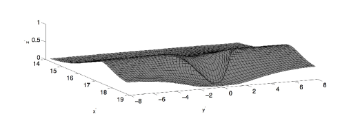
(b)

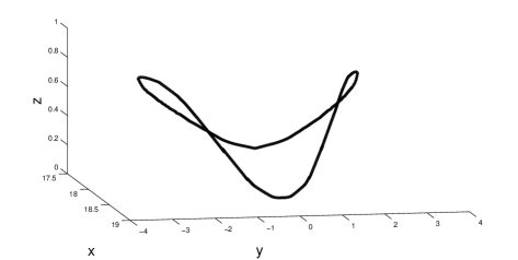
Figure 2: Numerical results at $t=1.378$ (based on GG ): (a) 3D wave profile; and (b) apparent contour

.

Some of the numerical results reported in GG are revisited below, and compared to the theoretical predictions of section II.2.

An idealized geometry was selected to simulate 3D breaking-waves on beaches, which is shown in figure 2 of ref.GG . The wave propagates towards the positive $x$ direction, where the water depth $z=-h_{0}$ is constant in the first part of the tank, then a sloping ridge starts at $x=5.22$ with a 1/15 slope in the middle cross-section and a transverse modulation of the form $sech^{2}(ky)$, with $k=0.25$ in the present case. (the non-dimensional variables $(x,y)$ being scaled with $h_{0}$ and time with $\sqrt{h_{0}/g}$). On such a bathymetric lens, that causes directional wave focusing, the wave first overturns on the axis, at $y=0$ and then breaking propagates laterally in both $\pm y$ directions. 3D wave profiles are shown in Figs. $5c,6c$, and $20$, of reference GG , for time values after overturning $t=1.036,1.252$ and $1.378$, respectively ($t=t^{\prime}-t^{\prime}_{B}$ in GG ’s notations).

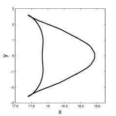
Figure 3: Numerical results (based on GG ): Projection of the apparent contour at time (left) $t=0.13$, (right) $t=1.378$

.

In Figure 2a, we reproduce the 3D wave profile at time $t=1.378$ just before the plunging jet reaches the underlying surface of the wave, and show in Figure 2b the apparent contour of the corresponding overhanging region. Figs. 3 displays apparent contours projected on the horizontal plane, both for this and an earlier time case, $t=0.13$. Both of these apparent contours are in good qualitative agreement with the theoretical predictions of equations (14)-(16), shown in Figure 1 for the same two values of $t$. Hence, even though the scaling laws were derived above for small values of ($t,u,x,y$) we observe that the ’generic equation’ derived in the previous subsection remains correct beyond this range of validity. Indeed the apparent contours for the latter time are very similar, see Figs. 2b and 3 (right), while the corresponding values of ($t,u,x,y$) become larger than unity.

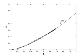
Figure 4: Numerical results (+) (based on GG ), compared to analytic prediction, equation (15): Growth of the overhanging region along the propagation direction $x$, as a function of $t=t^{\prime}-t^{\prime}_{B}$

.

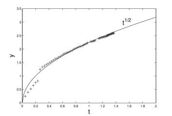
Figure 5: Numerical results (+) (based on GG ) compared to analytic prediction, equation (15): Growth of the overhanging region in the direction $y$ transverse to propagation as a function of $t=t^{\prime}-t^{\prime}_{B}$

.

Let us now test the scaling laws for the longitudinal and transverse expansions in time of the singularity (defined as $h(x,y,t)$ being multivalued in the overhanging region), representing the overturning wave. Thus, Figs. 4 and 5 show numerical results for the spatial expansion of the apparent contour along $x$ and $y$, respectively, as a function of the time increase from the beginning of the overturning. The two curves display a good fit with the power laws $t^{3/2}$ and $t^{1/2}$, respectively, as predicted by our analysis in section II.2. The discontinuity near time $t=0.23$ in Figure 5 is likely a numerical artifact due to the difficulty of accurately defining the apparent contour along the $y$ direction for small values of $t$. In summary the predictions of the ‘generic solution’(16), proposed above, are well confirmed by the simulations.

While these simple scaling laws have been confirmed, the asymmetry of the actual wave profile, due to the appearance of a plunging jet, cannot be described by the simple cubic term in the ($F,G$) expansion. In fact, the plunging jet can be viewed as a late evolution of a Rayleigh-Taylor instability, which occurs when a heavy liquid is placed over a lighter one. This phenomenon was recently studied in Clavin , where a finger in free fall was also observed in the late (and highly nonlinear) stage of the Rayleigh-Taylor instability. The 2D analysis of Clavin assumed a jet falling vertically (along $z$ in our notations) without horizontal velocity (along $x$). We will extend this work to estimate further properties of the overturning jet, by including an initial longitudinal velocity of the jet, $u_{0}$. Thus, in the overturning region, the tip of the jet follows a ballistic motion, with $z\sim{-\frac{1}{2}gt^{2}}$, and a quasi-constant horizontal velocity (see, e.g., Figure 12a of GG ). Scaling both time and position, as in Clavin , by factors $\sqrt{gk}$ and $k$ respectively (where $k$ is the wave number of the implemented sine perturbation of the interface) and changing their notations $y,v$ into $-z,w$ to avoid confusion with the above notations, the velocity field in the tip region is approximated by

$$\left\{\begin{array}[]{l}u\sim{u_{0}}\\ w\sim{-t}\sim{-\sqrt{2z}}\mathrm{.}\end{array}\right.$$ (17)

Now, the kinetic equation for the interface $\alpha(x,t)$ reads

$$\frac{\partial\alpha}{\partial t}+u_{0}\frac{\partial\alpha}{\partial x}=-\sqrt{2\alpha}\mathrm{.}$$ (18)

Defining $\alpha(x,t)=-t[t/2-\gamma(x,t)]$, we obtain after linearization

$$\frac{\partial\gamma}{\partial t}+u_{0}\frac{\partial\gamma}{\partial x}=0\mathrm{.}$$ (19)

which can be solved in the form, $\gamma(x,t)=\theta(x-u_{0}t)$. The curvature of the plunging tip is then defined as $\kappa=\frac{\partial^{2}\alpha}{\partial t^{2}}|_{x=u_{0}t}$. This yields the scaling relationship for the asymptotic evolution of the curvature

$$\kappa\sim|t|\theta_{0}^{"}\mathrm{.}$$ (20)

[Note that, without the horizontal velocity, one finds $\kappa\sim|t|^{3}\theta_{0}^{"}$.]

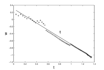
Figure 6: Numerical result (+) (based on GG ), compared to analytic prediction, second equation (17): Growth of the vertical velocity at the jet end, at $y=0$.

.

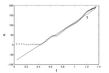
Figure 7: Numerical result (+) (based on GG ), compared to analytic prediction, equation (20): Growth of the curvature at the jet end, in the plane $y=0$.

.

We now posit that the predictions (17) and (20) of the asymptotic linear evolution of $w$ and $\kappa$ with time, are also valid in the 3D case. Indeed the first one simply reflects the ballistic motion, and the second one remains valid when the curvature of the wavefront along the crest is taken into account (this being time independent at leading order, see equation (16)). Figs. 6 and 7 confirm that the relationships (17) and (20) agree well with results of 3D simulations.

III Wave-breaking in shallow water

The analysis we presented before does not directly apply to actual waves, which are not physically described by the pressure-less fluid equations used so far. However, we will show below that, for surface waves propagating in shallow water, the equations governing wave motion reduce to the equations of a pressure-less fluid near the singularity.

Weakly nonlinear and dispersive inviscid long waves are well described by Boussinesq equations, when $A/h_{0}\sim(kh_{0})^{2}\ll 1$ Mei , with $A$ a characteristic wave amplitude, $k=2\pi/\lambda$, the wavenumber with $\lambda$ the wavelength, and $h_{0}$ the water depth from mean water level. More recently, extended Boussinesq models (BM) have been proposed that apply to strongly nonlinear waves, with $A/h_{0}={\cal O}(1)$, and have been shown to stay valid close to the breaking point Wei . In BMs, the fundamental quantities are the total fluid depth, $h(x,y,t)$ (i.e., from free surface to bottom) and the two Cartesian components of the horizontal fluid velocity, $u(x,y,t)$ and $v(x,y,t)$. The BM equations of motion express the conservation of mass and of horizontal momentum. Assuming fully nonlinear non-dispersive long waves, BM equations yield the ”nonlinear shallow water wave” equations Mei :

$$\left\{\begin{array}[]{l}\frac{\partial h}{\partial t}+\frac{\partial(uh)}{\partial x}+\frac{\partial(vh)}{\partial y}=0\\ \frac{\partial u}{\partial t}+u\frac{\partial u}{\partial x}+v\frac{\partial u}{\partial y}+g\frac{\partial h}{\partial x}=0\\ \frac{\partial v}{\partial t}+u\frac{\partial v}{\partial x}+v\frac{\partial v}{\partial y}+g\frac{\partial h}{\partial y}=0\mathrm{,}\end{array}\right.$$ (21)

where $g$ is the positive acceleration of gravity. Whenever all functions are independent of $y$, this set of equations admits nontrivial simple 1D wave solutions. We shall see that similar results also exist in 2D.

III.1 One-dimensional case

When the solution only depends on $x$, we can define $h=h_{0}+\tilde{h}(x,t)$ and, if we further assume that $h_{0}$ is much larger than the free surface perturbation $\tilde{h}(x,t)$, one may neglectMei terms of order $\tilde{h}(x,t)u$ with respect to terms of order $h_{0}u(x,t)$ in the BMs. This yields:

$$\left\{\begin{array}[]{l}\frac{\partial\tilde{h}}{\partial t}+u\frac{\partial\tilde{h}}{\partial x}+h_{0}\frac{\partial u}{\partial x}=0\\ \frac{\partial u}{\partial t}+u\frac{\partial u}{\partial x}+g\frac{\partial\tilde{h}}{\partial x}=0\mathrm{.}\end{array}\right.$$ (22)

Note that, although $\tilde{h}$ has been neglected with respect to $h_{0}$, one has kept the term $u\frac{\partial\tilde{h}}{\partial x}$ in the first equation, because a priori it is not smaller than any other term written explicitly in the second equation (22).

Let us now scale the lengths with $h_{0}$ and time with $\sqrt{h_{0}/g}$, that amounts to divide the velocity by the long wave celerity $C=\sqrt{gh_{0}}$. In terms of scaled variables, the equations for the new functions $\tilde{h}$ and $u$ thus become:

$$\left\{\begin{array}[]{l}\frac{\partial\tilde{h}}{\partial t}+u\frac{\partial\tilde{h}}{\partial x}+\frac{\partial u}{\partial x}=0\\ \frac{\partial u}{\partial t}+u\frac{\partial u}{\partial x}+\frac{\partial\tilde{h}}{\partial x}=0\mathrm{.}\end{array}\right.$$ (23)

If one assumes a simple wave solution of Equations 23, namely that $u=\tilde{h}$, the two equations become identical and yield the familiar (so-called) Burgers equation (1), when replacing $u$ (resp. $\tilde{h}$) by $(u+1)$ (resp.$(\tilde{h}+1)$). This shows that the singularity in these equations is the same one as found before. This is of course not a new result, because of the possibility of solving the full set of equations (21) by Riemann’s method with $v=0$ and no dependence on $y$.

III.2 Waves in two dimensions

Let us now use the full 2D equations (21) and thus define $h=h_{0}+\tilde{h}(x,y,t)$, with $\tilde{h}$ still being small, compared to $h_{0}$. Using the same scaling as above, the equations (21) for the mass and momentum conservation write in terms of scaled variables:

$$\left\{\begin{array}[]{l}\frac{\partial\tilde{h}}{\partial t}+\left(\frac{\partial u}{\partial x}+\frac{\partial v}{\partial y}\right)+u\frac{\partial\tilde{h}}{\partial x}+v\frac{\partial\tilde{h}}{\partial y}=0\\ \frac{\partial u}{\partial t}+u\frac{\partial u}{\partial x}+v\frac{\partial u}{\partial y}+\frac{\partial\tilde{h}}{\partial x}=0\\ \frac{\partial v}{\partial t}+u\frac{\partial v}{\partial x}+v\frac{\partial v}{\partial y}+\frac{\partial\tilde{h}}{\partial y}=0\mathrm{.}\end{array}\right.$$ (24)

To check whether these equations approach a pressure-less Bernouilli equation near the wave-breaking singularity, one assumes that the derivative $\frac{\partial v}{\partial y}$ is non-singular near this singularity, although $\frac{\partial u}{\partial x}$ diverges (which is true for simple waves, see below). Therefore one can neglect the former with respect to the latter. Hence, near the singularity, the first equation (24) may be replaced by

$$\frac{\partial\tilde{h}}{\partial t}+u\frac{\partial\tilde{h}}{\partial x}+v\frac{\partial\tilde{h}}{\partial y}+\frac{\partial u}{\partial x}=0\mathrm{.}$$ (25)

Now, if one assumes a simple wave solution, as in the 1D case, namely that $u=\tilde{h}$, Equation (25) becomes identical to the second equation (24). The first and second equations thus coalesce into $\frac{\partial u}{\partial t}+u\frac{\partial u}{\partial x}+v\frac{\partial u}{\partial y}+\frac{\partial u}{\partial x}=0\mathrm{.}$ Finally defining $\tilde{u}=u+1$, the set of equations (24) writes,

$$\left\{\begin{array}[]{l}\frac{\partial\tilde{u}}{\partial t}+\tilde{u}\frac{\partial\tilde{u}}{\partial x}+v\frac{\partial\tilde{u}}{\partial y}=0\\ \frac{\partial v}{\partial t}+\tilde{u}\frac{\partial v}{\partial x}+v\frac{\partial v}{\partial y}+(\frac{\partial\tilde{u}}{\partial y}-\frac{\partial v}{\partial x})=0\mathrm{,}\end{array}\right.$$ (26)

which is identical to the pressure-less fluid system (7), because the expression $(\frac{\partial\tilde{u}}{\partial y}-\frac{\partial v}{\partial x})$ vanishes for irrotational fluids.

This shows that, at least at leading order, wave-breaking scaling laws are identical for a pressure-less fluid and for the nonlinear shallow water wave equations.

This brings an interesting point: it seems that the widening of the wave-breaking domain in the $y$ direction, like the square root of time, is ’universal’ for non-linear non-dispersive waves. Other kinds of waves are known to break, like ocean waves on deep water (with, practically infinite depth). Does their spreading in the $y$ direction follow the same square root law ? The answer to this question depends in particular on how precisely one can identify the time for the onset of the breaking process. This deserves further investigations.

IV Discussion

IV.1 Regularisation

The regularization of the singularity appearing in solutions of the inviscid Burgers equation has been extensively studied. One such regularization scheme relies on an assumed balance of nonlinear and dispersive effects over a non-vanishing fluid depth. This yields the well-known Korteweg-de Vries (KdV) equation in 1D. This equation has been very thoroughly studied and can be shown to be a form of the standard Boussinesq equations when assuming wave propagation occurs in a forward direction only Mei . Hence, as for the standard weakly nonlinear and dispersive BM mentioned above, KdV equation requires that the two physically unrelated processes of nonlinearity and dispersion be of the same order. Hence, the range of applicability of this equation to water waves is quite narrow.

A second way to avoid the singularity consists in adding a small dissipative term to the inviscid Burgers equation (1) to make it ressemble the Navier-Stokes equation. This yields the so-called Burgers equation,

$$\frac{\partial u}{\partial t}+u\frac{\partial u}{\partial x}=\epsilon\frac{\partial^{2}u}{\partial x^{2}}\mathrm{,}$$ (27)

with the coefficient $\epsilon$ being small and positive. With a non-zero $\epsilon$ value, the solution of equation (27) is not multi-valued anymore (the equation is regularized) and one has to replace in the above analysis the multi-valued $U_{1}$ by a function with a jump at $\zeta=0$, which represents a shock wave for this model. By symmetry, the shock discontinuity is at $\zeta=0$. There, $U_{1}$ jumps from $+1$, for slightly negative values of $\zeta$, to $(-1)$, for slightly positive values of $\zeta$. In a small interval near $\zeta=0$, of width of order $(\epsilon t)^{1/2}$, the solution goes continuously from $+1$ to $(-1)$ across the shock front. Moreover, just at the time of the discontinuity, there is also a time interval where the added diffusion term is nowhere negligible. This time interval is such that the thickness of the self-similar region in $x$ is of the same order as the typical length scale associated with diffusion. The former decreases to zero as $t$ tends to zero, like $|t|^{2/3}$, and the latter like $(\epsilon t)^{1/2}$. The cross-over time is such that the two length scales are of the same order of magnitude, which happens for $t\sim\epsilon^{3}$. For time scales of this order or shorter, the self-similar solution is not valid anymore and another limit has to be taken. Real wave-breaking, however, cannot be described by this regularization, because it implies an overturning of the surface that is not represented by the viscous-like term on the right-hand side of equation (27).

IV.2 Geometrical meaning of the singularity or where is the true singularity?

Before proceeding further, it is worthwhile reconsidering the question of the singularity in light of a geometrical approach. This will yield a more precise definition of what we mean by wave-breaking. Let us get back to the ’generic’ solution (6) of the pressure-less fluid equation (1). In the simple wave case, this solution takes a simple geometrical meaning in which the two quantities $u$ (velocity component along the propagation direction) and $h$ (elevation of the fluid surface) are proportional to each other, up to irrelevant multiplicative constants. Then the 1D solution of,

$$0=h^{3}+x-ht\mathrm{}$$ (28)

can be seen as describing the occurrence of an apparent contour of a curve drawn on a plane, as it is continuously deformed, the deformation parameter being $t$. Such an apparent contour is defined (see section II) as the set of points where the tangent is parallel to the direction of observation, and the time origin $t=0$ is the instant where all points collapse into a single one. It is worthwhile noting that this definition depends upon the direction of observation. Indeed in 1D, at $t=0$, the local Cartesian equation of the curve is $h^{3}+x=0$, $h$ being the abscissa and $x$ the ordinate. As time changes, the curve is deformed and generically takes a non zero slope at the origin. The slope increases linearly with time, while the two extrema of the curve $x(h,t)$ move apart from each other, as $\Delta x\sim t^{3/2}$. Therefore the equation (28) describes the local shape of a line, when it acquires a contour at $t=0$. This contour is fundamentally linked to the direction of observation and would vanish if this direction were tilted in the direction parallel to the slope, at the inflection point. While it seems natural to choose the vertical axis as the observation direction in real life, we must note that the description of wave-breaking as the appearance of a contour is ambiguous.

To get round this difficulty let us note that wave-breaking could be defined either by the occurrence of overturning (i.e., an overhanging region on the surface), or by the impact and intersection of the plunging jet with the surface underneath. Casual observation indicates that the two phenomena are very strongly linked in the sense that overturning usually leads first to plunging and then to impact with the underlying surface. However things are not generally so simple, especially because the equations of motion are reversible (viscosity is negligible and thus neglected for this typically large Reynolds number flow). Hence, under time-reversal symmetry, a plunging jet would first retract onto itself and later return to a disappearing apparent contour.

Such a reversible event, namely the possibility of reversible overturning (i.e., the overhanging region spontaneously retracting instead of becoming a plunging jet), could possibly occur. This could happen, for instance, for a wave propagating over a decreasing depth, that would initiate overturning, then entering a region of rapidly increasing depth, which could make the overhanging region gradually disappear, provided its development has not proceeded too far in time. Another case could be that of a surface pressure (i.e, caused by wind) gradually increasing and ‘pushing’ against the nascent overturning region. Therefore an upward moving retracting jet is certainly among the solutions of the full dynamical problem and would lead quite naturally to define wave-breaking as the occurrence of self-penetration of the surface, a definition free of arbitrariness because, contrary to anything related to the apparent contour, it does not rely on an arbitrary choice of the direction of observation.

Seen from another perspective, wave-breaking now defined by the self-penetration of the surface by the plunging jet follows, but not always, from overturning of the surface. This raises also the very interesting issue of describing the post-penetration flow and surface intersection behavior (discussed below). Indeed regularization by capillary phenomena, viscosity, etc…may make this a well posed problem. Nevertheless we posit that the problem of impact between the plunging jet and the surface underneath it can be formulated in almost the same manner as the problem of propagation of nonlinear waves. This is discussed in the next subsection.

IV.3 Post collision dynamics

Classically the dynamics of nonlinear waves in the inviscid limit can be formulated as a system of two coupled first-order (in time) equations for the value of the velocity potential on the free surface and for the position of an arbitrary point on this surface. Let us briefly summarize the bases for this approach, in the usual case without collision of fluid interfaces. Knowing the value of the velocity potential on the free surface and, given the Neumann condition on the bottom, one can in principle solve the Dirichlet-like Boundary Integral Equation (BIE) problem for the velocity potential everywhere GG ; GGD . This yields in particular the velocity normal to the free surface that is used to advance this surface in time. The value of the velocity potential on the surface is then similarly advanced by time integrating the Bernoulli equation at every free surface point. The major advantage of this BIE method is that, in numerical studies, one can transform the problem of solving Laplace or Poisson’s equation over the entire domain into an integral equation on the surface, solvable by analytic function theory in 2D and by Green’s function method in both 2D and 3D Grilli ; GGD , short-cutting the computationally complex problem of drawing a smooth curve or a surface embedded in the geometrical space.

To summarize, one starts from the unsteady Bernoulli equation for the velocity potential $\Phi({\bf{r}},t)$:

$$\frac{\partial\Phi}{\partial t}+\frac{1}{2}\left(\nabla\Phi\right)^{2}+gz+\frac{p}{\rho}=0\mathrm{}$$ (29)

with $z$ the height, $\rho$ the mass density of the fluid and $p$ the pressure. This equation is expressed on the free surface of the fluid, located at $z=h({\bf{r}}_{H},t)$, where ${\bf{r}}_{H}$ is the set of horizontal coordinates. Note that if there is overturning, the function $h({\bf{r}}_{H},t)$ is not single-valued everywhere. Because the free surface is in contact with air, the atmospheric pressure is applied everywhere on the surface, whose variation can be neglected. Therefore, we can set $p=p_{a}=0$ at $z=h$ and equation (29) becomes:

$$\frac{\partial\Phi}{\partial t}=-\frac{1}{2}\left(\nabla\Phi\right)^{2}-gz|_{z=h({\bf{r}}_{H},t)}\mathrm{.}$$ (30)

The other conditions to be satisfied by $\Phi$ are mass conservation, which becomes Laplace’s equation:

$$\nabla^{2}\Phi=0\mathrm{,}$$ (31)

and the Neumann (no-flow) condition at the bottom (assumed for simplicity at $z=0$),

$$\frac{\partial\Phi}{\partial z}=0|_{z=0}\mathrm{.}$$ (32)

Given the value of $\Phi$ on the free surface and the Neumann condition at $z=0$, one can solve Laplace’s equation, once it is transformed into a linear BIE. Concretely this means that the normal derivative of $\Phi$ on the free surface can be found by solving an integral equation on the boundary, the remaining components of the gradient of $\Phi$, there, being known from the data. This allows us to compute the left-hand side of equation (30), from its right-hand side, and thus to advance the value of $\Phi$ on the free surface, in time. The evolution of the free surface elevation is given by the kinematic condition that it be a material surface, thus advected by the local fluid velocity ($w$ is the vertical fluid velocity):

$$\frac{\partial h}{\partial t}+\frac{\partial\Phi}{\partial x}\frac{\partial h}{\partial x}+\frac{\partial\Phi}{\partial y}\frac{\partial h}{\partial y}=w|_{z=h({\bf{r}}_{H},t)}\mathrm{.}$$ (33)

Equations (30) and (33), assuming that the velocity components are computed via the solution of Laplace’s equation (31) (by a BIE), define a closed problem for the coupled evolution of the velocity potential and the free surface. All of this, however, assumes that the free surface remains simply connected. The explicit form of the BIE problem is as follows. It uses the 3D free space Green’s function defined as Brebbia ,

$$G({\bf{x}},{\bf{x}}_{1})=\frac{1}{4\pi r}\mathrm{,}$$ (34)

with the normal derivative

$$\frac{\partial G({\bf{x}},{\bf{x}}_{1})}{\partial n}=-\frac{1}{4\pi}\frac{{\bf{r}}\cdot{\bf{n}}}{r^{3}}\mathrm{,}$$ (35)

and $r$ being the distance from point ${\bf{x}}=(x,y,z)$ to the reference point ${\bf{x}}_{1}=(x_{1},y_{1},z_{1})$, both being on the boundary, and $\bf{n}$ representing the outward normal unit vector to the boundary at point ${\bf{x}}$. Green’s second identity transforms Laplace’s equation into the BIE,

$$\alpha({\bf{x}}_{1})\Phi({\bf{x}}_{1})=\int_{\Gamma({\bf{x}})}\left[G({\bf{x}},{\bf{x}}_{1})\frac{\partial\Phi({\bf{x}})}{\partial n}-\Phi({\bf{x}})\frac{\partial G({\bf{x}},{\bf{x}}_{1})}{\partial n}\right]{\mathrm{d}}\Gamma\mathrm{,}$$ (36)

in which $\alpha({\bf{x}}_{1})=\frac{\theta_{1}}{4\pi}$, with $\theta_{1}$ the exterior solid angle made by the boundary at point ${\bf{x}}_{1}$ (i.e. $2\pi$ for a smooth boundary). Moreover ${\mathrm{d}}\Gamma$ is the element of area on the surface at position ${\bf{x}}$. The accurate numerical solution of BIE (36), with the bottom boundary condition (32), together with the time integration of Equations (30) and (33), allows simulating 3D overturning waves such as depicted in Figure 2a GGD ; GG , up to the time the plunging jet is about to impact the free surface underneath it.

IV.3.1 Generalisation of the Integral equation method

In the case of a plunging jet impacting the underlying surface, the domain becomes multi-connected and the above BIE cannot be used as such anymore. We discuss a way to extend this method to such cases. According to the Kelvin-Helmholtz theorem, for an inviscid fluid, no vorticity can be created outside of the domain boundary. In the present case, this applies to the boundary between the free falling overturning jet and the fluid underneath. Thus, assuming the jet does not immediately mixes with the impacted fluid (and this is in fact supported by some laboratory experiments for early times after impact) a vortex sheet can be specified on the surface separating the two fluids vortexsheet , to simulate the tangential velocity discontinuity that appears, such that the plunging jet may continue to exist as a region of potential flow beyond the time of intersection. Thus the jet has two parts, an upper one in contact with ambient air (where $p=0$) , and a lower part inside the underlying fluid, which is separated from the surrounding fluid by high pressure air (see Figure 8). Let us now derive a closed set of dynamical equations for quantities defined on surfaces, as in the previous case prior to intersection. For that purpose, we introduce three boundaries, labeled $B_{1}$, $B_{2}$ and $B_{3}$, respectively (see Figure 8). $B_{1}$ is the bottom at $z=0$, $B_{2}$ is the free surface between the air and the fluid, where the pressure is zero, and $B_{3}$ is the inner surface separating the fluid coming from the jet from the underlying fluid.

Figure 8: Scheme of the plunging jet

.

Because of the existence on $B_{3}$ of the vortex sheet, i.e., concentrated vorticity, one cannot take as dynamical function the value of the velocity potential there, since it jumps across this interface. Therefore we shall take $\frac{\partial\Phi({\bf{x}})}{\partial n}$ instead of $\Phi({\bf{x}})$, as dynamical variable on $B_{3}$ where the normal velocity and the normal acceleration have both to be continuous, to make the two sides of the boundary moving together. The BIE for $\Phi$ can be solved from the knowledge of $\frac{\partial\Phi}{\partial n}$ (Neumann condition) on $B_{1}$, $B_{2}$, and $\Phi$ on $B_{3}$ (Dirichlet condition). This yields the set of boundary conditions for solving the Laplace equation (31) inside the fluid. To advance in time and derive the dynamical equation for $\frac{\partial\Phi}{\partial n}$ on $B_{3}$, let us define $q=\frac{p}{\rho}+\frac{1}{2}\,\mid\nabla\Phi\mid^{2}$ that we shall call the dynamical pressure. By taking the Laplacian of the Bernoulli equation (29), and because $\Phi$ and $z$ are harmonic functions, one finds:

$$\Delta q=0\mathrm{.}$$ (37)

We are now ready to solve equation (37), using only two boundary conditions for $q$, $q=\frac{1}{2}\,\mid\nabla\Phi\mid^{2}$ on the free surface $B_{2}$ where $p=0$, plus the condition $\frac{\partial\left(q-\frac{1}{2}\,\mid\nabla\Phi\mid^{2}\right)}{\partial z}+g=0$ on the bottom $B_{1}$. Indeed the portion $B_{3}$ does not enter in the contour of the BIE for $q$, because both $q$ and $\frac{\partial q}{\partial n}$ are continuous on $B_{3}$ for the following reasons.

Defining the velocity as $\bf{\overrightarrow{u}}=-\bf{\overrightarrow{\nabla}}\Phi$, the Euler fluid equation can be written as,

$$\frac{\partial{\bf{\overrightarrow{u}}}}{\partial t}+\bf{\overrightarrow{\nabla}}q+g{\bf{e}}_{z}=0\mathrm{,}$$ (38)

where ${\bf{e}}_{z}$ is the unit vector in the vertical direction. The continuity of $q$ across $B_{3}$ follows from equation (38) since otherwise an infinite acceleration would take place. Moreover the continuity of $\frac{\partial q}{\partial n}$ is ensured because of the continuity of the normal acceleration across $B_{3}$. Therefore the Laplace equation (37) for $q$ can be solved by using the boundary conditions on $B_{1}$ and $B_{2}$ only.

This means that, like the problem of evolution of the free surface in the simply connected case, the post-collision dynamical equations (for $\Phi$ and $q$) can be reduced to linear integral equations posed on the boundaries ($B_{1,2,3}$ for $\Phi$, and $B_{1,2}$ for $q$).

Because of the merging of the plunging jet with the fluid underneath, vorticity is generated in a flow that is otherwise potential. This vorticity is roughly horizontal in the span-wise direction of the waves. If those waves are more or less parallel to each other (i.e., long crested) , this could be a coherent source of vorticity near the surface that would become on a large scale a shear layer driving the fluid opposite to the direction of the wave propagation. Another difficulty in this problem is the possible occurrence of regions of negative pressure where nucleation of bubbles should take place (actually of pressure less than the value of saturating pressure for the given temperature condition). We set aside this possibility, although it is obvious from observations that air bubbles are generated in white caps and even more so by plunging breakers.

IV.3.2 Hertz-fluid contact problem

A possible explanation for this generation of many bubbles lies in a simple scaling law for the Hertz-fluid contact problem. Let us assume that the plunging jet has a locally parabolic tip hitting the fluid underneath, for simplicity, assumed to be flat. Therefore we have a typical length scale, the radius of curvature of the parabolic tip $R$, and a velocity scale, the velocity $w$ of the falling jet when it hits the flat surface. Because Bernoulli equation has no intrinsic scale, every parameter, like for instance the typical value of the velocity in the collision region (defined a bit more accurately below), is like ${\bf{u}}(x,t)=w{\bf{u}}_{sc}(x/R,wt/R)$, where the vector field ${\bf{u}}_{sc}(x/R,wt/R)$ is dimensionless, universal, and defined by numerical functions only, $t=0$ being defined as the time of the first contact. One may try to find the behavior of the various quantities involved just after the collision by borrowing some of the ideas of the famous Hertz contact problem Hertz between solids. As in Hertz contact, one assumes that the perturbation comes from the flattening of the tip, wherever it would be inside the fluid underneath if this were possible. The tip would have penetrated by a length $wt$ inside this fluid, and so spread over a length of order $\lambda\sim(Rwt)^{1/2}$ along this surface. Because this brings a perturbation of order 1 to the boundary of the fluid inside the jet and because Laplace’s equation has no typical length scale (this argument is directly borrowed from Hertz’s contact problem, where Hertz used this property of the equations of elasticity), the region perturbed inside the jet is a volume of size $\lambda$ in all directions. The vertical momentum of the falling jet in this perturbed region is therefore of order

$$P_{z}\sim\rho w\lambda^{3}\mathrm{.}$$ (39)

The change with time of this momentum $\frac{dP_{z}}{dt}=p\lambda^{2}$ is due to the pressure $p$ near the boundary between the falling jet and the fluid underneath over an area $\lambda^{2}$. This yields an order of magnitude for the pressure in the collision domain

$$p\sim\rho w^{2}\left(\frac{R}{wt}\right)^{1/2}\mathrm{,}$$ (40)

when using the approximation $\frac{dP_{z}}{dt}\sim\frac{P_{z}}{t}$. The relation (40) shows that this pressure, felt across the boundary $B_{3}$, diverges at the instant of contact where it is regularized probably by capillary phenomena and/or compressibility effects in the fluid (in the compressible case, at short time, the divergence of pressure is replaced by a very large peak of pressure of order $\rho wc_{s}$, with $c_{s}$ the speed of sound in the fluid). This result could explain in part the formation of bubbles and foam in the real world.

V Final remarks

We presented a rather simplistic, but physically meaningful, approach to wave-breaking, yielding scaling laws that were shown to be in good agreement with numerical results for wave overturning in 3D, based on a higher-order solution of full dynamic equations. This work is an example of complementarity between advanced numerical and analytical methods, each providing validation and physical meaning to the other. Analytical methods also make it possible to generalize nonlinear properties observed in numerical results, to a whole class of equations and problems.

In particular, and on a more general point of view, it seems to us that many important concepts and ideas pertaining to nonlinear science remain to be exploited, in many areas where they can guide the intuition or better yield specific predictions that can then be compared to numerical results. In the specific application of nonlinear fluid mechanics presented here, we have encountered various more generic subproblems, all with a definitely very strong nonlinear flavor, like the singular behavior of solutions of partial differential equations, or what we referred to as the Hertz-fluid contact problem. In closing, this indicates that free boundary problems remain a rich and perhaps inexhaustible source of inspiration in the field of nonlinear science.

- (1) See for example the review paper by Dias F and Kharif C 1999 Nonlinear gravity and capillary-gravity waves Annu. Rev. Fluid Mech. 31 301-346.
- (2) Poisson S D 1808 Mémoire sur la théorie du son Journal de l’Ecole Polytechnique 14 éme cahier 7 319-392.
- (3) Zel’dovich Ya B 1970 Fragmentation of a homogeneous medium under the action of gravitation Astrofisica 6 319-335 [1973 Astrophysics 6 164-174].
- (4) Arnold V.I. 1984 Catastrophe theory (Springer Verlag, Berlin). See in particular Chapter 8 on Caustics and wavefronts.
- (5) Florin V A 1948 Izvestia Ak.Nauk SSSR Otd.Tekhn.Nauk 9 1389-1397.
- (6) P. Guyenne and S.T. Grilli 2006 Numerical study of three-dimensional overturning waves in shallow water. J. Fluid Mech. J. Fluid Mech. 547 361-388.
- (7) Pomeau Y, Jamin T, Le Bars M and Le Gal P 2008 Law of spreading of the crest of a breaking wave to be published in Proc. R. Soc. A 275 123-132; see also Pomeau Y, Le Bars M, Le Gal P, Jamin T, Le Berre M, Guyenne Ph, Grilli S and Audoly B 2008 Sur le déferlement des vagues , to be published in Compte-Rendus de la rencontre du Non-linéaire 2008, Paris (Non-lin aire Publications, Orsay France).
- (8) Dommermuth D G, Yue D K P, Lin W M, Rapp R J, Chan E S and Melville W K 1988 Deep-Water Plunging Breakers : a Comparison between Potential Theory and Experiments J. Fluid Mech. 189 423-442; Skinner D J 1996 A comparison of numerical predictions and experimental measurements of the internal kinematics of a deep-water plunging wave J. Fluid Mech. 315 51-64 (doi: 10.1017/S0022112096002327, Published online by Cambridge University Press 26 Apr 2006 ); Grilli S T, Svendsen I A and Subramania R 1997 Breaking Criterion and Characteristics for Solitary Waves on Slopes J. Waterway Port Coastal Ocean J. Waterway Port Coastal Ocean Engng. 123 102-112.
- (9) Duchemin L, Josserand C and Clavin P 2005 Asymptotic behavior of the Rayleigh-Taylor instability Phys. Rev. Lett. 94 1-4
- (10) Brebbia C A 1978 The Boundary Element Method for Engineers (Wiley, New York) .
- (11) Mei C C 1983 The Applied Dynamics of Ocean Surface Waves( World Scientific, Singapore).
- (12) Wei J, Kirby J T, Grilli S T, and Subramanya R A 1995 A Fully Nonlinear Boussinesq Model for Surface Waves. Part 1. Highly Nonlinear Unsteady Waves J. Fluid Mech. 294 71-92; Wei J, G and Kirby J T 1995 A time-dependent numerical code for extended Boussinesq equations J. Wtrwy, Port, Coast, and Oc. Engrg. 121 251-261; Kirby J T 2003 Boussinesq models and applications to nearshore wave propagation, surf zone processes and wave-induced currents 67 1-41 in Advances in Coastal Modeling ( V. C. Lakhan (ed) , Elsevier Oceanography Series ).
- (13) Grilli S T, Guyenne P, and Dias F 2001 A fully nonlinear model for three-dimensional overturning waves over arbitrary bottom Intl. J. Numer. Methods in Fluids, 35(7) 829-867.
- (14) Grilli S T and Hu Z 1998 A Higher-order Hypersingular Boundary Element Method for the Modeling of Vortex Sheet Dynamics Engng. Analysis Boundary Elemt. 21(2) 117-129.
- (15) Landau L D and Lifschitz E M 1970 Theory of Elasticity (Pergamon Press).