Multicast Capacity of Optical WDM Packet Ring for Hotspot Traffic

Abstract.

Packet-switching WDM ring networks with a hotspot transporting unicast, multicast, and broadcast traffic are important components of high-speed metropolitan area networks. For an arbitrary multicast fanout traffic model with uniform, hotspot destination, and hotspot source packet traffic, we analyze the maximum achievable long-run average packet throughput, which we refer to as multicast capacity, of bi-directional shortest-path routed WDM rings. We identify three segments that can experience the maximum utilization, and thus, limit the multicast capacity. We characterize the segment utilization probabilities through bounds and approximations, which we verify through simulations. We discover that shortest-path routing can lead to utilization probabilities above one half for moderate to large portions of hotspot source multi- and broadcast traffic, and consequently multicast capacities of less than two simultaneous packet transmissions. We outline a one-copy routing strategy that guarantees a multicast capacity of at least two simultaneous packet transmissions for arbitrary hotspot source traffic.

Keywords: Hotspot traffic, multicast, packet throughput, shortest path routing, spatial reuse, wavelength division multiplexing (WDM).

1. Introduction

Optical packet-switched ring wavelength division multiplexing (WDM) networks have emerged as a promising solution to alleviate the capacity shortage in the metropolitan area, which is commonly referred to as metro gap. Packet-switched ring networks, such as the Resilient Packet Ring (RPR) [1, 2, 3], overcome many of the shortcomings of circuit-switched ring networks, such as low provisioning flexibility for packet data traffic [4]. In addition, the use of multiple wavelength channels in WDM ring networks, see e.g., [5, 6, 7, 8, 9, 10, 11, 12, 13], overcomes a key limitation of RPR, which was originally designed for a single-wavelength channel in each ring direction. In optical packet-switched ring networks, the destination nodes typically remove (strip) the packets destined to them from the ring. This destination stripping allows the destination node as well as other nodes downstream to utilize the wavelength channel for their own transmissions. With this so-called spatial wavelength reuse, multiple simultaneous transmissions can take place on any given wavelength channel. Spatial wavelength reuse is maximized through shortest path routing, whereby the source node sends a packet in the ring direction that reaches the destination with the smallest hop distance, i.e., traversing the smallest number of intermediate network nodes.

Multicast traffic is widely expected to account for a large portion of the metro area traffic due to multi-party communication applications, such as tele-conferences [14], virtual private network interconnections, interactive distance learning, distributed games, and content distribution. These multi-party applications are expected to demand substantial bandwidths due to the trend to deliver the video component of multimedia content in the High-Definition Television (HDTV) format or in video formats with even higher resolutions, e.g., for digital cinema and tele-immersion applications. While there is at present scant quantitative information about the multicast traffic volume, there is ample anecdotal evidence of the emerging significance of this traffic type [15, 16]. As a result, multicasting has been identified as an important service in optical networks [17, 18] and has begun to attract significant attention in optical networking research as outlined in Section 1.1.

Metropolitan area networks consist typically of edge rings that interconnect several access networks (e.g., Ethernet Passive Optical Networks) and connect to a metro core ring [4]. The metro core ring interconnects several metro edge rings and connects to the wide area network. The node connecting a metro edge ring to the metro core ring is typically a traffic hotspot as it collects/distributes traffic destined to/originating from other metro edge rings or the wide area network. Similarly, the node connecting the metro core ring to the wide area network is typically a traffic hotspot. Examining the capacity of optical packet-switched ring networks for hotspot traffic is therefore very important.

In this paper we examine the multicast capacity (maximum achievable long run average multicast packet throughput) of bidirectional WDM optical ring networks with a single hotspot for a general fanout traffic model comprising unicast, multicast, and broadcast traffic. We consider an arbitrary traffic mix composed of uniform traffic, hotspot destination traffic (from regular nodes to the hotspot), and hotspot source traffic (from the hotspot to regular nodes). We study the widely considered node architecture that allows nodes to transmit on all wavelength channels, but to receive only on one channel. We initially examine shortest path routing by deriving bounds and approximations for the ring segment utilization probabilities due to uniform, hotspot destination, and hotspot source packet traffic. We prove that there are three ring segments (in a given ring direction) that govern the maximum segment utilization probability. For the clockwise direction in a network with nodes $1,2,\ldots,N$ and wavelengths $1,2,\ldots,\Lambda$ (with $N/\Lambda\geq 1$), whereby node 1 receives on wavelength 1, node 2 on wavelength 2, $\ldots$, node $\Lambda$ on wavelength $\Lambda$, node $\Lambda+1$ on wavelength 1, and so on, and with node $N$ denoting the index of the hotspot node, the three critical segments are identified as:

• the segment connecting the hotspot, node $N$, to node 1 on wavelength 1,

• the segment connecting node $\Lambda-1$ to node $\Lambda$ on wavelength $\Lambda$, and

• the segment connecting node $N-1$ to node $N$ on wavelength $\Lambda$.

The utilization on these three segments limits the maximum achievable multicast packet throughput. We observe from the derived utilization probability expressions that the utilizations of the first two identified segments exceed 1/2 (and approach 1) for large fractions of hotspot source multi- and broadcast traffic, whereas the utilization of the third identified segment is always less than or equal to 1/2. Thus, shortest path routing achieves a long run average multicast throughput of less than two simultaneous packet transmissions (and approaching one simultaneous packet transmission) for large portions of hotspot source multi- and broadcast traffic.

We specify one-copy routing which sends only one packet copy for hotspot source traffic, while uniform and hotspot destination packet traffic is still served using shortest path routing. One-copy routing ensures a capacity of at least two simultaneous packet transmissions for arbitrary hotspot source traffic, and at least approximately two simultaneous packet transmissions for arbitrary overall traffic. We verify the accuracy of our bounds and approximations for the segment utilization probabilities, which are exact in the limit $N/\Lambda\rightarrow\infty$, through comparisons with utilization probabilities obtained from discrete event simulations. We also quantify the gains in maximum achievable multicast throughput achieved by the one-copy routing strategy over shortest path routing through simulations.

This paper is structured as follows. In the following subsection, we review related work. In Section 2, we introduce the detailed network and traffic models and formally define the multicast capacity. In Section 3, we establish fundamental properties of the ring segment utilization in WDM packet rings with shortest path routing. In Section 4, we derive bounds and approximations for the ring segment utilization due to uniform, hotspot destination, and hotspot source packet traffic on the wavelengths that the hotspot is not receiving on, i.e., wavelengths $1,2,\ldots,\Lambda-1$ in the model outlined above. In Section 5, we derive similar utilization probability bounds and approximations for wavelength $\Lambda$ that the hotspot receives on. In Section 6, we prove that the three specific segments identified above govern the maximum segment utilization and multicast capacity in the network, and discuss implications for packet routing. In Section 7, we present numerical results obtained with the derived utilization bounds and approximations and compare with verifying simulations. We conclude in Section 8.

1.1. Related Work

There has been increasing research interest in recent years for the wide range of aspects of multicast in general mesh circuit-switched WDM networks, including lightpath design, see for instance [19], traffic grooming, see e.g., [20], routing and wavelength assignment, see e.g., [21, 22, 23], and connection carrying capacity [24]. Similarly, multicasting in packet-switched single-hop star WDM networks has been intensely investigated, see for instance [25, 26, 27, 28]. In contrast to these studies, we focus on packet-switched WDM ring networks in this paper.

Multicasting in circuit-switched WDM rings, which are fundamentally different from the packet-switched networks considered in this paper, has been extensively examined in the literature. The scheduling of connections and cost-effective design of bidirectional WDM rings was addressed, for instance in [29]. Cost-effective traffic grooming approaches in WDM rings have been studied for instance in [30, 31]. The routing and wavelength assignment in reconfigurable bidirectional WDM rings with wavelength converters was examined in [32]. The wavelength assignment for multicasting in circuit-switched WDM ring networks has been studied in [33, 34, 35, 36, 37, 38]. For unicast traffic, the throughputs achieved by different circuit-switched and packet-switched optical ring network architectures are compared in [39].

Optical packet-switched WDM ring networks have been experimentally demonstrated, see for instance [13, 40], and studied for unicast traffic, see for instance [5, 41, 6, 7, 8, 9, 10, 11, 12, 13]. Multicasting in packet-switched WDM ring networks has received increasing interest in recent years [42, 10]. The photonics level issues involved in multicasting over ring WDM networks are explored in [43], while a node architecture suitable for multicasting is studied in [44]. The general network architecture and MAC protocol issues arising from multicasting in packet-switched WDM ring networks are addressed in [40, 45]. The fairness issues arising when transmitting a mix of unicast and multicast traffic in a ring WDM network are examined in [46]. The multicast capacity of packet-switched WDM ring networks has been examined for uniform packet traffic in [47, 48, 49, 50]. In contrast, we consider non-uniform traffic with a hotspot node, as it commonly arises in metro edge rings [51].

Studies of non-uniform traffic in optical networks have generally focused on issues arising in circuit-switched optical networks, see for instance [52, 53, 54, 55, 56, 57, 58]. A comparison of circuit-switching to optical burst switching network technologies, including a brief comparison for non-uniform traffic, was conducted in [59]. The throughput characteristics of a mesh network interconnecting routers on an optical ring through fiber shortcuts for non-uniform unicast traffic were examined in [60]. The study [61] considered the throughput characteristics of a ring network with uniform unicast traffic, where the nodes may adjust their send probabilities in a non-uniform manner. The multicast capacity of a single-wavelength packet-switched ring with non-uniform traffic was examined in [62]. In contrast to these works, we consider non-uniform traffic with an arbitrary fanout, which accommodates a wide range of unicast, multicast, and broadcast traffic mixes, in a WDM ring network.

2. System Model and Notations

We let $N$ denote the number of network nodes, which we index sequentially by $i,\,\,i=1,\ldots,N$, in the clockwise direction and let $\mathcal{M}:=\left\{1,\ldots,N\right\}$ denote the set of network nodes. For convenience, we label the nodes modulo $N$, e.g., node $N$ is also denoted by $0$ or $-N$. We consider the family of node structures where each node can transmit on any wavelength using either one or multiple tunable transmitters $\left(TTs\right)$ or an array of $\Lambda$ fixed-tuned transmitters $\left(FT^{\Lambda}\right)$, and receive on one wavelength using a single fixed-tuned receiver $\left(FR\right)$.

For $N=\Lambda$, each node has its own home channel for reception. For $N>\Lambda$, each wavelength is shared by $\eta:=N/\Lambda$ nodes, which we assume to be an integer. For $1\leq i\leq N$, we let $\overset{\curvearrowright}{u}_{i}$ denote the clockwise oriented ring segment connecting node $i-1$ to node $i$. Analogously, we let $\overset{\curvearrowleft}{u}_{i}$ denote the counter clockwise oriented ring segment connecting node $i$ to node $i-1$. Each ring deploys the same set of wavelength channels $\left\{1,\ldots,\Lambda\right\}$, one set on the clockwise ring and another set on the counterclockwise ring. The nodes $n=\lambda+k\Lambda$ with $k\in\left\{0,1,\ldots,\eta-1\right\}$ share the drop wavelength $\lambda$. We refer to the incoming edges of these nodes, i.e., the edges $\overset{\curvearrowright}{u}_{\lambda+k\Lambda}$ and $\overset{\curvearrowleft}{u}_{\lambda+1+k\Lambda}$, as critical edges on $\lambda$.

Figure 2.1. Illustration of the clockwise wavelength channels of a WDM ring network with $N=16$ nodes and $\Lambda=4$ wavelength channels.

For multicast traffic, the sending node generates a copy of the multicast packet for each wavelength that is drop wavelength for at least one destination node. Denote by $S$ the node that is the sender. We introduce the random set of destinations (fanout set) $\mathcal{F}\subset(\{1,2,\ldots,N\}\setminus\{S\}).$ Moreover, we define the set of active nodes $\mathcal{A}$ as the union of the sender and all destinations, i.e., $\mathcal{A}:=\mathcal{F}\cup\left\{S\right\}$.

We consider a traffic model combining a portion $\alpha$ of uniform traffic, a portion $\beta$ of hotspot destination traffic, and a portion $\gamma$ of hotspot source traffic with $\alpha,\beta,\gamma\geq 0$ and $\alpha+\beta+\gamma=1$:

Uniform traffic:

A given generated packet is a uniform traffic packet with probability $\alpha$. For such a packet, the sending node is chosen uniformly at random amongst all network nodes $\{1,2,\ldots,N\}$. Once the sender $S$ is chosen, the number of receivers (fanout) $l\in\{1,2,\ldots,N-1\}$ is chosen at random according to a discrete probability distribution $(\mu_{l})_{l=1}^{N-1}$. Once the fanout $l$ is chosen, the random set of destinations (fanout set) $\mathcal{F}\subset(\{1,2,\ldots,N\}\setminus\{S\})$ is chosen uniformly at random amongst all subsets of $\{1,2,\ldots,N\}\setminus\{S\}$ having cardinality $l$. We denote by $P_{\alpha}$ the probability measure associated with uniform traffic.

Hotspot destination traffic:

A given packet is a hotspot destination traffic packet with probability $\beta$. For a hotspot destination traffic packet, node $N$ is always a destination. The sending node is chosen uniformly at random amongst the other nodes $\{1,2,\ldots,N-1\}$. Once the sender $S$ is chosen, the fanout $l\in\{1,2,\ldots,N-1\}$ is chosen at random according to a discrete probability distribution $(\nu_{l})_{l=1}^{N-1}$. Once the fanout $l$ is chosen, a random fanout subset $\mathcal{F}^{\prime}\subset(\{1,2,\ldots,N-1\}\setminus\{S\})$ is chosen uniformly at random amongst all subsets of $\{1,2,\ldots,N-1\}\setminus\{S\}$ having cardinality $(l-1)$, and the fanout set is $\mathcal{F}=\mathcal{F}^{\prime}\cup\{N\}$. We denote by $Q_{\beta}$ the probability measure associated with hotspot destination traffic.

Hotspot source traffic:

A given packet is a hotspot source traffic packet with probability $\gamma$. For such a packet, the sending node is chosen to be node $N$. The fanout $1\leq l\leq(N-1)$ is chosen at random according to a discrete prob. distribution $(\kappa_{l})_{l=1}^{N-1}$. Once the fanout $l$ is chosen, a random fanout set $\mathcal{F}\subset\{1,2,\ldots,N-1\}$ is chosen uniformly at random amongst all subsets of $\{1,2,\ldots,N-1\}$ having cardinality $l$. We denote by $Q_{\gamma}$ the probability measures associated with hotspot source traffic.

While our analysis assumes that the traffic type, the source node, the fanout, and the fanout set are drawn independently at random, this independence assumption is not critical for the analysis. Our results hold also for traffic patterns with correlations, as long as the long run average segment utilizations are equivalent to the utilizations with the independence assumption. For instance, our results hold for a correlated traffic model where a given source node transmits with a probability $p<1$ to exactly the same set of destinations as the previous packet sent by the node, and with probability $1-p$ to an independently randomly drawn number and set of destination nodes.

We denote by $P_{\alpha}^{l}$ the probability measure $P_{\alpha}$ conditioned upon $\left|\mathcal{F}\right|=l$, and define $Q_{\beta}^{l}$ and $Q_{\gamma}^{l}$ analogously. We denote the set of nodes with drop wavelength $\lambda$ by

(2.1) $$\mathcal{M}_{\lambda}:=\left\{\lambda+k\Lambda\,|\,k\in\left\{0,\ldots,\eta-1\right\}\right\}.$$

The set of all destinations with drop wavelength $\lambda$ is then

(2.2) $$\mathcal{F}_{\lambda}:=\mathcal{F}\cap\mathcal{M}_{\lambda}.$$

Moreover, we use the following notation: For $\ell\in\left\{1,\ldots,N-1\right\}$ we denote the probability of $\ell$ destinations on wavelength $\lambda$ by $\mu_{\lambda,\ell}$, $\nu_{\lambda,\ell}$, and $\kappa_{\lambda,\ell}$ for uniform, hotspot destination, and hotspot source traffic, respectively. Since the fanout set is chosen uniformly at random among all subsets of $\{1,2,\ldots,N\}\setminus\{S\}$ having cardinality $l$, these usage-probabilities can be expressed by $\mu_{l}$, $\nu_{l}$, and $\kappa_{l}$. Depending on whether the sender is on the drop-wavelength or not, we obtain slightly different expressions. As will become evident shortly, it suffices to focus on the case where the sender is on the considered drop wavelength $\lambda$, i.e., $S\in\mathcal{M}_{\lambda}$, since the relevant probabilities are estimated through comparisons with transformations (enlarged, reduced or right/left-shifted ring introduced in Appendix A) that put the sender in $\mathcal{M}_{\lambda}$.

Through elementary combinatorial considerations we obtain the following probability distributions: For uniform traffic, the probability for having $\ell\in\left\{0,\ldots,l\wedge\eta\right\}$ destinations on wavelength $\lambda$ is

(2.3) $$\mu_{\lambda,\ell}:=\sum_{l=\max(1,\ell)}^{N-1}\frac{{{\eta\choose\ell}}{{N-\eta\choose l-\ell}}}{{{N\choose l}}}\mu_{l}.$$

For hotspot destination traffic, we obtain for wavelengths $\lambda\neq\Lambda$ and $\ell\in\left\{0,\ldots,(l-1)\wedge\eta\right\}$

(2.4) $$\nu_{\lambda,\ell}:=\sum_{l=\max(1,\ell)}^{N-1}\frac{{{\eta\choose\ell}}{{N-\eta-1\choose l-\ell-1}}}{{{N-1\choose l-1}}}\nu_{l},$$

as well as for wavelength $\Lambda$ homing the hotspot and $\ell\in\left\{1,\ldots,l\wedge\eta\right\}$

(2.5) $$\nu_{\Lambda,\ell}:=\sum_{l=1}^{N-1}\frac{{{\eta-1\choose\ell-1}}{{N-\eta\choose l-\ell}}}{{{N-1\choose l-1}}}\nu_{l}.$$

Finally, for hotspot source traffic, we obtain for $\lambda\neq\Lambda$ and $\ell\in\left\{0,\ldots,l\wedge\eta\right\}$

(2.6) $$\kappa_{\lambda,\ell}:=\sum_{l=\max(1,\ell)}^{N-1}\frac{{{\eta\choose\ell}}{{N-1-\eta\choose l-\ell}}}{{{N-1\choose l}}}\kappa_{l}$$

and for $\lambda=\Lambda$ and $\ell\in\left\{0,\ldots,l\wedge(\eta-1)\right\}$

(2.7) $$\kappa_{\Lambda,\ell}:=\sum_{l=\max(1,\ell)}^{N-1}\frac{{{\eta-1\choose\ell}}{{N-\eta\choose l-\ell}}}{{{N-1\choose l}}}\kappa_{l}.$$

For a given wavelength $\lambda$, we denote by $p_{\alpha,\lambda}^{\ell}$ the probability measure $P_{\alpha}$ conditioned upon $\left|\mathcal{F}_{\lambda}\right|=\ell$, and define $q_{\beta,\lambda}^{\ell}$ and $q_{\gamma,\lambda}^{\ell}$ analogously.

Remark 2.1.

Whenever it is clear which wavelength $\lambda$ is considered we omit the subscript $\lambda$ and write $p_{\alpha}^{\ell},\,q_{\beta}^{\ell}$, or $q_{\gamma}^{\ell}$.

We introduce the set of active nodes $\mathcal{A}_{\lambda}$ on a given drop wavelength $\lambda$ as

(2.8) $$\mathcal{A}_{\lambda}:=\mathcal{F}_{\lambda}\cup\left\{S\right\}.$$

We order the nodes in this set in increasing order of their node indices, i.e.,

(2.9) $$\mathcal{A}_{\lambda}=\{X_{\lambda,1},X_{\lambda,2},\ldots,X_{\lambda,\ell+1}\},\quad 1\leq X_{\lambda,1}<X_{\lambda,2}<\ldots<X_{\lambda,\ell+1}\leq N,$$

and consider the “gaps”

(2.10) $$X_{\lambda,1}+(N-X_{\lambda,\ell+1}),\,(X_{\lambda,2}-X_{\lambda,1}),\ldots,\,(X_{\lambda,\ell+1}-X_{\lambda,\ell}),$$

between successive nodes in the set $\mathcal{A}_{\lambda}.$ We have denoted here again by $\ell\equiv\ell_{\lambda}$ the random number of destinations with drop wavelength $\lambda$.

For shortest path routing, i.e., to maximize spatial wavelength reuse, we determine the largest of these gaps. Since there may be a tie among the largest gaps (in which case one of the largest gaps is chosen uniformly at random), we denote the selected largest gap as “$CLG_{\lambda}$”¨ (for “Chosen Largest Gap”). Suppose the $CLG_{\lambda}$ is between nodes $X_{\lambda,i-1}$ and $X_{\lambda,i}$. With shortest path routing, the packet is then sent from the sender $S$ to node $X_{\lambda,i-1}$, and from the sender $S$ to node $X_{\lambda,i}$ in the opposite direction. Thus, the largest gap is not traversed by the packet transmission.

Note that by symmetry, $\mathbb{P}\{\overset{\curvearrowright}{u}_{1}\text{ is used}\}=\mathbb{P}\{\overset{\curvearrowleft}{u}_{N}\text{ is used}\}$, and $\mathbb{P}\{\overset{\curvearrowright}{u}_{N}\text{ is used}\}=\mathbb{P}\{\overset{\curvearrowleft}{u}_{1}\text{ is used}\}$. More generally, for reasons of symmetry, it suffices to compute the utilization probabilities for the clockwise oriented edges. For $n\in\left\{1,\ldots,N\right\}$, we abbreviate

(2.11) $$\overset{\curvearrowright}{n}_{\lambda}:=\overset{\curvearrowright}{u_{n}}\textrm{ is used on wavelength }\lambda.$$

It will be convenient to call node $N$ also node $0$. We let $\mathcal{G}_{\lambda},\ \mathcal{G}_{\lambda}=0,\ldots,N-1$, be a random variable denoting the first node bordering the chosen largest gap on wavelength $\lambda$, when this gap is considered clockwise.

The utilization probability for the clockwise segment $n$ on wavelength $\lambda$ is given by

(2.12) $$\mathbb{P}\left(\overset{\curvearrowright}{n}_{\lambda}\right)=\sum_{\ell=0}^{\eta}\left(\alpha\cdot p_{\alpha}^{\ell}\left(\overset{\curvearrowright}{n}_{\lambda}\right)\cdot\mu_{\lambda,\ell}+\beta\cdot q_{\beta}^{\ell}\left(\overset{\curvearrowright}{n}_{\lambda}\right)\cdot\nu_{\lambda,\ell}+\gamma\cdot q_{\gamma}^{\ell}\left(\overset{\curvearrowright}{n}_{\lambda}\right)\cdot\kappa_{\lambda,\ell}\right).$$

Our primary performance metric is the maximum packet throughout (stability limit). More specifically, we define the (effective) multicast capacity $C_{M}$ as the maximum number of packets (with a given traffic pattern) that can be sent simultaneously in the long run, and note that $C_{M}$ is given as the reciprocal of the largest ring segment utilization probability, i.e.,

(2.13) $$C_{M} := \frac{1}{\max_{n\in\left\{1,\ldots,N\right\}}\max_{\lambda\in\left\{1,\ldots,\Lambda\right\}}\mathbb{P}\left(\overset{\curvearrowright}{n}_{\lambda}\right)}.$$

3. General Properties of Segment Utilization

First, we prove a general recursion formula for shortest path routing.

Proposition 3.1.

Let $\lambda\in\left\{1,\ldots,\Lambda\right\}$ be a fixed wavelength. For all nodes $n\in\left\{0,\ldots,N-1\right\}$,

(3.1) $$\mathbb{P}\left(\overset{\curvearrowright}{(n+1)}_{\lambda}\right) = \mathbb{P}\left(\overset{\curvearrowright}{n}_{\lambda}\right)+\mathbb{P}\left(S=n\right)-\mathbb{P}\left(\mathcal{G}_{\lambda}=n\right).$$

Proof.

There are two complementary events leading to $\overset{\curvearrowright}{(n+1)}_{\lambda}$: (A) the packet traverses (on wavelength $\lambda$) both the clockwise segment $\overset{\curvearrowright}{u}_{n+1}$ and the preceding clockwise segment $\overset{\curvearrowright}{u}_{n}$, i.e., the sender is a node $S\neq n$, and (B) node $n$ is the sender ($S=n$) and transmits the packet in the clockwise direction, so that it traverses segment $\overset{\curvearrowright}{u}_{n+1}$ following node $n$ (in the clockwise direction). Formally,

(3.2) $$\mathbb{P}\left(\overset{\curvearrowright}{(n+1)}_{\lambda}\right) = \mathbb{P}\left(\overset{\curvearrowright}{n}_{\lambda}\text{ and }\overset{\curvearrowright}{(n+1)}_{\lambda}\right)+\mathbb{P}\left(S=n\textrm{ and }\overset{\curvearrowright}{(n+1)}_{\lambda}\right).$$

Next, note that the event that the clockwise segment $\overset{\curvearrowright}{u}_{n}$ is traversed can be decomposed into two complementary events, namely (a) segments $\overset{\curvearrowright}{u}_{n}$ and $\overset{\curvearrowright}{u}_{n+1}$ are traversed, and (b) segment $\overset{\curvearrowright}{u}_{n}$ is traversed, but not segment $\overset{\curvearrowright}{u}_{n+1}$, i.e.,

(3.3) $$\mathbb{P}\left(\overset{\curvearrowright}{n}_{\lambda}\right) = \mathbb{P}\left(\overset{\curvearrowright}{n}_{\lambda}\text{ and }\overset{\curvearrowright}{(n+1)}_{\lambda}\right)+\mathbb{P}\left(\overset{\curvearrowright}{n}_{\lambda}\textrm{ and not }\overset{\curvearrowright}{(n+1)}_{\lambda}\right).$$

Similarly, we can decompose the event of node $n$ being the sender as

(3.4) $$\mathbb{P}\left(S=n\right)=\mathbb{P}\left(S=n\textrm{ and }\overset{\curvearrowright}{(n+1)}_{\lambda}\right)+\mathbb{P}\left(S=n\textrm{ and not }\overset{\curvearrowright}{(n+1)}_{\lambda}\right).$$

Hence, we can express $\mathbb{P}\left(\overset{\curvearrowright}{(n+1)}_{\lambda}\right)$ as

(3.5) $$\mathbb{P}\left(\overset{\curvearrowright}{(n+1)}_{\lambda}\right) = \mathbb{P}\left(\overset{\curvearrowright}{n}_{\lambda}\right)-\mathbb{P}\left(\overset{\curvearrowright}{n}_{\lambda}\textrm{ and not }\overset{\curvearrowright}{(n+1)}_{\lambda}\right)$$

$$+\mathbb{P}\left(S=n\right)-\mathbb{P}\left(S=n\textrm{ and not }\overset{\curvearrowright}{(n+1)}_{\lambda}\right).$$

Now, note that there are two complementary events that result in the CLG to start at node $n$, such that clockwise segment $n+1$ is inside the CLG: $(i)$ node $n$ is the last destination node reached by the clockwise transmission, i.e., segment $n$ is used, but segment $n+1$ is not used, and $(ii)$ node $n$ is the sender and transmits only a packet copy in the counter clockwise direction. Hence,

(3.6) $$\mathbb{P}\left(\mathcal{G}_{\lambda}=n\right) = \mathbb{P}\left(\overset{\curvearrowright}{n}_{\lambda}\textrm{ and not }\overset{\curvearrowright}{(n+1)}_{\lambda}\right)+\mathbb{P}\left(S=n\textrm{ and not }\overset{\curvearrowright}{(n+1)}_{\lambda}\right).$$

Therefore, we obtain the general recursion

(3.7) $$\mathbb{P}\left(\overset{\curvearrowright}{(n+1)}_{\lambda}\right)=\mathbb{P}\left(\overset{\curvearrowright}{n}_{\lambda}\right)+\mathbb{P}\left(S=n\right)-\mathbb{P}\left(\mathcal{G}_{\lambda}=n\right).$$

∎

We introduce the left (counter clockwise) shift and the right (clockwise) shift of node $n$ to be $\left\lfloor n\right\rfloor_{\lambda}$ and $\left\lceil n\right\rceil_{\lambda}$ given by

(3.8) $$\left\lfloor n\right\rfloor_{\lambda}:=\left\lfloor\frac{n-\lambda}{\Lambda}\right\rfloor\Lambda+\lambda\textrm{ and }\left\lceil n\right\rceil_{\lambda}:=\left\lceil\frac{n-\lambda}{\Lambda}\right\rceil\Lambda+\lambda.$$

The counter clockwise shift maps a node $n$ not homed on $\lambda$ onto the nearest node in the counter clockwise direction that is homed on $\lambda$. Similarly, the clockwise shift maps a node $n$ not homed on $\lambda$ onto the closest node in the clockwise direction that is homed on $\lambda$.

For the traffic on wavelength $\lambda$, we obtain by repeated application of Proposition 3.1

(3.9) $$\mathbb{P}\left(\overset{\curvearrowright}{\left(\left\lceil n\right\rceil_{\lambda}\right)}_{\lambda}\right) = \mathbb{P}\left(\overset{\curvearrowright}{n}_{\lambda}\right)+\sum_{i=n}^{\lceil n\rceil_{\lambda}-1}\mathbb{P}\left(S=i\right)-\sum_{i=n}^{\lceil n\rceil_{\lambda}-1}\mathbb{P}\left(\mathcal{G}_{\lambda}=i\right)$$

(3.10) $$= \mathbb{P}\left(\overset{\curvearrowright}{n}_{\lambda}\right)+\mathbb{P}\left(S\in\left\{n,\ldots,\lceil n\rceil_{\lambda}-1\right\}\right)-\mathbb{P}\left(\mathcal{G}_{\lambda}\in\left\{n,\ldots,\lceil n\rceil_{\lambda}-1\right\}\right).$$

Note that the CLG on $\lambda$ can only start $(i)$ at the source node, irrespective of whether it is on $\lambda$, or $(ii)$ at a destination node on $\lambda$. Consider a given node $n$ that is not on $\lambda$, then the nodes in $\{n,\ n+1,\ldots,\lceil n\rceil_{\lambda}-1\}$ are not on $\lambda$. (If node $n$ is on $\lambda$, i.e., $n=\lceil n\rceil_{\lambda}$, then trivially the set $\{n,\ n+1,\ldots,\lceil n\rceil_{\lambda}-1\}$ is empty and $\mathbb{P}\left(\overset{\curvearrowright}{\left(\left\lceil n\right\rceil_{\lambda}\right)}_{\lambda}\right)=\mathbb{P}\left(\overset{\curvearrowright}{n}_{\lambda}\right)$.) Hence, the CLG on $\lambda$ can only start at a node in $\{n,\ n+1,\ldots,\lceil n\rceil_{\lambda}-1\}$ if that node is the source node, i.e.,

(3.11) $$\mathbb{P}\left(\mathcal{G}_{\lambda}\in\left\{n,\ldots,\lceil n\rceil_{\lambda}-1\right\}\right)=\mathbb{P}\left(\mathcal{G}_{\lambda}=S\in\left\{n,\ldots,\lceil n\rceil_{\lambda}-1\right\}\right).$$

Next, note that the event that a node in $\{n,\ n+1,\ldots,\lceil n\rceil_{\lambda}-1\}$ is the source node can be decomposed into the two complementary events $(i)$ a node in $\{n,\ n+1,\ldots,\lceil n\rceil_{\lambda}-1\}$ is the source node and the CLG on $\lambda$ starts at that node, and $(ii)$ a node in $\{n,\ n+1,\ldots,\lceil n\rceil_{\lambda}-1\}$ is the source node and the CLG does not start at that node. Hence,

(3.12) $$\mathbb{P}\left(S\in\left\{n,\ldots,\lceil n\rceil_{\lambda}-1\right\}\right)=\mathbb{P}\left(\mathcal{G}_{\lambda}=S\in\left\{n,\ldots,\lceil n\rceil_{\lambda}-1\right\}\right)+\mathbb{P}\left(S\in\left\{n,\ldots,m-1\right\},\mathcal{G}_{\lambda}\neq S\right).$$

Inserting (3.11) and (3.12) in (3.10) we obtain

(3.13) $$\mathbb{P}\left(\overset{\curvearrowright}{\left(\left\lceil n\right\rceil_{\lambda}\right)}_{\lambda}\right)=\mathbb{P}\left(\overset{\curvearrowright}{n}_{\lambda}\right)+\mathbb{P}\left(S\in\left\{n,\ldots,m-1\right\},\mathcal{G}_{\lambda}\neq S\right)$$

which directly leads to

Corollary 3.2.

The usage of non-critical segments is smaller than the usage of critical segments, more precisely for $n\in\left\{0,\ldots,N-1\right\}$:

(3.14) $$\mathbb{P}\left(\overset{\curvearrowright}{n}_{\lambda}\right) = \mathbb{P}\left(\overset{\curvearrowright}{\left(\left\lceil n\right\rceil_{\lambda}\right)}_{\lambda}\right)-\mathbb{P}\left(S\in\left\{n,\ldots,\left\lceil n\right\rceil_{\lambda}-1\right\},\mathcal{G}_{\lambda}\neq S\right).$$

To compare the expected length of the largest gap on a wavelength in the WDM ring with the expected length of the largest gap in the single wavelength ring, we introduce the enlarged and reduced ring in Appendix A. In brief, in the enlarged ring, an extra node is added on the considered wavelength between the $\lambda$-neighbors of the source node. This enlargement results in $(a)$ a set of $\eta+1$ nodes homed on the considered wavelength, and $(b)$ an enlarged set of active nodes $\mathcal{A}_{\lambda}^{+}$ containing the original destination nodes plus the added extra node (which in a sense represents the source node on the considered wavelength) for a total of $\ell+1$ active nodes. The expected length of the largest gap on this enlarged wavelength ring with $\ell+1$ active nodes among $\eta+1$ nodes homed on the wavelength (A) is equivalent to $\Lambda$ times the expected length of the largest gap on a single wavelength ring with $l=\ell$ destination nodes and one source node among $N$ nodes homed on the ring, and (B) provides an upper bound on the expected length of the largest gap on the original wavelength ring (before the enlargement).

In the reduced ring, the left- and right-shifted source node are merged into one node on the considered wavelength, resulting $(a)$ in a set of $\eta-1$ nodes homed on the considered wavelength, and $(b)$ a set $\mathcal{A}_{\lambda}^{-}$ of $\ell-1,\ \ell$, or $\ell+1$ active nodes. The expected length of the largest gap decreases with increasing number of active nodes, hence we consider the case with $\ell+1$ active nodes for a lower bound. The expected length of the largest gap on the reduced wavelength ring with $\ell+1$ active nodes among $\eta-1$ nodes homed on the wavelength (A) is equivalent to $\Lambda$ times the expected length of the largest gap on a single wavelength ring with $l=\ell$ destination nodes and one source node among $N$ nodes homed on the ring, and (B) provides a lower bound on the expected length of the largest gap on the original wavelength ring (before the reduction). From these two constructions, which are formally provided in Appendix A, we directly obtain:

Proposition 3.3.

Given that the cardinality of $\mathcal{F}_{\lambda}$ is $\ell$, the expected length of the CLG on wavelength $\lambda$ is bounded by:

(3.15) $$\Lambda\cdot g\left(\ell,\eta-1\right)\leq\mathbb{E}^{\ell}\left(\left|CLG_{\lambda}\right|\right)\leq\Lambda\cdot g\left(\ell,\eta+1\right),$$

where $g\left(l,N\right)$ denotes the expected length of the CLG for a single wavelength ring with $N$ nodes, when the active set is chosen uniformly at random from all subsets of $\left\{1,\ldots,N\right\}$ with cardinality $\left(l+1\right)$.

The expected length of the largest gap $g(l,N)$ [63] is given for $l=0,\ldots,N-1$, by $g(l,N)=\sum_{k=1}^{N}k\cdot q_{l,N}(k)$, where $q_{l,N}(\cdot)$ denotes the distribution of the length of the largest gap. Let $p_{l,N}(k)={{N-k-1\choose l-1}}/{{N-1\choose l}}$ denote the probability that an arbitrary gap has $k$ hops. Then the distribution $q_{l,N}$ may be computed using the recursion

(3.16) $$q_{l,N}(k)=p_{l,N}(k)\cdot\sum_{m=1}^{k}q_{l-1,N-k}(m)+\sum_{m=1}^{k-1}p_{l,N}(m)\cdot q_{l-1,N-m}(k)$$

together with the initialization $q_{0,N}(k)=\delta_{N,k}$ and $q_{N-1,N}(k)=\delta_{1,k}$, where $\delta_{N,k}$ denotes the Kronecker Delta. Whereby, $q_{0,N}(k)=\delta_{N,k}$ means a ring with only one active node has only one gap of length $N$, hence the largest gap has length $N$ with probability one. Similarly, $q_{N-1,N}(k)=\delta_{1,k}$ means a ring with all nodes active (broadcast case) has $N$ gaps with length one, hence the largest gap has length $1$ with probability one. This initialization directly implies $g(0,N)=N$ as well as $g(N-1,N)=1$. Obviously, we have to set $g(l,N)=0$ for $l\geq N$.

4. Bounds on Segment Utilization for $\lambda\neq\Lambda$

4.1. Uniform Traffic

In the setting of uniform traffic, one has for all $n\in\left\{-\Lambda+\lambda+1,\ldots,\lambda\right\}$ and $k\in\left\{0,\ldots,\eta-1\right\}$, for reasons of symmetry:

(4.1) $$P_{\alpha}\left(\overset{\curvearrowright}{n}_{\lambda}\right)=P_{\alpha}\left(\overset{\curvearrowright}{(n+k\Lambda)}_{\lambda}\right).$$

For $n\in\left\{-\Lambda+\lambda+1,\ldots,\lambda\right\}$, the difference between critical and non-critical edges, corresponding to Corollary 3.2, can be estimated by

(4.2) $$0 \leq P_{\alpha}\left(S\in\left\{n,\ldots,\lambda-1\right\},\mathcal{G}_{\lambda}\neq S\right)$$

$$\leq P_{\alpha}\left(S\in\left\{n,\ldots,\lambda-1\right\}\right)\ \ =\frac{\lambda-n}{N}.$$

With shortest path routing, on average $N-E_{\alpha}\left(\left|CLG\right|_{\lambda}\right)$ segments are traversed on $\lambda$ to serve a uniform traffic packet. Equivalently, we obtain the expected number of traversed segments by summing the utilization probabilities of the individual segments, i.e., as $\sum_{n=1}^{N}P_{\alpha}\left(\overset{\curvearrowright}{n}_{\lambda}\right)+\sum_{n=1}^{N}P_{\alpha}\left(\overset{\curvearrowleft}{n}_{\lambda}\right)$, which, due to symmetry, equals $2\sum_{n=1}^{N}P_{\alpha}\left(\overset{\curvearrowright}{n}_{\lambda}\right)$. Hence,

(4.3) $$N-E_{\alpha}\left(\left|CLG\right|_{\lambda}\right) = 2\sum_{n=1}^{N}P_{\alpha}\left(\overset{\curvearrowright}{n}_{\lambda}\right)$$

and

(4.4) $$E_{\alpha}\left(\left|CLG\right|_{\lambda}\right) = N-2\sum_{n=1}^{N}P_{\alpha}\left(\overset{\curvearrowright}{n}_{\lambda}\right)$$

(4.5) $$= N-2\eta\sum_{k=-\Lambda+\lambda+1}^{\lambda}P_{\alpha}\left(\overset{\curvearrowright}{k}_{\lambda}\right).$$

Expressing $P_{\alpha}\left(\overset{\curvearrowright}{k}_{\lambda}\right)$ using Corollary 3.2, we obtain

(4.6) $$E_{\alpha}\left(\left|CLG\right|_{\lambda}\right)=N-2NP_{\alpha}\left(\overset{\curvearrowright}{\lambda}_{\lambda}\right)+2\eta\sum_{k=-\Lambda+\lambda+1}^{\lambda}P_{\alpha}\left(S\in\{k,\ldots,\lambda-1\},\mathcal{G}_{\lambda}\neq S\right).$$

Solving for $P_{\alpha}\left(\overset{\curvearrowright}{\lambda}_{\lambda}\right)$ yields

(4.7) $$P_{\alpha}\left(\overset{\curvearrowright}{\lambda}_{\lambda}\right)=\frac{1}{2}-\frac{1}{2N}E_{\alpha}\left(\left|CLG\right|_{\lambda}\right)+\frac{1}{\Lambda}\sum_{k=-\Lambda+\lambda+1}^{\lambda}P_{\alpha}\left(S\in\{k,\ldots,\lambda-1\},\mathcal{G}_{\lambda}\neq S\right).$$

Hence, the inequalities (4.2) lead to

(4.8) $$\frac{1}{2}-\frac{1}{2N}E_{\alpha}\left(\left|CLG\right|_{\lambda}\right)\leq P_{\alpha}\left(\overset{\curvearrowright}{\lambda}_{\lambda}\right)\leq\frac{1}{2}-\frac{1}{2N}E_{\alpha}\left(\left|CLG\right|_{\lambda}\right)+\frac{\Lambda-1}{2N}.$$

Employing the bounds for $E_{\alpha}\left(\left|CLG\right|_{\lambda}\right)$ from Proposition 3.3 gives

(4.9) $$\frac{1}{2}-\frac{1}{2\eta}\sum_{\ell=0}^{\eta}g(\ell,\eta+1)\mu_{\lambda,\ell}\leq P_{\alpha}\left(\overset{\curvearrowright}{\lambda}_{\lambda}\right)\leq\frac{1}{2}-\frac{1}{2\eta}\sum_{\ell=0}^{\eta-2}g(\ell,\eta-1)\mu_{\lambda,\ell}+\frac{\Lambda-1}{2N}.$$

4.2. Hotspot Destination Traffic

The only difference to uniform traffic is that $N$ cannot be a sender, since it is already a destination, i.e.,

(4.10) $$q_{\beta}^{\ell}\left(\overset{\curvearrowright}{n}_{\lambda}\right)=p_{\alpha}^{\ell}\left(\overset{\curvearrowright}{n}_{\lambda}\,|\,S\neq N\right).$$

Using $p_{\alpha}^{\ell}\left(S=N\right)=\frac{1}{N}$, we obtain

(4.11) $$q_{\beta}^{\ell}\left(\overset{\curvearrowright}{n}_{\lambda}\right) = \frac{N}{N-1}p_{\alpha}^{\ell}\left(\overset{\curvearrowright}{n}_{\lambda}\right)-\frac{1}{N-1}p_{\alpha}^{\ell}\left(\overset{\curvearrowright}{n}_{\lambda}\,|\,S=N\right)$$

(4.12) $$= \frac{N}{N-1}p_{\alpha}^{\ell}\left(\overset{\curvearrowright}{n}_{\lambda}\right)-\frac{1}{N-1}q_{\gamma}^{\ell}\left(\overset{\curvearrowright}{n}_{\lambda}\right).$$

Due to the factor $\frac{1}{N-1}$, the second term is negligible in the context of large networks.

4.3. Hotspot Source Traffic

Since node $N$ is the sender (and given that there is at least one destination node on $\lambda$), it sends a packet copy over segment $\overset{\curvearrowright}{u}_{n}$ on wavelength $\lambda$ if the CLG on $\lambda$ starts at a node with index $n$ or higher. Hence, the usage probability of a segment can be computed as

(4.13) $$q_{\gamma}^{\ell}\left(\overset{\curvearrowright}{n}_{\lambda}\right)=q_{\gamma}^{\ell}\left(\mathcal{G}_{\lambda}\geq n\right)$$

for $n\in\left\{1,\ldots,N\right\}$. We notice immediately that $q_{\gamma}^{\ell}\left(\overset{\curvearrowright}{n}_{\lambda}\right)$ is monotone decreasing in $n$. Moreover, for all $n\in\left\{1,\ldots,\left(\eta-1\right)\Lambda+\lambda\right\}$, Equation (3.14) simplifies to

(4.14) $$q_{\gamma}^{\ell}\left(\overset{\curvearrowright}{n}_{\lambda}\right) = q_{\gamma}^{\ell}\left(\overset{\curvearrowright}{\left(\left\lceil n\right\rceil_{\lambda}\right)}_{\lambda}\right)$$

since the sender is node $N\equiv 0$ and consequently $\mathbb{P}\left(S\in\left\{n,\ldots,\left\lceil n\right\rceil_{\lambda}-1\right\},\mathcal{G}_{\lambda}\neq S\right)=0$ for the considered $n\in\left\{1,\ldots,\left(\eta-1\right)\Lambda+\lambda\right\}$. Since $q_{\gamma}^{\ell}\left(\overset{\curvearrowright}{n}_{\lambda}\right)$ is monotone decreasing in $n$, the maximally used critical segment on wavelength $\lambda$ is $\overset{\curvearrowright}{u}_{\lambda}$.

With node $N$ being the sender, the CLG on $\lambda$ can only start at the source node $N\equiv 0$, or at a destination node homed on $\lambda$. If the CLG does not start at $N\equiv 0$, the segment $\overset{\curvearrowright}{u}_{\lambda}$ leading to the first node homed on $\lambda$, namely node $\lambda$, is utilized. Hence,

(4.15) $$q_{\gamma}^{\ell}\left(\overset{\curvearrowright}{\lambda}_{\lambda}\right)=q_{\gamma}^{\ell}\left(\mathcal{G}_{\lambda}\neq 0\right).$$

Observe that

(4.16) $$q_{\gamma}^{\ell}\left(\mathcal{G}_{\lambda}=0\right)<q_{\gamma}^{\ell}\left(\mathcal{G}_{\Lambda-\lambda}=0\right)\textrm{ for }\lambda<\frac{\Lambda}{2},$$

which is exploited in Section 4.4.

Enlarging the ring leads to

(4.17) $$q_{\gamma}^{\ell}\left(\mathcal{G}_{\lambda}=0\right)\leq q_{\gamma}^{\ell}\left(\mathcal{G}_{\lambda}^{+}=0\right)=\frac{1}{\ell+1},$$

since the gaps bordering node $0$ are enlarged whereas the lengths of all other gaps are unchanged. A right shifting of $S$ yields the following lower bound:

(4.18) $$q_{\gamma}^{\ell}\left(\mathcal{G}_{\lambda}=0\right) \geq q_{\gamma}^{\ell}\left(\mathcal{G}_{\lambda}^{\rightarrow}=0\,|\,\lambda\notin\mathcal{F}_{\lambda}\right)q_{\gamma}^{\ell}\left(\lambda\notin\mathcal{F}_{\lambda}\right)$$

(4.19) $$= \frac{1}{\ell+1}\left(1-\frac{\ell}{\eta}\right).$$

Thus,

(4.20) $$1-\frac{1}{\ell+1}\leq q_{\gamma}^{\ell}\left(\overset{\curvearrowright}{\lambda}_{\lambda}\right) \leq 1-\frac{1}{\ell+1}\left(1-\frac{\ell}{\eta}\right).$$

4.4. Summary of Segment Utilization Bounds and Approximation for $\lambda\neq\Lambda$

For $\lambda\neq\Lambda$ we obtain from (2.12) and (4.12)

(4.21) $$\mathbb{P}\left(\overset{\curvearrowright}{n}_{\lambda}\right) = \sum_{\ell=0}^{\eta}\left(p_{\alpha}^{\ell}\left(\overset{\curvearrowright}{n}_{\lambda}\right)\left(\alpha\mu_{\lambda,\ell}+\frac{N}{N-1}\beta\nu_{\lambda,\ell}\right)+q_{\gamma}^{\ell}\left(\overset{\curvearrowright}{n}_{\lambda}\right)\left(\gamma\kappa_{\lambda,\ell}-\frac{1}{N-1}\beta\nu_{\lambda,\ell}\right)\right).$$

Using Corollary 3.2 for $p_{\alpha}^{\ell}$ and (4.13) for $q_{\gamma}^{\ell}$ yields

(4.22) $$\max_{n\in M}\mathbb{P}\left(\overset{\curvearrowright}{n}_{\lambda}\right)=\mathbb{P}\left(\overset{\curvearrowright}{\lambda}_{\lambda}\right),$$

i.e., the segment number $\lambda$ experiences the maximum utilization on wavelength $\lambda$. Moreover, inequality (4.16) yields

(4.23) $$\max_{\lambda\neq\Lambda}\max_{n\in M}\mathbb{P}\left(\overset{\curvearrowright}{n}_{\lambda}\right)=\mathbb{P}\left(\overset{\curvearrowright}{1}_{1}\right),$$

i.e., the first segment on wavelength 1, experiences the maximum utilization among all segments on all wavelengths $\lambda\neq\Lambda$.

From (4.21) in conjunction with (4.9) and (4.20) we obtain

(4.24) $$\mathbb{P}\left(\overset{\curvearrowright}{1}_{1}\right) \geq \frac{1}{2}\left(\alpha+\frac{N}{N-1}\beta\right)-\frac{1}{2\eta}\sum_{\ell=0}^{\eta}g\left(\ell,\eta+1\right)\left(\alpha\mu_{1,\ell}+\frac{N}{N-1}\beta\nu_{1,\ell}\right)+$$

$$+\sum_{\ell=0}^{\eta}\frac{\ell}{\ell+1}\left(\gamma\kappa_{1,\ell}-\frac{1}{N-1}\beta\nu_{1,\ell}\right)=:p1l$$

and

(4.25) $$\mathbb{P}\left(\overset{\curvearrowright}{1}_{1}\right) \leq \frac{1}{2}\left(1+\frac{\Lambda-1}{N}\right)\left(\alpha+\frac{N}{N-1}\beta\right)-\frac{1}{2\eta}\sum_{\ell=0}^{\eta}g\left(\ell,\eta-1\right)\left(\alpha\mu_{1,\ell}+\frac{N}{N-1}\beta\nu_{1,\ell}\right)$$

$$+\sum_{\ell=0}^{\eta}\frac{\ell\left(\eta+1\right)}{\left(\ell+1\right)\eta}\left(\gamma\kappa_{1,\ell}-\frac{1}{N-1}\beta\nu_{1,\ell}\right)=:p1u.$$

We obtain an approximation of the segment utilization by considering the behavior of these bounds for large $\eta=\frac{N}{\Lambda}$. Large $\eta$ imply $\frac{\eta+1}{\eta}\sim 1$ as well as $\frac{N}{N-1}\sim 1$, and $g(\ell,\eta-1)\sim g(\ell,\eta+1)$. Intuitively, this last relation means that the expected length of the largest gap on a ring network with $\ell$ destination nodes among $\eta-1$ nodes is approximately equal to the largest gap when there are $\ell$ destination nodes among $\eta+1$ nodes. With these considerations we can simplify the bounds given above and obtain the approximation (valid for large $\eta$):

(4.26) $$\mathbb{P}\left(\overset{\curvearrowright}{1}_{1}\right) \sim \frac{1}{2}(\alpha+\beta)-\frac{1}{2\eta}\sum_{\ell=0}^{\eta}g(\ell,\eta)\left(\alpha\mu_{1,\ell}+\beta\nu_{1,\ell}\right)+\gamma\sum_{\ell=0}^{\eta}\frac{\ell}{\ell+1}\kappa_{1,\ell}=:p1a.$$

5. Bounds on Segment Utilization for $\lambda=\Lambda$

For uniform traffic this case, of course, does not differ from the case $\lambda\neq\Lambda$.

5.1. Hotspot Destination Traffic

Since $N$ is a destination node, by symmetry it is reached by a clockwise transmission with probability one half, i.e.,

(5.1) $$Q_{\beta}\left(\overset{\curvearrowright}{N}_{\Lambda}\right)=\frac{1}{2}.$$

For hotspot destination traffic, node $N$ can not be the sender, i.e., $Q_{\beta}\left(S=N\right)=0$. Hence, by Proposition 3.1:

(5.2) $$Q_{\beta}\left(\overset{\curvearrowright}{1}_{\Lambda}\right)=\frac{1}{2}-Q_{\beta}\left(\mathcal{G}_{\Lambda}=0\right).$$

Moreover, we have from Corollary 3.2 with $n=1$ and $\lambda=\Lambda$:

(5.3) $$Q_{\beta}\left(\overset{\curvearrowright}{\Lambda}_{\Lambda}\right)=Q_{\beta}\left(\overset{\curvearrowright}{1}_{\Lambda}\right)+Q_{\beta}\left(S\in\left\{1,\ldots,\Lambda-1\right\},\mathcal{G}_{\Lambda}\neq S\right).$$

To estimate $Q_{\beta}\left(\mathcal{G}_{\Lambda}=0\right)$, we introduce, as before, the left- resp. right-shift of $S$, given by

(5.4) $$\left\lfloor S\right\rfloor_{\Lambda}:=\left\lfloor\frac{S}{\Lambda}\right\rfloor\Lambda\textrm{ and }\left\lceil S\right\rceil_{\Lambda}:=\left\lceil\frac{S}{\Lambda}\right\rceil\Lambda.$$

Left and right shifting of $S$ leads to the following bounds for the probability $q_{\beta}^{\ell}\left(\mathcal{G}_{\Lambda}=0\right)$, which are proven in Appendix B.

Proposition 5.1.

For hotspot destination traffic, conditioning on the cardinality of $\mathcal{F}_{\Lambda}$ to be $\ell$, the probability that the CLG starts at node $0$ is bounded by:

(5.5) $$\frac{1}{\ell+1}\left(1-\frac{1}{\ell\eta}\right)\leq q_{\beta}^{\ell}\left(\mathcal{G}_{\Lambda}=0\right)\leq\frac{1}{\ell+1}\left(1+\frac{1}{\eta}\right).$$

Inserting the bounds from Proposition 5.1 and noting that $0\leq Q_{\beta}\left(S\in\left\{1,\ldots,\Lambda-1\right\},\mathcal{G}_{\Lambda}\neq S\right)\leq(\Lambda-1)/(2N)$ leads to

(5.6) $$Q_{\beta}\left(\overset{\curvearrowright}{\Lambda}_{\Lambda}\right)\leq\frac{1}{2}-\sum_{\ell=1}^{\eta}\nu_{\Lambda,\ell}\frac{1}{\ell+1}\left(1-\frac{1}{\ell\eta}\right)+\frac{\Lambda-1}{2N}$$

and

(5.7) $$Q_{\beta}\left(\overset{\curvearrowright}{\Lambda}_{\Lambda}\right)\geq\frac{1}{2}-\sum_{\ell=1}^{N-1}\nu_{\Lambda,\ell}\frac{1}{\ell+1}\left(1+\frac{1}{\eta}\right).$$

5.2. Hotspot Source Traffic

Since we know that $N$ is the sender and has drop wavelength $\Lambda$, we have a symmetric setting on $\mathcal{F}_{\Lambda}$ and can directly apply the results of the single wavelength setting [62].

In particular, we obtain from Section 3.1.3 in [62] for $\ell\in\{0,\ldots,\eta-1\}$

(5.8) $$q_{\gamma}^{\ell}\left(\overset{\curvearrowright}{N}_{\Lambda}\right)=0$$

and

(5.9) $$q_{\gamma}^{\ell}\left(\overset{\curvearrowright}{\Lambda}_{\Lambda}\right)=q_{\gamma}^{\ell}\left(\mathcal{G}_{\Lambda}\neq 0\right)=\frac{\ell}{\ell+1}.$$

5.3. Summary of Segment Utilization Bounds and Approximation for $\lambda=\Lambda$

Inserting the bounds derived in the preceding sections in (2.12), we obtain

$$\mathbb{P}\left(\overset{\curvearrowright}{\Lambda}_{\Lambda}\right) \geq \frac{1}{2}\alpha\left(1-\frac{1}{\eta}\sum_{\ell=0}^{\eta}g\left(\ell,\eta+1\right)\mu_{\Lambda,\ell}\right)+\frac{1}{2}\beta\left(1-\sum_{\ell=1}^{\eta}\frac{2(\eta+1)}{(\ell+1)\eta}\nu_{\Lambda,\ell}\right)+$$

$$+\gamma\sum_{\ell=0}^{\eta-1}\frac{\ell}{\ell+1}\kappa_{\Lambda,\ell}=:pLl$$

and

(5.11) $$\mathbb{P}\left(\overset{\curvearrowright}{\Lambda}_{\Lambda}\right) \leq \frac{1}{2}\alpha\left(1+\frac{\Lambda-1}{N}-\frac{1}{\eta}\sum_{\ell=0}^{\eta}g\left(\ell,\eta-1\right)\mu_{\Lambda,\ell}\right)+\frac{1}{2}\beta\left(1+\frac{\Lambda-1}{N}-\sum_{\ell=1}^{\eta}\frac{2(\ell\eta-1)}{(\ell+1)\ell\eta}\nu_{\Lambda,\ell}\right)+$$

$$+\gamma\sum_{\ell=0}^{\eta-1}\frac{\ell}{\ell+1}\kappa_{\Lambda,\ell}=:pLu,$$

whereby $\mu_{\Lambda,\ell}$ is given by setting $\lambda=\Lambda$ in (2.3). Moreover,

(5.12) $$\mathbb{P}\left(\overset{\curvearrowright}{N}_{\Lambda}\right) \geq \frac{1}{2}\alpha\left(1-\frac{1}{\eta}\sum_{\ell=0}^{\eta}g\left(\ell,\eta+1\right)\mu_{\Lambda,\ell}\right)+\frac{1}{2}\beta=:pNl$$

and

(5.13) $$\mathbb{P}\left(\overset{\curvearrowright}{N}_{\Lambda}\right) \leq \frac{1}{2}\alpha\left(1+\frac{\Lambda-1}{N}-\frac{1}{\eta}\sum_{\ell=0}^{\eta}g\left(\ell,\eta-1\right)\mu_{\Lambda,\ell}\right)+\frac{1}{2}\beta=:pNu.$$

Considering again these bounds for large $\eta$, we obtain the approximations:

(5.14) $$\mathbb{P}\left(\overset{\curvearrowright}{\Lambda}_{\Lambda}\right) \sim \frac{1}{2}(\alpha+\beta)-\frac{\alpha}{2\eta}\sum_{\ell=0}^{\eta}g(\ell,\eta)\mu_{\Lambda,\ell}-\beta\sum_{\ell=1}^{\eta}\frac{1}{\ell+1}\nu_{\Lambda,\ell}+\gamma\sum_{\ell=0}^{\eta-1}\frac{\ell}{\ell+1}\kappa_{\Lambda,\ell}=:pLa$$

as well as

(5.15) $$\mathbb{P}\left(\overset{\curvearrowright}{N}_{\Lambda}\right) \sim \frac{1}{2}(\alpha+\beta)-\frac{\alpha}{2\eta}\sum_{\ell=0}^{\eta}g(\ell,\eta)\mu_{\Lambda,\ell}=:pNa.$$

6. Evaluation of Largest Segment Utilization and Selection of Routing Strategy

With (4.23) and a detailed consideration of wavelength $\lambda=\Lambda$, we prove in Appendix C the main theoretical result:

Theorem 6.1.

The maximum segment utilization probability is

(6.1) $$\max_{n\in\left\{1,\ldots,N\right\}}\max_{\lambda\in\left\{1,\ldots,\Lambda\right\}}\mathbb{P}\left(\overset{\curvearrowright}{n}_{\lambda}\right)=\max\left\{\mathbb{P}\left(\overset{\curvearrowright}{1}_{1}\right),\mathbb{P}\left(\overset{\curvearrowright}{\Lambda}_{\Lambda}\right),\mathbb{P}\left(\overset{\curvearrowright}{N}_{\Lambda}\right)\right\}.$$

It thus remains to compute the three probabilities on the right hand side. We have no exact result in the most general setting (it would be possible to give recursive formulae, but these would be prohibitively complex). However, we have given upper and lower bounds and approximations in Sections 4.4 and 5.3, which match rather well in most situations, as demonstrated in the next section, and have the same asymptotics when $\eta\rightarrow\infty$ while $\Lambda$ remains fixed.

Toward assessing the considered shortest-path routing strategy, we directly observe, that $\mathbb{P}\left(\overset{\curvearrowright}{N}_{\Lambda}\right)$ is always less or equal to $\frac{1}{2}$. On the other hand, the first two usage probabilities will, for $\gamma$ large enough, become larger than $\frac{1}{2}$, especially for hotspot source traffic with moderate to large fanouts. Hence, shortest-path routing will result in a multicast capacity of less than two for large portions of hotspot source multi- and broadcast traffic, which may arise in content distribution, such as for IP TV.

The intuitive explanation for the high utilization of the segments $\overset{\curvearrowright}{1}_{1}$ and $\overset{\curvearrowright}{\Lambda}_{\Lambda}$ with shortest-path routing for multi- and broadcast hotspot source traffic is a follows. Consider the transmission of a given hotspot source traffic packet with destinations on wavelength $\Lambda$ homing the hotspot. If the packet has a single destination uniformly distributed among the other $\eta-1$ nodes homed on wavelength $\Lambda$, then the CLG is adjacent and to the left (i.e., in the counter clockwise sense) of the hotspot with probability one half. Hence, with probability one half a packet copy is sent in the clockwise direction, utilizing the segment $\overset{\curvearrowright}{\Lambda}_{\Lambda}$. With an increasing number of uniformly distributed destination nodes on wavelength $\Lambda$, it becomes less likely that the CLG is adjacent and to the left of the hotspot, resulting in increased utilization of segment $\overset{\curvearrowright}{\Lambda}_{\Lambda}$. In the extreme case of a broadcast destined from the hotspot to all other $\eta-1$ nodes homed on $\Lambda$, the CLG is adjacent and to the left of the hotspot with probability $1/\eta$, i.e., segment $\overset{\curvearrowright}{\Lambda}_{\Lambda}$ is utilized with probability $1-1/\eta$. With probability $1-2/\eta$ the CLG is not adjacent to the hotspot, resulting in two packet copy transmissions, i.e., a packet copy is sent in each ring direction.

For wavelength 1, the situation is subtly different due to the rotational offset of the nodes homed on wavelength 1 from the hotspot. That is, node 1 has a hop distance of 1 from the hotspot (in the clockwise direction), whereas the highest indexed node on wavelength 1, namely node $(\eta-1)\Lambda+1$ has a hop distance of $\Lambda-1$ from the hotspot (in the counter clockwise direction). As for wavelength $\Lambda$, for a given packet with a single uniformly distributed destination on wavelength 1, the CLG is adjacent and to the left of the hotspot with probability one half, and the packet consequently utilizes segment $\overset{\curvearrowright}{1}_{1}$ with probability one half. With increasing number of destinations, the probability of the CLG being adjacent and to the left of the hotspot decreases, and the utilization of segment $\overset{\curvearrowright}{1}_{1}$ increases, similar to the case for wavelength $\Lambda$. For a broadcast destined to all $\eta$ nodes on wavelength 1, the situation is different from wavelength $\Lambda$, in that the CLG is never adjacent to the hotspot, i.e., the hotspot always sends two packet copies, one in each ring direction.

6.1. One-Copy (OC) Routing

To overcome the high utilization of the segments $\overset{\curvearrowright}{1}_{1}$ and $\overset{\curvearrowright}{\Lambda}_{\Lambda}$ due to hotpot source multi- and broadcast traffic, we propose one-copy (OC) routing: With one-copy routing, uniform traffic and hotspot destination traffic are still served using shortest path routing. Hotspot source traffic is served using the following counter-based policy. We define the counter $Y_{\lambda}$ to denote the number of nodes homed on $\lambda$ that would need to be traversed to reach all destinations on $\lambda$ with one packet transmission in the clockwise direction (whereby the final reached destination node counts as a traversed node). If $Y_{\lambda}<\eta/2$, then one packet copy is sent in the clockwise direction to reach all destinations. If $Y_{\lambda}>\eta/2$, then one packet copy is sent in the counter clockwise direction to reach all destinations. Ties, i.e., $Y_{\lambda}=\eta/2$, are served in either clockwise or counter clockwise direction with probability one half. For hotspot source traffic with arbitrary traffic fanout, this counter-based one-copy routing ensures a maximum utilization of one half on any ring segment. Note that the counter-based policy considers only the nodes homed on the considered wavelength $\lambda$ to ensure that the rotational offset between the wavelength $\Lambda$ homing the hotspot and the considered wavelength $\lambda$ does not affect the routing decisions.

We propose the following strategy for switching between shortest path (SP) and one-copy (OC) routing. Shortest path routing is employed if both (4.26) and (5.14) are less than one half. If (4.26) or (5.14) exceeds one half, then one-copy routing is used. For the practical implementation of this switching strategy, the hotspot can periodically estimate the current traffic parameters, i.e., the traffic portions $\alpha$, $\beta$, and $\gamma$ as well as the corresponding fanout distributions $\mu_{l}$, $\nu_{l}$, and $\kappa_{l},\ l=1,\ldots,N-1$, for instance, through a combination of traffic measurements and historic traffic patterns, similar to [64, 65, 66, 67, 68]. From these traffic parameter estimates, the hotspot can then evaluate (4.26) and (5.14).

To obtain a more refined criterion for switching between shortest path routing and one-copy routing we proceed as follows. We characterize the maximum segment utilization with shortest path routing more explicitly by inserting (4.26), (5.14), and (5.15) in (6.2) to obtain:

(6.2) $$\max_{n\in\{1,\ldots,N\}}\!\!\!\! \!\!\!\!\max_{\lambda\in\{1,\ldots,\Lambda\}}\mathbb{P}\left(\overset{\curvearrowright}{n}_{\lambda}\right)=\frac{1}{2}(\alpha+\beta)-\frac{\alpha}{2\eta}\sum_{\ell=0}^{\eta}g(\ell,\eta)\mu_{1,\ell}$$

$$+\max\left\{0,\ -\frac{\beta}{2\eta}\sum_{\ell=0}^{\eta}g(\ell,\eta)\nu_{1,\ell}+\gamma\sum_{\ell=0}^{\eta}\frac{\ell}{\ell+1}\kappa_{1,\ell},\ -\beta\sum_{\ell=1}^{\eta}\frac{1}{\ell+1}\nu_{\Lambda,\ell}+\gamma\sum_{\ell=0}^{\eta-1}\frac{\ell}{\ell+1}\kappa_{\Lambda,\ell}\right\},$$

whereby we noted that the definition of $\mu_{\lambda,\ell}$ in (2.3) directly implies that $\mu_{\lambda,\ell}$ is independent of $\lambda$. Clearly, the hotspot source traffic does not influence the maximum segment utilization as long as

(6.3) $$\gamma\leq\gamma_{th1,1}:=\frac{\beta}{2\eta}\ \frac{\sum_{\ell=0}^{\eta}g(\ell,\eta)\nu_{1,\ell}}{\sum_{\ell=1}^{\eta}\frac{\ell}{\ell+1}\kappa_{1,\ell}}$$

and

(6.4) $$\gamma\leq\gamma_{th1,\Lambda}:=\beta\frac{\sum_{\ell=1}^{\eta}\frac{1}{\ell+1}\nu_{\Lambda,\ell}}{\sum_{\ell=1}^{\eta-1}\frac{\ell}{\ell+1}\kappa_{\Lambda,\ell}}.$$

Thus, if $\gamma\leq\gamma_{th1}=\min(\gamma_{th1,1},\ \gamma_{th1,\Lambda})$, then all traffic is served using shortest path routing.

We next note that Theorem 6.1 does not hold for the one-copy routing strategy. We therefore bound the maximum segment utilization probability with one-copy routing by observing that (4.9) together with Proposition 3.2 and (4.2) implies that asymptotically for all $\lambda\in\{1,\ldots,\Lambda\}$

(6.5) $$P_{\alpha}\left(\overset{\curvearrowright}{n}_{\lambda}\right)\sim\frac{1}{2}-\frac{1}{2\eta}\sum_{\ell=0}^{\eta-1}g(\ell,\eta)\mu_{\lambda,\ell}.$$

Hence, $P_{\alpha}\left(\overset{\curvearrowright}{n}_{\lambda}\right)$ is asymptotically constant. Moreover, similar as in the single wavelength case [62], we have

(6.6) $$P_{\beta}\left(\overset{\curvearrowright}{n}_{\lambda}\right)\leq P_{\beta}\left(\overset{\curvearrowright}{N}_{\Lambda}\right)=\frac{1}{2}.$$

Therefore, the maximum segment utilization with one-copy routing is (approximately) bounded by

(6.7) $$\max_{n\in\left\{1,\ldots,N\right\}}\max_{\lambda\in\left\{1,\ldots,\Lambda\right\}}\mathbb{P}\left(\overset{\curvearrowright}{n}_{\lambda}\right)\leq\frac{1}{2}(\alpha+\beta+\gamma)-\frac{\alpha}{2\eta}\sum_{\ell=0}^{\eta-1}g(\ell,\eta)\mu_{1,\ell}.$$

Comparing (6.7) with (6.2) we observe that the maximum segment utilization with one-copy routing is smaller than with shortest path routing if the following threshold conditions hold:

• If $\sum_{\ell=1}^{\eta}\frac{\ell}{\ell+1}\kappa_{1,\ell}>\frac{1}{2}$, then set

  (6.8) $$\gamma_{th2,1}=\frac{\beta}{2\eta}\ \frac{\sum_{\ell=0}^{\eta}g(\ell,\eta)\nu_{1,\ell}}{\sum_{\ell=1}^{\eta}\frac{\ell}{\ell+1}\kappa_{1,\ell}-\frac{1}{2}},$$

  otherwise set $\gamma_{th2,1}=\infty$.

• If $\sum_{\ell=1}^{\eta-1}\frac{\ell}{\ell+1}\kappa_{\Lambda,\ell}>\frac{1}{2}$, then set

  (6.9) $$\gamma_{th2,\Lambda}:=\beta\frac{\sum_{\ell=1}^{\eta}\frac{1}{\ell+1}\nu_{\Lambda,\ell}}{\sum_{\ell=1}^{\eta-1}\frac{\ell}{\ell+1}\kappa_{\Lambda,\ell}-\frac{1}{2}},$$

  otherwise set $\gamma_{th2,\Lambda}=\infty$.

If $\gamma\geq\gamma_{th2}=\max(\gamma_{th2,1},\ \gamma_{th2,\Lambda})$, then one-copy routing is employed.

For $\gamma$ values between $\gamma_{th1}$ and $\gamma_{th2}$, the hotspot could numerically evaluate the maximum segment utilization probability of shortest path routing with the derived approximations. The hotspot could also obtain the segment utilization probabilities with one-copy routing through discrete event simulations to determine whether shortest path routing or one-copy routing of the hotspot traffic is preferable for a given set of traffic parameter estimates.

7. Numerical and Simulation Results

In this section we present numerical results obtained from the derived bounds and approximations of the utilization probabilities as well as verifying simulations. We initially simulate individual, stochastically independent packets generated according to the traffic model of Section 2 and routed according to the shortest path routing policy. We determine estimates of the utilization probabilities of the three segments $\overset{\curvearrowright}{1}_{1}$, $\overset{\curvearrowright}{\Lambda}_{\Lambda}$, and $\overset{\curvearrowright}{N}_{\Lambda}$ and denote these probabilities by $p1s$, $pLs$, and $pNs$. Each simulation is run until the 99% confidence intervals of the utilization probability estimates are less than 1% of the corresponding sample means. We consider a networks with $\Lambda=4$ wavelength channels in each ring direction.

7.1. Evaluation of Segment Utilization Probability Bounds and Approximations for Shortest Path Routing

We examine the accuracy of the derived bounds and approximations by plotting the segment utilization probabilities as a function of the number of network nodes $N=8,12,16,\ldots,256$ and comparing with the corresponding simulation results.

(a) $\mathbb{P}\left(\overset{\curvearrowright}{1}_{1}\right)$	(b) $\mathbb{P}\left(\overset{\curvearrowright}{4}_{4}\right)$	(c) $\mathbb{P}\left(\overset{\curvearrowright}{64}_{4}\right)$

Figure 7.1. Segment utilization probability as a function of number of Nodes $N$ for $\alpha=1$, $\beta=0$, $\gamma=0$, and $\mu_{1}=\nu_{1}=\kappa_{1}=1/4$ and $\mu_{l}=\nu_{l}=\kappa_{l}=3/(4(N-2))$ for $l=2,\ldots,N-1$.

(a) $\mathbb{P}\left(\overset{\curvearrowright}{1}_{1}\right)$	(b) $\mathbb{P}\left(\overset{\curvearrowright}{4}_{4}\right)$	(c) $\mathbb{P}\left(\overset{\curvearrowright}{64}_{4}\right)$

Figure 7.2. Segment utilization probability as a function of number of Nodes $N$ for $\alpha=0.6$, $\beta=0.1$, $\gamma=0.3$, and $\mu_{1}=\nu_{1}=\kappa_{1}=1/4$ and $\mu_{l}=\nu_{l}=\kappa_{l}=3/(4(N-2))$ for $l=2,\ldots,N-1$.

(a) $\mathbb{P}\left(\overset{\curvearrowright}{1}_{1}\right)$	(b) $\mathbb{P}\left(\overset{\curvearrowright}{4}_{4}\right)$	(c) $\mathbb{P}\left(\overset{\curvearrowright}{64}_{4}\right)$

Figure 7.3. Segment utilization probability as a function of number of Nodes $N$ for $\alpha=0.2$, $\beta=0.2$, $\gamma=0.6$, and $\mu_{1}=\nu_{1}=\kappa_{1}=1/4$ and $\mu_{l}=\nu_{l}=\kappa_{l}=3/(4(N-2))$ for $l=2,\ldots,N-1$.

For the first set of evaluations, we consider multicast traffic with fixed fanout $\mu_{1}=\nu_{1}=\kappa_{1}=1/4$ and $\mu_{l}=\nu_{l}=\kappa_{l}=3/(4(N-2))$ for $l=2,\ldots,N-1$. We examine increasing portions of hotspot traffic by setting $\alpha=1,\beta=\gamma=0$ for Fig. 7.1, $\alpha=0.6$, $\beta=0.1$, and $\gamma=0.3$ for Fig. 7.2, and $\alpha=0.2$, $\beta=0.2$, and $\gamma=0.6$ for Fig. 7.3. We consider these scenarios with hotspot traffic dominated by hotspot source traffic, i.e., with $\gamma>\beta$, since many multicast applications involve traffic distribution by a hotspot, e.g., for IP TV.

We also consider a fixed traffic mix $\alpha=0.2$, $\beta=0.2$, and $\gamma=0.6$ for increasing fanout. We consider unicast (UC) traffic with $\mu_{1}=\nu_{1}=\kappa_{1}=1$ in Fig. 7.4, mixed traffic (MI) with $\mu_{1}=\nu_{1}=\kappa_{1}=1/2$ and $\mu_{l}=\nu_{l}=\kappa_{l}=1/(2(N-2))$ for $l=2,\ldots,N-1$ in Fig. 7.5, multicast (MC) traffic with $\mu_{l}=\nu_{l}=\kappa_{l}=1/(N-1)$ for $l=1,\ldots,N-1$ in Fig. 7.6, and broadcast (BC) traffic with $\mu_{N-1}=\nu_{N-1}=\kappa_{N-1}=1$ in Fig. 7.7.

(a) $\mathbb{P}\left(\overset{\curvearrowright}{1}_{1}\right)$	(b) $\mathbb{P}\left(\overset{\curvearrowright}{4}_{4}\right)$	(c) $\mathbb{P}\left(\overset{\curvearrowright}{64}_{4}\right)$

Figure 7.4. Segment utilization probability as a function of number of Nodes $N$ for $\alpha=0.2$, $\beta=0.2$, $\gamma=0.6$, and unicast (UC) traffic with $\mu_{1}=\nu_{1}=\kappa_{1}=1$.

(a) $\mathbb{P}\left(\overset{\curvearrowright}{1}_{1}\right)$	(b) $\mathbb{P}\left(\overset{\curvearrowright}{4}_{4}\right)$	(c) $\mathbb{P}\left(\overset{\curvearrowright}{64}_{4}\right)$

Figure 7.5. Segment utilization probability as a function of number of Nodes $N$ for $\alpha=0.2$, $\beta=0.2$, $\gamma=0.6$, for mixed (MI) traffic with $\mu_{1}=\nu_{1}=\kappa_{1}=1/2$ and $\mu_{l}=\nu_{l}=\kappa_{l}=1/(2(N-2))$ for $l=2,\ldots,N-1$.

(a) $\mathbb{P}\left(\overset{\curvearrowright}{1}_{1}\right)$	(b) $\mathbb{P}\left(\overset{\curvearrowright}{4}_{4}\right)$	(c) $\mathbb{P}\left(\overset{\curvearrowright}{64}_{4}\right)$

Figure 7.6. Segment utilization probability as a function of number of Nodes $N$ for $\alpha=0.2$, $\beta=0.2$, $\gamma=0.6$, for multicast (MC) traffic with $\mu_{l}=\nu_{l}=\kappa_{l}=1/(N-1)$ for $l=1,\ldots,N-1$.

(a) $\mathbb{P}\left(\overset{\curvearrowright}{1}_{1}\right)$	(b) $\mathbb{P}\left(\overset{\curvearrowright}{4}_{4}\right)$	(c) $\mathbb{P}\left(\overset{\curvearrowright}{64}_{4}\right)$

Figure 7.7. Segment utilization probability as a function of number of Nodes $N$ for $\alpha=0.2$, $\beta=0.2$, $\gamma=0.6$, for broadcast (BC) traffic with $\mu_{N-1}=\nu_{N-1}=\kappa_{N-1}=1$.

We observe from these figures that the bounds get tight for moderate to large numbers of nodes $N$ and that the approximations characterize the actual utilization probabilities fairly accurately for the full range of $N$. For instance, for $N=64$ nodes, the difference between the upper and lower bound is less than 0.06, for $N=128$ this difference shrinks to less than 0.026. The magnitudes of the differences between the utilization probabilities obtained with the analytical approximations and the actual simulated utilization probabilities are less than 0.035 for $N=64$ nodes and less than 0.019 for $N=128$ for the wide range of scenarios considered in Figs. 7.1–7.7. (When excluding the broadcast case considered in Fig. 7.7, these magnitude differences shrink to 0.02 for $N$ = 64 nodes and 0.01 for $N$ = 128 nodes.)

For some scenarios we observe for small number of nodes $N$ slight oscillations of the actual utilization probabilities obtained through simulations, e.g., in Fig. 7.4(a) and 7.5(a). More specifically, we observe peaks of the utilization probabilities for odd $\eta$ and valleys for even $\eta$. These oscillations are due to the discrete variations in the number of destination nodes leading to segment traversals. For instance, for the hotspot source unicast traffic that accounts for a $\gamma=0.6$ portion of the traffic in Fig. 7.4(a), the utilization of segment $\overset{\curvearrowright}{1}_{1}$ is as follows. For even $\eta$, there are $\eta/2$ possible destination nodes that result in traversal of segment $\overset{\curvearrowright}{1}_{1}$, each of these destination nodes occurs with probability $1/(N-1)$; hence, segment $\overset{\curvearrowright}{1}_{1}$ is traversed with probability $N/[2\Lambda(N-1)]$. On the other hand, for odd $\eta$, there are $(\eta+1)/2$ possible destination nodes that result in traversal of segment $\overset{\curvearrowright}{1}_{1}$; hence, segment $\overset{\curvearrowright}{1}_{1}$ is traversed with probability $(N+\Lambda)/[2\Lambda(N-1)]$.

Overall, we observe from Fig 7.1 that for uniform traffic, the three segments governing the maximum utilization probability are evenly loaded. With increasing fractions of non-uniform traffic (with hotspot source traffic dominating over hotspot destination traffic), the segments $\overset{\curvearrowright}{1}_{1}$ and $\overset{\curvearrowright}{4}_{4}$ experience increasing utilization probabilities compared to segment $\overset{\curvearrowright}{64}_{4}$, as observed in Figs. 7.2 and 7.3. Similarly, for the non-uniform traffic scenarios with dominating hotspot source traffic, we observe from Figs. 7.4–7.7 increasing utilization probabilities for the segments $\overset{\curvearrowright}{1}_{1}$ and $\overset{\curvearrowright}{4}_{4}$ compared to segment $\overset{\curvearrowright}{64}_{4}$ with increasing fanout. (In scenarios with dominating hotspot destination traffic, not shown here due to space constraints, the utilization of segment $\overset{\curvearrowright}{64}_{4}$ increases compared to segments $\overset{\curvearrowright}{1}_{1}$ and $\overset{\curvearrowright}{4}_{4}$.)

In Figs. 7.3, 7.6, and 7.7, the utilization probabilities for segments $\overset{\curvearrowright}{1}_{1}$ and $\overset{\curvearrowright}{4}_{4}$ exceed one half for scenarios with moderate to large numbers of nodes (and correspondingly large fanouts), indicating the potential increase in multicast capacity by employing one-copy routing.

7.2. Comparison of Segment Utilization Probabilities for SP and OC Routing

In Fig. 7.8 we compare shortest path routing (SP) with one-copy routing (OC) for unicast (UC) traffic, mixed (MI) traffic, multicast (MC) traffic, and broadcast (BC) traffic with the fanout distributions defined above for a network with $N$ = 128 nodes. The corresponding thresholds $\gamma_{th1}$ and $\gamma_{th2}$ are reported in Table 1. For SP routing, we plot the maximum segment utilization probability obtained from the analytical approximations. For OC routing, we estimate the utilization probabilities of all segments in the network through simulations and then search for the largest segment utilization probability.

(a) $\beta=0.1$	(b) $\beta=0.2$

Figure 7.8. Maximum segment utilization probability as a function of fraction of hotspot source traffic $\gamma$ (with $\alpha=1-\beta-\gamma$) for shortest path (SP) and one-copy routing (OC) for fixed fraction of hotspot traffic $\beta$ for unicast (UC) traffic, mixed (MI) traffic, multicast (MC) traffic, and broadcast (BC) traffic.

Fanout	$\gamma_{th1}$	$\gamma_{th2}$
$\beta=0.1$
UC	0.397	$\infty$
MI	0.059	7.32
MC	0.011	0.030
BC	0.0004	0.006
$\beta=0.2$
UC	0.794	$\infty$
MI	0.118	14.64
MC	0.022	0.061
BC	0.0008	0.013

Table 1. Thresholds $\gamma_{th1}$ and $\gamma_{th2}$ for scenarios considered in Fig. 7.8

Focusing initially on unicast traffic, we observe that both SP and OC routing attain the same maximum utilization probabilities. This is to be expected since the routing behaviors of SP and OC are identical when there is a single destination on a wavelength. For $\beta=0.1$, we observe with increasing portion of hotspot source traffic $\gamma$ an initial decrease, a minimum value, and subsequent increase of the maximum utilization probability. The value of the maximum utilization probability for $\gamma=0$ is due to the uniform and hotspot destination traffic heavily loading segment $\overset{\curvearrowright}{64}_{4}$. With increasing $\gamma$ and consequently decreasing $\alpha$, the load on segment $\overset{\curvearrowright}{64}_{4}$ diminishes, while the load on segments $\overset{\curvearrowright}{1}_{1}$ and $\overset{\curvearrowright}{4}_{4}$ increases. For approximately $\gamma=0.4$, the three segments $\overset{\curvearrowright}{1}_{1}$, $\overset{\curvearrowright}{4}_{4}$, and $\overset{\curvearrowright}{64}_{4}$ are about equally loaded. As $\gamma$ increases further, the segments $\overset{\curvearrowright}{1}_{1}$ and $\overset{\curvearrowright}{4}_{4}$ experience roughly the same, increasing load. For $\beta=0.2$ we observe only the decrease of the maximum utilization probability, which is due to the load on segment $\overset{\curvearrowright}{64}_{4}$ dominating the maximum segment utilization. For this larger fraction of hotspot destination traffic we do not reach the regime where segments $\overset{\curvearrowright}{1}_{1}$ and $\overset{\curvearrowright}{4}_{4}$ govern the maximum segment utilization.

Turning to broadcast traffic, we observe that SP routing gives higher maximum utilization probabilities than OC routing for essentially the entire range of $\gamma$, reaching utilization probabilities around 0.9 for high proportions of hotspot source traffic. This is due to the high loading of segments $\overset{\curvearrowright}{1}_{1}$ and $\overset{\curvearrowright}{4}_{4}$. In contrast, with OC routing, the maximum segment utilization stays close to 0.5, resulting in significantly increased capacity. The slight excursions of the maximum OC segment utilization probability above 1/2 are due to uniform traffic. The segment utilization probability with uniform traffic is approximated (not bounded) by (6.5), making excursions above 1/2 possible even though hotspot destination and hotspot source traffic result in utilization probabilities less than (or equal) to 1/2.

For mixed and multicast traffic, we observe for increasing $\gamma$ an initial decrease, minimum value, and subsequent increase of the maximum utilization probability for both SP and OC routing. Similarly to the case of unicast traffic, these dynamics are caused by initially dominating loading of segment $\overset{\curvearrowright}{64}_{4}$, then a decrease of the loading of segment $\overset{\curvearrowright}{64}_{4}$ while the loads on segments $\overset{\curvearrowright}{1}_{1}$ and $\overset{\curvearrowright}{4}_{4}$ increase. We observe for the mixed and multicast traffic scenarios with the same fanout for all three traffic types considered in Fig 7.8 that SP routing and OC routing give essentially the same maximum segment utilization for small $\gamma$ up to a “knee point” in the SP curves. For larger $\gamma$, OC routing gives significantly smaller maximum segment utilizations. We observe from Table 1 that for relatively large fanouts (MC and BC), the ranges between $\gamma_{th1}$ and $\gamma_{th2}$ are relatively small, limiting the need for resorting to numerical evaluation and simulation for determining whether to employ SP or OC routing. For small fanouts (UC and MI), the $\gamma$ thresholds are far apart; further refined decision criteria for routing with SP or OC are therefore an important direction for future research.

We compare shortest path (SP) and one-copy (OC) routing for scenarios with different fanout distribution for the different traffic types in Fig. 7.9 for a ring with $N$ = 128 nodes.

(a) $\nu_{8}=1$, $\kappa_{d}=1$	(b) $\nu_{d}=1$, $\kappa_{64}=1$

Figure 7.9. Maximum segment utilization probability as a function of fraction of hotspot source traffic $\gamma$. Fixed parameters: $N=128$ nodes, $\beta=0.4$, $\mu_{l}=1/16$ for $l=1,\ldots,16$.

Scenario	$\gamma_{th1}$	$\gamma_{th2}$
$\kappa_{d}=1$
$d=127$	0.122	0.283
$d=64$	0.126	0.302
$d=1$	0.972	$\infty$
$\nu_{d}=1$
$d=127$	0.0017	0.028
$d=64$	0.025	0.073
$d=1$	0.212	0.456

Table 2. Thresholds $\gamma_{th1}$ and $\gamma_{th2}$ for scenarios considered in Fig. 7.9

We observe from Fig. 7.9(a) that for hotspot source traffic with large fanout, SP routing achieves significantly smaller maximum segment utilizations than OC routing for $\gamma$ values up to a cross-over point, which lies between $\gamma_{th1}$ and $\gamma_{th2}$. Similarly, we observe from Fig. 7.9(b) that for small $\gamma$, SP routing achieves significantly smaller maximum segment utilizations than OC routing for hotspot destination traffic with small fanout. For example, for unicast hotspot destination traffic (i.e., $\nu_{1}=1$), for $\gamma=0.21$, SP routing gives a multicast capacity of $C_{M}=3.72$ compared to $C_{M}=3.19$ with OC routing. By switching from SP routing to OC routing when the fraction of hotspot source traffic $\gamma$ exceeds 0.31, the smaller maximum utilization probability, i.e., higher multicast capacity can be achieved across the range of fractions of hotspot source traffic $\gamma$.

8. Conclusion

We have analytically characterized the segment utilization probabilities in a bi-directional WDM packet ring network with a single hotspot. We have considered arbitrary mixes of unicast, multicast, and broadcast traffic in combination with an arbitrary mix of uniform, hotspot destination, and hotspot source traffic. For shortest-path routing, we found that there are three segments that can attain the maximum utilization, which in turn limits the maximum achievable long-run average multicast packet throughput (multicast capacity). Through verifying simulations, we found that our bounds and approximations of the segment utilization probabilities, which are exact in the limit for many nodes in a network with a fixed number of wavelength channels, are fairly accurate for networks with on the order of ten nodes receiving on a wavelength. Importantly, we observed from our segment utilization analysis that shortest-path routing does not maximize the achievable multicast packet throughput when there is a significant portion of multi- or broadcast traffic emanating from the hotspot, as arises with multimedia distribution, such as IP TV networks. We proposed a one-copy routing strategy with an achievable long run average multicast packet throughout of about two simultaneous packet transmissions for such distribution scenarios.

This study focused on the maximum achievable multicast packet throughput, but did not consider packet delay. A thorough study of the packet delay in WDM ring networks with a hotspot transporting multicast traffic is an important direction for future research.

Appendix A Definition of Enlarged and Reduced Ring as well as of Left $(\mathcal{A}_{\lambda}^{\leftarrow})$ and Right Shifting $(\mathcal{A}_{\lambda}^{\rightarrow})$ of Set of Active Nodes

In this appendix, we first define the enlarging and reducing of the set of "$\lambda$-active nodes" $\mathcal{A}_{\lambda}:=\mathcal{F}_{\lambda}\cup\left\{S\right\}$. Suppose that $\left|\mathcal{F}_{\lambda}\right|=\ell$. Depending on the setting, and with $\mathcal{M}_{\lambda}$ denoting the set of nodes homed on a given wavelength $\lambda$, the set $\mathcal{F}_{\lambda}$ is chosen uniformly at random among

• all subsets of $\mathcal{M}_{\lambda}$ (uniform traffic and for $\lambda\neq\Lambda$ also hotspot destination and source traffic), or

• all subsets of $\mathcal{M}_{\lambda}$ that contain $N$ (hotspot destination traffic for $\lambda=\Lambda$ since $N$ is always a destination for hotspot destination traffic), or

• all subsets of $\mathcal{M}_{\lambda}$ that do not contain $N$ (hotspot source traffic for $\lambda=\Lambda$ since $N$ is always the source for hotspot source traffic).

Assuming $S\notin\mathcal{M}_{\lambda}$, we define:

enlarged ring:

We enlarge the set $\mathcal{M}_{\lambda}$ by injecting an extra node homed on $\lambda$ between $\left\lfloor S\right\rfloor_{\lambda}$ and $\left\lceil S\right\rceil_{\lambda}$ (and correspondingly $\Lambda-1$ nodes homed on the other wavelengths). After a re-numeration starting with $0$ at the new node (which is accordingly homed on wavelength $\Lambda$ after the re-numeration), we obtain $\mathcal{M}_{\Lambda,\eta+1}:=\left\{m\Lambda\,\big{|}\,m\in\left\{0,\ldots,\eta\right\}\right\}$. We define the enlarged set $\mathcal{F}_{\lambda}^{+}$ to equal the renumbered set $\mathcal{F}_{\lambda}$ united with the new node. This procedure leads to a random set of active nodes $\mathcal{A}_{\lambda}^{+}=\mathcal{F}_{\lambda}^{+}$ that is uniformly distributed among all subsets of $\mathcal{M}_{\Lambda,\eta+1}$ with cardinality $\left(\ell+1\right)$ containing node $0$. Note that the largest gap of the enlarged set is larger or equal to the largest gap of $\mathcal{A}_{\lambda}$.

Figure A.1. Example of enlarging $\mathcal{M}_{3}$ for $N=16,\,\Lambda=4$. The sender homed on wavelength 1 is represented by $S$ in the left illustration. The nodes of $\mathcal{M}_{3}$ are indicated by longer tick marks and the nodes of $\mathcal{F}_{3}$ are circled. The enlarged ring has a total of $N+\Lambda=20$ nodes, with $\eta+1=5$ nodes homed on each wavelength. The added node on wavelength 3 is numbered with 0 and lies between the former $\left\lfloor S\right\rfloor_{\lambda}$ and $\left\lceil S\right\rceil_{\lambda}$.

reduced ring:

We transform the set $\mathcal{M}_{\lambda}$ by merging the nodes $\left\lfloor S\right\rfloor_{\lambda}$ and $\left\lceil S\right\rceil_{\lambda}$ to a single active node (eliminating the $\Lambda-1$ nodes inbetween). After re-numeration starting with $0$ at this merged node, we obtain an active set $\mathcal{A}_{\lambda}^{-}$ on $\mathcal{M}_{\Lambda,\eta-1}$.

Depending on the cardinality of $\mathcal{F}_{\lambda}\cap\left\{\left\lfloor S\right\rfloor_{\lambda},\left\lceil S\right\rceil_{\lambda}\right\}$ the new active set $\mathcal{A}_{\lambda}^{-}$ has $\ell+1$, $\ell$, or $\ell-1$ elements. More specifically, if neither the left- nor the right-shifted source node was a destination node, then $|\mathcal{A}_{\lambda}^{-}|=\ell+1$. If either the left- or the right-shifted source node was a destination node, then $|\mathcal{A}_{\lambda}^{-}|=\ell$. If both the left- and right-shifted source node were destination nodes, then $|\mathcal{A}_{\lambda}^{-}|=\ell-1$. In each of these cases $\mathcal{A}_{\lambda}^{-}$ is uniformly distributed among all subsets of $\mathcal{M}_{\lambda,\eta-1}$ with cardinality $\left|\mathcal{A}_{\lambda}^{-}\right|$ that contains node $0$.
Observe that in all cases, the largest gap of $\mathcal{A}_{\lambda}^{-}$ is smaller or equal to the largest gap of $\mathcal{A}_{\lambda}$.

Figure A.2. Example of reducing for $N=16,\,\Lambda=4$. The sender is represented by $S$ and the nodes of $\mathcal{M}_{3}$ have longer tick marks. The nodes of $\mathcal{F}_{3}$ are circled. The nodes $\left\lfloor S\right\rfloor_{\lambda}$ and $\left\lceil S\right\rceil_{\lambda}$ (as well as the 3 nodes inbetween) are merged into the node numbered 0 in the right illustration.

We also define the following transformations:

Left (counter clockwise) shifting:

Since $S$ is uniformly distributed on $\left\{1,\ldots,N\right\}$, the set

(A.1) $$\mathcal{A}_{\lambda}^{\leftarrow}:=\mathcal{F}_{\lambda}\cup\left\{\left\lfloor S\right\rfloor_{\lambda}\right\}$$

is a random subset of $\mathcal{M}_{\lambda}$. We can think of $\mathcal{A}_{\lambda}^{\leftarrow}$ as being chosen uniformly at random among all subsets of $\mathcal{M}_{\lambda}$ having cardinality $\left|\mathcal{A}_{\lambda}^{\leftarrow}\right|$ and subject to the same conditions as $\mathcal{F}_{\lambda}$.
Notice that $\left|\mathcal{A}_{\lambda}^{\leftarrow}\right|=\left|\mathcal{F}_{\lambda}\right|$ if $\left\lfloor S\right\rfloor_{\lambda}\in\mathcal{F}_{\lambda}$ and $\left|\mathcal{A}_{\lambda}^{\leftarrow}\right|=\left|\mathcal{F}_{\lambda}\right|+1$ otherwise.

Figure A.3. Example of left shifting for $N=16,\,\Lambda=4$. The destination nodes are circled on the left, and the active nodes are circled on the right. The nodes are renumbered after the shifting, starting with the former sender at 0. Also, the active nodes is renumbered, starting with $X_{1}>0$, the first active node after the former sender. The former sender is therefore the last active node, i.e., $X_{4}=0$.

Right (clockwise) shifting:

Analogously we define

(A.2) $$\mathcal{A}_{\lambda}^{\rightarrow}:=\mathcal{F}_{\lambda}\cup\left\{\left\lceil S\right\rceil_{\lambda}\right\}.$$

This is a random set chosen uniformly at random among all subsets of $\mathcal{M}_{\lambda}$ having cardinality $\left|\mathcal{A}_{\lambda}^{\rightarrow}\right|$ and subject to the same conditions as $\mathcal{F}_{\lambda}$.

Figure A.4. Example of right shifting for $N=16,\,\Lambda=4$. After renumbering, the former sender is $X_{3}=0$.

Appendix B Proof of Proposition 5.1 on Bounds for Probability that CLG starts at Node 0 for Hotspot Destination Traffic for $\lambda=\Lambda$

Proof.

Conditioned on $S\in\mathcal{M}_{\Lambda}$, we obtain

(B.1) $$q_{\beta}^{\ell}\left(\mathcal{G}_{\Lambda}=0\,|\,S\in\mathcal{M}_{\Lambda}\right)=\frac{1}{\ell+1}.$$

Hence, we only have to consider the case $S\notin\mathcal{M}_{\Lambda}$. We will not explicitly write down this condition.

Consider the right shifting and denote by $\mathcal{G}_{\Lambda}^{\rightarrow}$ the starting point of the chosen largest gap of $\mathcal{A}_{\Lambda}^{\rightarrow}$. Since $N\equiv 0$ is the only fixed active node, the first gap, i.e., $\left\{0,\ldots,X_{\Lambda,1}\right\}$, is the only one that never shrinks, while the last gap, i.e., $\left\{X_{\Lambda,\ell+1},\ldots,N\right\}$, is the only one that never grows. Therefore,

(B.2) $$q_{\beta}^{\ell}\left(\mathcal{G}_{\Lambda}=0\right) \leq q_{\beta}^{\ell}\left(\mathcal{G}_{\Lambda}^{\rightarrow}=0\right).$$

For reasons of symmetry, we have

(B.3) $$q_{\beta}^{\ell}\left(\mathcal{G}_{\Lambda}^{\rightarrow}=0\,|\,\left\lceil S\right\rceil_{\Lambda}\notin\mathcal{F}_{\Lambda}\right) = q_{\gamma}^{\ell}\left(\mathcal{G}_{\Lambda}=0\right)$$

$$= \frac{1}{\ell+1},$$

and

(B.4) $$q_{\beta}^{\ell}\left(\mathcal{G}_{\Lambda}^{\rightarrow}=0\,|\,\left\lceil S\right\rceil_{\Lambda}\in\mathcal{F}_{\Lambda}\right) = q_{\gamma}^{\ell-1}\left(\mathcal{G}_{\Lambda}=0\right)$$

$$= \frac{1}{\ell}.$$

The remaining probabilities can be computed as $q_{\beta}^{\ell}\left(\left\lceil S\right\rceil_{\Lambda}\in\mathcal{F}_{\Lambda}\,|\,S\notin\mathcal{M}_{\Lambda}\right)=\frac{\ell}{\eta}$, leading to the desired upper bound.

Analogously, the left shifting yields a lower bound, namely

(B.5) $$q_{\beta}^{\ell}\left(\mathcal{G}_{\Lambda}=0\,|\,\left\lfloor S\right\rfloor_{\Lambda}\neq 0\right) \geq q_{\beta}^{\ell}\left(\mathcal{G}_{\Lambda}^{\leftarrow}=0\,|\,\left\lfloor S\right\rfloor_{\Lambda}\neq 0\right).$$

Again for reasons of symmetry, we obtain

(B.6) $$q_{\beta}^{\ell}\left(\mathcal{G}_{\Lambda}^{\leftarrow}=0\,|\,\left\lfloor S\right\rfloor_{\Lambda}\notin\mathcal{F}_{\Lambda}\right)=\frac{1}{\ell+1}$$

and

(B.7) $$q_{\beta}^{\ell}\left(\mathcal{G}_{\Lambda}^{\leftarrow}=0\,|\,\left\lfloor S\right\rfloor_{\Lambda}\in\mathcal{F}_{\Lambda}\setminus\left\{0\right\}\right)=\frac{1}{\ell}.$$

Finally, we have, of course, $q_{\beta}^{\ell}\left(\left\lfloor S\right\rfloor_{\Lambda}\in\mathcal{F}_{\Lambda}\,|\,S\notin\mathcal{M}_{\Lambda}\right)=\frac{\ell}{\eta}$ and $q_{\beta}^{\ell}\left(\left\lfloor S\right\rfloor_{\Lambda}\in\mathcal{F}_{\Lambda}\setminus\left\{0\right\}\,|\,S\notin\mathcal{M}_{\Lambda}\right)=\ell-1.$ ∎

Appendix C Proof of Theorem 6.1 on the Maximal Segment Utilization

Proof.

Due to Equation (4.23), we only have to prove the case of drop wavelength $\Lambda$.

Corollary 3.2 tell us that it suffices to consider the critical segments. Let $n\equiv\delta\Lambda$ with $1\leq\delta<\eta$ be a critical segment for $\Lambda$. Analogously to the proof of the domination principle in [62], we reduce the domination principle for hotspot destination traffic to the statement

(C.1) $$q_{\beta}^{\ell}\left(n\geq\mathcal{G}_{\Lambda}>n-\Lambda\right)\geq\frac{1}{\eta-\delta}q_{\beta}^{\ell}\left(\mathcal{G}_{\Lambda}>n-\Lambda\right),$$

and for hotspot source traffic to:

(C.2) $$q_{\gamma}^{\ell}\left(\mathcal{G}_{\Lambda}=n\right)\geq\frac{1}{\eta-\delta}q_{\gamma}^{\ell}\left(\mathcal{G}_{\Lambda}\geq n\right).$$

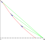
Figure C.1. Illustration of statement (C.1): the mean slope of a certain period is bigger or equal than the mean slope over all later periods

In the $\gamma$ (hotspot source traffic) setting, we know that $N$ is the sender, and thus $\mathcal{A}_{\Lambda}\subset\mathcal{M}_{\Lambda}.$ Hence, we do not need to consider the nodes on the other drop wavelengths and the proof is exactly the same as in the single wavelength case [62], see also figure C.2.

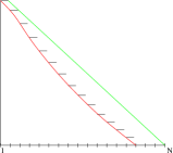
Figure C.2. Gamma setting: the usage probability stays constant on non critical edges

We will now use the same strategy for the more complicated proof in the $\beta$ (hotspot destination traffic) setting. Let $K_{n}$ denote the number of active nodes finding themselves between the nodes $N$ and $n$ (clockwise), i.e.,

(C.3) $$K_{n}:=\left|\mathcal{A}_{\Lambda}\cap\left\{1,\ldots,n-\Lambda\right\}\right|.$$

For $k\in\left\{0,\ldots,\left(n-1\right)\wedge\left(\ell-1\right)\right\}$ we denote $q_{\gamma}^{\ell,k}$ for the probability measure $q_{\gamma}^{\ell}$ conditioned on $K_{n}=k.$ We denote again $n\equiv\delta\Lambda$ for $\delta\in\left\{1,\ldots,\eta-1\right\}$. We will show that

(C.4) $$q_{\beta}^{\ell}\left(n-\Lambda<\mathcal{G}_{\Lambda}\leq n\right)\geq\frac{1}{\eta-\delta}q_{\beta}^{\ell}\left(\mathcal{G}_{\Lambda}>n-\Lambda\right).$$

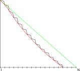
Figure C.3. Beta setting: the usage probability changes along each segment

In case that $S\in\mathcal{M}_{\Lambda}$ we can again use the proof of the one wavelength scenario. This is also true if $S\in\left\{1,\ldots,n-\Lambda\right\}$, since we do not claim anything about these nodes. Hence, we only have to investigate the case $S\in\left\{n-\Lambda+1,\ldots,N\right\}\setminus\mathcal{M}_{\Lambda}$. From now on we assume this to be the case.

We decompose the left hand side into two parts,

(C.5) $$q_{\beta}^{\ell}\left(n-\Lambda<\mathcal{G}_{\Lambda}\leq n\right)=q_{\beta}^{\ell}\left(\mathcal{G}_{\Lambda}=n\right)+q_{\beta}^{\ell}\left(\mathcal{G}_{\Lambda}=S,\,n-\Lambda<S<n\right).$$

For the first summand of (C.5), we proceed similarly to the case of a single wavelength, namely

(C.6) $$q_{\beta}^{\ell,k}\left(\mathcal{G}_{\Lambda}=n\right) = q_{\beta}^{\ell,k}\left(\mathcal{G}_{\Lambda}=n,\,\mathcal{G}_{\Lambda}\geq n,\,\left\lfloor S\right\rfloor_{\Lambda}\neq n,\,n\in\mathcal{F}_{\Lambda}\right)$$

$$= q_{\beta}^{\ell,k}\left(\mathcal{G}_{\Lambda}=n\,\big{|}\,\mathcal{G}_{\Lambda}\geq n,\,\left\lfloor S\right\rfloor_{\Lambda}\neq n,\,n\in\mathcal{F}_{\Lambda}\right)\times$$

$$\times q_{\beta}^{\ell,k}\left(\mathcal{G}_{\Lambda}\geq n\,\big{|}\,\left\lfloor S\right\rfloor_{\Lambda}\neq n,\,n\in\mathcal{F}_{\Lambda}\right)$$

$$\times q_{\beta}^{\ell,k}\left(\left\lfloor S\right\rfloor_{\Lambda}\neq n,\,n\in\mathcal{F}_{\Lambda}\right).$$

We obtain

(C.7) $$q_{\beta}^{\ell,k}\left(\mathcal{G}_{\Lambda}=n\,|\,G\geq n,\,\left\lfloor S\right\rfloor_{\Lambda}\neq n,\,n\in\mathcal{F}_{\Lambda}\right) = q_{\beta,N-n+\Lambda}^{\ell-k}\left(\mathcal{G}_{\Lambda}=1\,|\,\left\lfloor S\right\rfloor_{\Lambda}\neq 1,\,1\in\mathcal{F}_{\Lambda}\right)$$

$$\geq q_{\beta,N-n+\Lambda}^{\ell-k}\left(\mathcal{G}_{\Lambda}^{\leftarrow}=1\,|\,\left\lfloor S\right\rfloor_{\Lambda}\neq 1,\,1\in\mathcal{F}_{\Lambda}\right).$$

This probability can be computed precisely

$$q_{\beta,N-n+\Lambda}^{\ell-k}\left(\mathcal{G}_{\Lambda}^{\leftarrow}=1\,|\,\left\lfloor S\right\rfloor_{\Lambda}\neq 1,\,1\in\mathcal{F}_{\Lambda}\right)$$

$$=q_{\gamma,N-n}^{\ell-k-1}\left(\mathcal{G}_{\Lambda}=0\right)q_{\beta,N-n+\Lambda}^{\ell-k}\left(\left\lfloor S\right\rfloor_{\Lambda}\notin\mathcal{F}_{\Lambda}\,|\,\left\lfloor S\right\rfloor_{\Lambda}\neq 1,\,1\in\mathcal{F}_{\Lambda}\right)+$$

$$\quad+q_{\gamma,N-n}^{\ell-k-2}\left(\mathcal{G}_{\Lambda}=0\right)q_{\beta,N-n+\Lambda}^{\ell-k}\left(\left\lfloor S\right\rfloor_{\Lambda}\in\mathcal{F}_{\Lambda}\,|\,\left\lfloor S\right\rfloor_{\Lambda}\neq 1,\,1\in\mathcal{F}_{\Lambda}\right)$$

$$=\frac{1}{\ell-k}\left(1-\frac{\ell-k-1}{\eta-\delta}\right)+\frac{1}{\ell-k-1}\frac{\ell-k-1}{\eta-\delta}$$

(C.8) $$=\frac{1}{\ell-k}\left(1+\frac{1}{\eta-\delta}\right).$$

We now use the fact that, conditionally on $S\in\left\{n-\Lambda+1,\ldots,N\right\}\setminus\mathcal{M}_{\Lambda}$,

(C.9) $$q_{\beta}^{\ell,k}\left(\left\lfloor S\right\rfloor_{\Lambda}\neq n\in\mathcal{F}_{\Lambda}\right)=q_{\beta}^{\ell,k}\left(\left\lfloor S\right\rfloor_{\Lambda}\neq n\right)q_{\beta}^{\ell,k}\left(n\in\mathcal{F}_{\Lambda}\right)$$

and

(C.10) $$q_{\beta}^{\ell,k}\left(\mathcal{G}_{\Lambda}\geq n\,\big{|}\,\left\lfloor S\right\rfloor_{\Lambda}\neq n\in\mathcal{F}_{\Lambda}\right)=\frac{q_{\beta}^{\ell,k}\left(\mathcal{G}_{\Lambda}\geq n\,\big{|}\,n\in\mathcal{F}_{\Lambda}\right)}{q_{\beta}^{\ell,k}\left(\left\lfloor S\right\rfloor_{\Lambda}\neq n\right)}.$$

Hence, we obtain with $q_{\beta}^{\ell,k}\left(n\in\mathcal{F}_{\Lambda}\right)=\frac{\ell-k-1}{\eta-\delta}$ that

(C.11) $$q_{\beta}^{\ell,k}\left(\mathcal{G}_{\Lambda}=n\right) \geq \frac{1}{\eta-\delta}q_{\beta}^{\ell,k}\left(\mathcal{G}_{\Lambda}\geq n\,\big{|}\,n\in\mathcal{F}_{\Lambda}\right)\times$$

$$\left(1-\frac{1}{\ell-k}\right)\left(1+\frac{1}{\eta-\delta}\right).$$

For the second part of (C.5), we obtain

(C.12) $$q_{\beta}^{\ell,k}\left(\mathcal{G}_{\Lambda}\in I_{\delta}\setminus n\right) = q_{\beta}^{\ell,k}\left(\mathcal{G}_{\Lambda}=S,\,\mathcal{G}_{\Lambda}\geq S,\,\left\lceil S\right\rceil_{\Lambda}=n,\,n\notin\mathcal{F}_{\Lambda}\right)$$

$$= q_{\beta}^{\ell,k}\left(\mathcal{G}_{\Lambda}=S\,\big{|}\,\mathcal{G}_{\Lambda}\geq S,\,\left\lceil S\right\rceil_{\Lambda}=n,\,n\notin\mathcal{F}_{\Lambda}\right)\times$$

$$\times q_{\beta}^{\ell,k}\left(\mathcal{G}_{\Lambda}\geq S\,\big{|}\,\left\lceil S\right\rceil_{\Lambda}=n\notin\mathcal{F}_{\Lambda}\right)q_{\beta}^{\ell,k}\left(\left\lceil S\right\rceil_{\Lambda}=n,\,n\notin\mathcal{F}_{\Lambda}\right).$$

We have

$$q_{\beta}^{\ell,k}\left(\mathcal{G}_{\Lambda}=S\,|\,\mathcal{G}_{\Lambda}\geq S,\,\left\lceil S\right\rceil_{\Lambda}=n,\,n\notin\mathcal{F}_{\Lambda}\right)$$

(C.13) $$=q_{\beta,N-n+\Lambda}^{\ell-k}\left(\mathcal{G}_{\Lambda}=S\,|\,\left\lceil S\right\rceil_{\Lambda}=1,\,1\notin\mathcal{F}_{\Lambda}\right).$$

Now, we use that $\left|\mathcal{A}_{\Lambda}^{\rightarrow}\right|=\left|\mathcal{F}_{\Lambda}+1\right|$ for $\left\lceil S\right\rceil_{\Lambda}\notin\mathcal{F}_{\Lambda}$. Hence, we obtain

$$q_{\beta,N-n+\Lambda}^{\ell-k}\left(\mathcal{G}_{\Lambda}=S\,|\,\left\lceil S\right\rceil_{\Lambda}=1,\,1\notin\mathcal{F}_{\Lambda}\right)$$

$$\geq q_{\beta,N-n+\Lambda}^{\ell-k}\left(\mathcal{G}_{\Lambda}^{\rightarrow}=1\,|\,\left\lceil S\right\rceil_{\Lambda}=1,\,1\notin\mathcal{F}_{\Lambda}\right)$$

$$=q_{\gamma,N-n}^{\ell-k-1}\left(\mathcal{G}_{\Lambda}=0\right)$$

(C.14) $$=\frac{1}{\ell-k}.$$

Note that, conditioned on $S\in\left\{n-\Lambda+1,\ldots,N\right\}\setminus\mathcal{M}_{\Lambda}$, we have

(C.15) $$q_{\beta}^{\ell,k}\left(\left\lceil S\right\rceil_{\Lambda}=n\notin\mathcal{F}_{\Lambda}\right)=q_{\beta}^{\ell,k}\left(\left\lceil S\right\rceil_{\Lambda}=n\right)q_{\beta}^{\ell,k}\left(n\notin\mathcal{F}_{\Lambda}\right)$$

and

(C.16) $$q_{\beta}^{\ell,k}\left(\mathcal{G}_{\Lambda}\geq S\,\big{|}\,\left\lceil S\right\rceil_{\Lambda}=n\notin\mathcal{F}_{\Lambda}\right)=\frac{q_{\beta}^{\ell,k}\left(\mathcal{G}_{\Lambda}\geq S\,\big{|}\,\left\lceil S\right\rceil_{\Lambda}=n\right)}{q_{\beta}^{\ell,k}\left(n\notin\mathcal{F}_{\Lambda}\right)}.$$

Summarizing, we obtain, using $q_{\beta}^{\ell,k}\left(\left\lceil S\right\rceil_{\Lambda}=n\right)=\frac{1}{\eta-\delta}$, that

(C.17) $$q_{\beta}^{\ell,k}\left(\mathcal{G}_{\Lambda}\in I_{\delta}\setminus n\right) \geq \frac{1}{\eta-\delta}\frac{1}{\ell-k}q_{\beta}^{\ell,k}\left(\mathcal{G}_{\Lambda}\geq S\,\big{|}\,\left\lceil S\right\rceil_{\Lambda}=n\right).$$

It remains to show that

(C.18) $$q_{\beta}^{\ell,k}\left(\mathcal{G}_{\Lambda}>n-\Lambda\right) \leq \left(1-\frac{1}{\ell-k}\right)\left(1+\frac{1}{\eta-\delta}\right)\times$$

$$\times q_{\beta}^{\ell,k}\left(\mathcal{G}_{\Lambda}\geq n\,|\,n\in\mathcal{F}_{\Lambda}\right)+$$

$$+\frac{1}{\ell-k}\left(1-\frac{\ell-k-1}{\eta-\delta}\right)\times$$

$$\times q_{\beta}^{\ell,k}\left(\mathcal{G}_{\Lambda}\geq S\,|\,\left\lceil S\right\rceil_{\Lambda}=n,\,n\notin\mathcal{F}_{\Lambda}\right).$$

This can be shown by

$$q_{\beta}^{\ell,k}\left(\mathcal{G}_{\Lambda}>n-\Lambda\right)$$

$$=\sum_{i=\delta}^{\eta-\left(\ell-k\right)}q_{\beta}^{\ell,k}\left(\mathcal{G}_{\Lambda}\geq i\Lambda\,|\,X_{k+1}=i\Lambda\right)q_{\beta}^{\ell,k}\left(X_{k+1}=i\Lambda\right)+$$

$$\qquad+\sum_{\lambda=1}^{\Lambda-1}q_{\beta}^{\ell,k}\left(\mathcal{G}_{\Lambda}\geq i\Lambda-\lambda\,|\,X_{k+1}=i\Lambda-\lambda\right)q_{\beta}^{\ell,k}\left(X_{k+1}=i\Lambda-\lambda\right)$$

$$\leq\left(1-\frac{1}{\ell-k}\right)q_{\beta}^{\ell,k}\left(\mathcal{G}_{\Lambda}\geq n\,|\,X_{k+1}=n\right)+$$

(C.19) $$\quad+\frac{1}{\ell-k}q_{\beta}^{\ell,k}\left(\mathcal{G}_{\Lambda}\geq S\,|\,\left\lceil S\right\rceil_{\Lambda}=n\right).$$

For the last inequality, we used that for $i\in\left\{\delta,\ldots,\eta-1\right\}$ and $\lambda\in\left\{0,\ldots,\Lambda-1\right\}$

$$q_{\beta}^{\ell,k}\left(\mathcal{G}_{\Lambda}\geq i\Lambda-\lambda\,|\,X_{k+1}=i\Lambda-\lambda\right)$$

(C.20) $$\leq q_{\beta}^{\ell,k}\left(\mathcal{G}_{\Lambda}\geq n-\lambda\,|\,X_{k+1}=n-\lambda\right)$$

and, for reasons of symmetry,

(C.21) $$q_{\beta}^{\ell,k}\left(X_{k+1}\in\mathcal{F}_{\Lambda}\right)=1-\frac{1}{\ell-k}.$$

The last step we need is a comparison of (C.18) and (C.19). The only difference arises, when both of the events, $\left\{n\in\mathcal{F}_{\Lambda}\right\}$ and $\left\{\left\lceil S\right\rceil_{\Lambda}=n\right\}$, take place. Then,

(C.22) $$q_{\beta}^{\ell,k}\left(\mathcal{G}_{\Lambda}\geq S\,|\,\left\lceil S\right\rceil_{\Lambda}=n\in\mathcal{F}_{\Lambda}\right)=q_{\beta}^{\ell,k}\left(\mathcal{G}_{\Lambda}\geq n\,|\,\left\lceil S\right\rceil_{\Lambda}=n\in\mathcal{F}_{\Lambda}\right).$$

This occurs with probability $q_{\beta}^{\ell,k}\left(n\in\mathcal{F}_{\Lambda}\,|\,\left\lceil S\right\rceil_{\Lambda}=n\right)=\frac{\ell-k-1}{\eta-\delta}$ and explains the additional factor in the decomposition (C.18). ∎

References

• [1] F. Davik, M. Yilmaz, S. Gjessing, and N. Uzun, “IEEE 802.17 Resilient Packet Ring Tutorial,” IEEE Communications Magazine, vol. 42, no. 3, pp. 112–118, Mar. 2004.
• [2] S. Spadaro, J. Solé-Pareta, D. Careglio, K. Wajda, and A. Szymański, “Positioning of the RPR Standard in Contemporary Operator Environments,” IEEE Network, vol. 18, no. 2, pp. 35–40, March/April 2004.
• [3] P. Yuan, V. Gambiroza, and E. Knightly, “The IEEE 802.17 Media Access Protocol for High-Speed Metropolitan-Area Resilient Packet Rings,” IEEE Network, vol. 18, no. 3, pp. 8–15, May/June 2004.
• [4] N. Ghani, J.-Y. Pan, and X. Cheng, “Metropolitan Optical Networks,” Optical Fiber Telecommunications, vol. IVB, pp. 329–403, 2002.
• [5] J. Fransson, M. Johansson, M. Roughan, L. Andrew, and M. A. Summerfield, “Design of a Medium Access Control Protocol for a WDMA/TDMA Photonic Ring Network,” in Proc., IEEE GLOBECOM, vol. 1, Nov. 1998, pp. 307–312.
• [6] M. A. Marsan, A. Bianco, E. Leonardi, M. Meo, and F. Neri, “MAC Protocols and Fairness Control in WDM Multirings with Tunable Transmitters and Fixed Receivers,” IEEE Journal of Lightwave Technology, vol. 14, no. 6, pp. 1230–1244, June 1996.
• [7] M. A. Marsan, A. Bianco, E. Leonardi, A. Morabito, and F. Neri, “All–Optical WDM Multi–Rings with Differentiated QoS,” IEEE Communications Magazine, vol. 37, no. 2, pp. 58–66, Feb. 1999.
• [8] M. A. Marsan, E. Leonardi, M. Meo, and F. Neri, “Modeling slotted WDM rings with discrete–time Markovian models,” Computer Networks, vol. 32, no. 5, pp. 599–615, May 2000.
• [9] K. Bengi and H. R. van As, “Efficient QoS Support in a Slotted Multihop WDM Metro Ring,” IEEE Journal on Selected Areas in Communications, vol. 20, no. 1, pp. 216–227, Jan. 2002.
• [10] M. Herzog, M. Maier, and M. Reisslein, “Metropolitan Area Packet-Switched WDM Networks: A Survey on Ring Systems,” IEEE Comm. Surveys and Tut., vol. 6, no. 2, pp. 2–20, Second Quarter 2004.
• [11] C. S. Jelger and J. M. H. Elmirghani, “Photonic Packet WDM Ring Networks Architecture and Performance,” IEEE Communications Magazine, vol. 40, no. 11, pp. 110–115, Nov. 2002.
• [12] M. J. Spencer and M. A. Summerfield, “WRAP: A Medium Access Control Protocol for Wavelength–Routed Passive Optical Networks,” IEEE/OSA Journal of Lightwave Technology, vol. 18, no. 12, pp. 1657–1676, Dec. 2000.
• [13] I. M. White, E. S.-T. Hu, Y.-L. Hsueh, K. V. Shrikhande, M. S. Rogge, and L. G. Kazovsky, “Demonstration and system analysis of the HORNET,” IEEE/OSA Journal of Lightwave Technology, vol. 21, no. 11, pp. 2489–2498, Nov. 2003.
• [14] G. Feng, C. K. Siew, and T.-S. P. Yum, “Architectural design and bandwidth demand analysis for multiparty videoconferencing on SONET/ATM rings,” IEEE Journal on Selected Areas in Communications, vol. 20, no. 8, pp. 1580–1588, Oct. 2002.
• [15] R. Beverly and K. Claffy, “Wide-area IP multicast traffic characterization,” IEEE Network, vol. 17, no. 1, pp. 8–15, Jan.-Feb. 2003.
• [16] K. Sarac and K. Almeroth, “Monitoring IP Multicast in the Internet: Recent advances and ongoing challenges,” IEEE Communications Magazine, vol. 43, no. 10, pp. 85–91, Oct. 2005.
• [17] G. N. Rouskas, “Optical layer multicast: rationale, building blocks, and challenges,” IEEE Network, vol. 17, no. 1, pp. 60–65, Jan.-Feb. 2003.
• [18] L. Sahasrabuddhe and B. Mukherjee, “Multicast routing algorithms and protocols: A tutorial,” IEEE Network, vol. 14, no. 1, pp. 90–102, Jan.-Feb. 2000.
• [19] N. Singhal, L. Sahasrabuddhe, and B. Mukherjee, “Optimal multicasting of multiple light-trees of different bandwidth granularities in a WDM mesh network with sparse splitting capabilities,” IEEE/ACM Transactions on Networking, vol. 14, no. 5, pp. 1104–1117, Oct. 2006.
• [20] R. Ul-Mustafa and A. Kamal, “Design and provisioning of WDM networks with multicast traffic grooming,” IEEE Journal on Selected Areas in Communications, vol. 24, no. 4, pp. 37–53, Apr. 2006.
• [21] G.-S. Poo and Y. Zhou, “A new multicast wavelength assignment algorithm in wavelength-routed WDM networks,” IEEE Journal on Selected Areas in Communications, vol. 24, no. 4, pp. 2–12, Apr. 2006.
• [22] S. Sankaranarayanan and S. Subramaniam, “Comprehensive performance modeling and analysis of multicasting in optical networks,” IEEE Journal on Selected Areas in Communications, vol. 21, no. 11, pp. 1399–1413, Nov. 2003.
• [23] J. Wang, X. Qi, and B. Chen, “Wavelength assignment for multicast in all-optical WDM networks with splitting constraints,” IEEE/ACM Transactions on Networking, vol. 14, no. 1, pp. 169–182, Feb. 2006.
• [24] X. Qin and Y. Yang, “Multicast connection capacity of WDM switching networks with limited wavelength conversion,” IEEE/ACM Transactions on Networking, vol. 12, no. 3, pp. 526–538, June 2004.
• [25] A. M. Hamad and A. E. Kamal, “A survey of multicasting protocols for broadcast-and-select single-hop networks,” IEEE Network, vol. 16, no. 4, pp. 36–48, July/August 2002.
• [26] C.-F. Hsu, T.-L. Liu, and N.-F. Huang, “Multicast traffic scheduling in single-hop WDM networks with arbitrary tuning latencies,” IEEE Transactions on Communications, vol. 52, no. 10, pp. 1747–1757, Oct. 2004.
• [27] H.-C. Lin and C.-H. Wang, “A hybrid multicast scheduling algorithm for single–hop WDM networks,” IEEE/OSA Journal of Lightwave Technology, vol. 19, no. 11, pp. 1654–1664, Nov. 2001.
• [28] K. Naik, D. Wei, D. Krizanc, and S.-Y. Kuo, “A reservation-based multicast protocol for WDM optical star networks,” IEEE Journal on Selected Areas in Communications, vol. 22, no. 9, pp. 1670–1680, Nov. 2004.
• [29] X. Zhang and C. Qiao, “On Scheduling All-to-All Personalized Connections and Cost-Effective Designs in WDM Rings,” IEEE/ACM Transactions on Networking, vol. 7, no. 3, pp. 435–445, June 1999.
• [30] O. Gerstel, R. Ramaswami, and G. H. Sasaki, “Cost-Effective Traffic Grooming in WDM Rings,” IEEE/ACM Transactions on Networking, vol. 8, no. 5, pp. 618–630, Oct. 2000.
• [31] J. Wang, W. Cho, V. R. Vemuri, and B. Mukherjee, “Improved Approaches for Cost-Effective Traffic Grooming in WDM Ring Networks: ILP Formulations and Single-Hop and Multihop Connections,” IEEE/OSA Journal of Lightwave Technology, vol. 19, no. 11, pp. 1645–1653, Nov. 2001.
• [32] L.-W. Chen and E. Modiano, “Efficient Routing and Wavelength Assignment for Reconfigurable WDM Ring Networks With Wavelength Converters,” IEEE/ACM Transactions on Networking, vol. 13, no. 1, pp. 173–186, Feb. 2005.
• [33] D.-R. Din, “Genetic algorithms for multiple multicast on WDM ring network,” Computer Communications, vol. 27, no. 9, pp. 840–856, June 2004.
• [34] I. Ferrel, A. Mettler, E. Miller, and R. Libeskind-Hadas, “Virtual topologies for multicasting with multiple originators in WDM networks,” IEEE/ACM Transactions on Networking, vol. 14, no. 1, pp. 183–190, Feb. 2006.
• [35] X. Jia, X.-D. Hu, L. Ruan, and J. Sun, “Multicast routing, load balancing, and wavelength assignment on tree of rings,” IEEE Communications Letters, vol. 6, no. 2, pp. 79–81, Feb. 2002.
• [36] R. Libeskind-Hadas, J. R. Hartline, K. Dresner, E. Drucker, and K. Ray, “Multicast virtual topologies in WDM paths and rings with splitting loss,” in Proc. Int. Conf. on Computer Communications and Networks, Oct. 2002, pp. 318–321.
• [37] J. Wang, B. Chen, and R. Uma, “Dynamic wavelength assignment for multicast in all-optical WDM networks to maximize the network capacity,” IEEE Journal on Selected Areas in Communications, vol. 21, no. 8, pp. 1274–1284, Oct. 2003.
• [38] C. Zhou and Y. Yang, “Wide–sense Nonblocking Multicast in a Class of Regular Optical WDM Networks,” IEEE Transactions on Communications, vol. 50, no. 1, pp. 126–134, Jan. 2002.
• [39] M. Veeraraghavan, H. Lee, J. Anderson, and K. Y. Eng, “A network throughput comparison of optical metro ring architectures,” in Proc., OFC, Mar. 2002, pp. 763–765.
• [40] A. Carena, V. D. Feo, J. M. Finochietto, R. Gaudino, F. Neri, C. Piglione, and P. Poggiolini, “RingO: An Experimental WDM Optical Packet Network for Metro Applications,” IEEE Journal on Selected Areas in Communications, vol. 22, no. 8, pp. 1561–1571, Oct. 2004.
• [41] M. A. Marsan, A. Bianco, E. Leonardi, M. Meo, and F. Neri, “On the Capacity of MAC Protocols for All–Optical WDM Multi–Rings with Tunable Transmitters and Fixed Receivers,” in Proc., IEEE INFOCOM, vol. 3, Mar. 1996, pp. 1206–1216.
• [42] J. He, S.-H. G. Chan, and D. H. K. Tsang, “Multicasting in WDM Networks,” IEEE Communications Surveys and Tutorials, vol. 4, no. 1, Third Quarter 2002.
• [43] M. Boroditsky, C. F. Lam, S. L. Woodward, N. J. Frigo, and M. D. Feuer, “Power management for enhanced system performance of passive optical rings,” IEE Proceedings Optoelectronics, vol. 150, no. 3, pp. 229–234, June 2003.
• [44] S. Aleksic and K. Bengi, “Multicast-capable access nodes for slotted photonic ring networks,” in Proc. European Conference on Optical Communications (ECOC), Sept. 2000, pp. 83–84.
• [45] E. Shimada, S. Fujiwara, K. Okazaki, and I. Sasase, “A transmission system for multicast traffic with preallocation scheme in WDM ring networks,” in Proc. IEEE Pacific Rim Conf. on Comm., Computers and Signal Proc., Aug. 2003, pp. 490–493.
• [46] C. Piglione, M. Reisslein, and F. Neri, “Fair uni- and multicasting in a ring metro WDM network,” OSA Journal of Optical Networking (JON), vol. 3, no. 8, pp. 601–622, 2004.
• [47] M. Chaitou, G. Hebuterne, and H. Castel, “Performance of multicast in WDM slotted ring networks,” Computer Communications, vol. 30, no. 2, pp. 219–232, Jan. 2007.
• [48] M. Scheutzow, P. Seeling, M. Maier, and M. Reisslein, “Multicasting in a WDM-upgraded Resilient Packet Ring,” OSA Journal of Optical Networks, vol. 6, no. 5, pp. 415–421, May 2007.
• [49] M. Scheutzow, M. Reisslein, M. Maier, and P. Seeling, “Multicast Capacity of Packet-Switched Ring WDM Networks,” IEEE Transactions on Information Theory, vol. 54, no. 2, pp. 623–644, Feb. 2008.
• [50] H. Zähle and M. Scheutzow and M. Reisslein and M. Maier, “On the multicast capacity of unidirectional and bidirectional packet-switched WDM ring networks,” IEEE Journal on Selected Areas in Communications, vol. 25, no. 4, pp. 105–119, Apr. 2007.
• [51] A. A. M. Saleh and J. M. Simmons, “Architectural Principles of Optical Regional and Metropolitan Access Networks,” IEEE/OSA Journal of Lightwave Technology, vol. 17, no. 12, pp. 2431–2448, Dec. 1999.
• [52] R. Berry and E. Modiano, “Optimal Transceiver Scheduling in WDM/TDM Networks,” IEEE Journal on Selected Areas in Communications, vol. 23, no. 8, pp. 1479–1495, Aug. 2005.
• [53] H. Liu and F. A. Tobagi, “Traffic grooming in WDM SONET UPSR rings with multiple line speeds,” in Proc., IEEE INFOCOM, Mar. 2005, pp. 718–729.
• [54] X.-Y. Li, P.-J. Wan, and L. Liu, “Select line speeds for single-hub SONET/WDM ring networks,” in Proc., IEEE Int. Conf. on Communications, June 2000, pp. 495–499.
• [55] S. Subramaniam, M. Azizoglu, and A. Somani, “On the optimal placement of wavelength converters in wavelength-routed networks,” in Proc., IEEE INFOCOM, Mar. 1998, pp. 902–909.
• [56] J. Wang, W. Cho, V. R. Vemuri, and B. Mukherjee, “Improved approaches for cost-effective traffic grooming in WDM ring networks: ILP formulations and single-hop and multihop connections,” IEEE/OSA Journal of Lightwave Technology, vol. 19, no. 11, pp. 1645–1653, Nov. 2001.
• [57] Y. Xu and X. Yao, “Lower bound on number of ADMs in WDM rings with nonuniform traffic demands,” Electronics Letters, vol. 40, no. 13, pp. 824–825, June 2004.
• [58] X. Zhang and C. Qiao, “An Effective and Comprehensive Approach for Traffic Grooming and Wavelength Assignment in SONET/WDM Rings,” IEEE/ACM Transactions on Networking, vol. 8, no. 5, pp. 608–617, Oct. 2000.
• [59] A. Zapata, M. Duser, J. Spencer, P. Bayvel, I. deMiguel, D. Breuer, N. Hanik, and A. Gladisch, “Next-generation 100-gigabit metro ethernet (100 GbME) using multiwavelength optical rings,” IEEE/OSA Journal of Lightwave Technology, vol. 22, no. 11, pp. 2420–2434, Nov. 2004.
• [60] I. Rubin and H. Hua, “Synthesis and throughput behaviour of WDM meshed-ring networks under nonuniform traffic loading,” IEEE/OSA Journal of Lightwave Technology, vol. 15, no. 8, pp. 1513–1521, Aug. 1997.
• [61] M. Chaitou, G. Hebuterne, and H. Castel, “Modelling multi-channel optical slotted rings with fixed transmitter and fixed receivers,” in Proc., Advanced Industrial Conference on Telecommunications/Service Assurance with Partial and Intermittent Resources Conference/ E-Learning on Telecommunications Workshop, July 2005, pp. 115–120.
• [62] M. an der Heiden, M. Sortais, M. Scheutzow, M. Reisslein, P. Seeling, M. Herzog, and M. Maier, “Multicast Capacity of Optical Packet Ring for Hotspot Traffic,” IEEE/OSA Journal of Lightwave Technology, vol. 25, no. 9, pp. 2638–2652, Sept. 2007.
• [63] M. Maier, M. Scheutzow, M. Herzog, and M. Reisslein, “Multicasting in IEEE 802.17 Resilient Packet Ring,” OSA Journal of Optical Networks, vol. 5, no. 11, pp. 841–857, Nov. 2006.
• [64] A. Bianco, J. M. Finochietto, G. Giarratana, F. Neri, and C. Piglione, “Measurement-based reconfiguration in optical ring metro networks,” IEEE/OSA Journal of Lightwave Technology, vol. 23, no. 10, pp. 3156–3166, Oct. 2005.
• [65] H. Elbiaze and O. Cherkaoui, “Exploiting self-similar traffic analysis in network resource control: the IP over WDM networks case,” in Proc., IEEE Int. Conf. on Autonomic and Autonomous Systems and Int. Conf. on Networking and Services (ICAS-ICNS), Oct. 2005, pp. 65–71.
• [66] A. Elwalid, D. Mitra, I. Saniee, and I. Widjaja, “Routing and protection in GMPLS networks: from shortest paths to optimized designs,” IEEE/OSA Journal of Lightwave Technology, vol. 21, no. 11, pp. 2828–2838, Nov. 2003.
• [67] A. Gencata and B. Mukherjee, “Virtual-topology adaptation for WDM mesh networks under dynamic traffic,” IEEE/ACM Transactions on Networking, vol. 11, no. 2, pp. 236–247, Apr. 2003.
• [68] E. Oki, K. Shiomoto, S. Okamoto, W. Imajuku, and N. Yamanaka, “Heuristic multi-layer optimum topology design scheme based on traffic measurement for IP + photonic networks,” in Proc., Optical Fiber Communication Conference and Exhibit (OFC), Mar. 2002, pp. 104–105.