Constraining the mSUGRA parameter space using the entropy of dark matter halos

Abstract

We derive an expression for the entropy of a dark matter halo described by a Navarro-Frenk-White model with a core. The comparison of this entropy with the one of dark matter at the freeze-out era allows us to constraint the parameter space in mSUGRA models. Moreover, joining these constraints with the ones obtained from the usual abundance criteria and demanding both criteria to be consistent with the 2$\sigma$ bounds for the abundance of dark matter: $0.112\leq\Omega_{DM}h^{2}\leq 0.122$, we are able to clearly discriminate validity regions among the values of $\tan\beta$, one of the parameters of the mSUGRA model. We found that for the explored regions of the parameter space, small values of tan$\beta$ are not favored; only for tan$\beta\simeq 50$ are both criteria significantly consistent. In the region where both criteria are consistent we also found a lower bound for the neutralino mass, $m_{\chi}\geq 141$ GeV.

, , , , and

keywords: dark matter, cosmology of theories beyond the SM, structure of galaxies

1 Introduction

The existence of components of the total energy-density of the Universe whose nature is still not understood, constitutes one of the biggest unsolved questions in physics today. It is a great challenge to have a clear picture of the nature of dark matter (DM), and dark energy, whose existence is more and more undisputed with the observational evidence accumulated over the last decades.

The observational constraints on the present density of DM, $\Omega_{DM}$, come from several outstanding observations such as the Cosmic Microwave Background radiation (CMBR) [1], galaxy clustering, supernovae and Lyman $\alpha$ forest. One of the most recent works which combines all these data leads to: $0.112\leq\Omega_{DM}h^{2}\leq 0.122$ [2], with $h$ the dimensionless value of the present day Hubble constant ($h\sim 0.7$). These bounds imply that dark matter constitutes $22.8-24.8\,\%$ of the total density of the Universe.

One of the most accepted candidates to be the major component of dark matter is the neutralino as the Lightest Supersymmetric Particle (LSP). Supersymmetric theories with R-parity conservations predict this particle (for an excellent introduction to Supersymmetry see [3]). This type of models have several parameters, some of which can be constrained by combining different methods with observational data of the actual density of DM. In particular for mSUGRA models, this has been done using a standard approach [4, 5], based on solving the Boltzmann equation by considering that after the “freeze-out” era, neutralinos cease to annihilate keeping its number constant. In such approach, the relic density of neutralinos is approximately given by (this is strictly true only when $\langle\sigma v\rangle$ is independent of the energy):

$$\Omega_{\chi}\propto 1/\langle\sigma v\rangle,$$ (1)

where $\langle\sigma v\rangle$ is the thermally averaged cross section times the Moller velocity of the annihilating pair.

Within the mSUGRA model, five parameters are needed to specify the supersymmetric spectrum of particles and the final relic density of the LSP. These parameters are: $m_{0}$, the unified mass for scalars, $m_{1/2}$, the unified mass for gauginos, $A_{0}$, the unified trilinear coupling, tan$\beta$, the ratio of the vacuum expectation values of the neutral components of the supersymmetric Higgs bosons and the sign of $\mu$, where $\mu$ is the Higgsino mass parameter. In this work we use the numerical code micrOMEGAs [6] to compute the LSP’s relic density for different values of these parameters. This scheme will be called hereafter the “abundance criterion” (AC), which combined with the hypothesis $\Omega_{DM}=\Omega_{\chi}$, gives an effective way to constraint the values of those five parameters.

Another estimate for $\Omega_{\chi}$ can be obtained using a different approach. Just before the “freeze-out” epoch, we can consider neutralinos as forming a Maxwell-Boltzmann (MB) gas in thermal equilibrium with the rest of the components of the Universe. In the present time, such a gas is almost collisionless and either constitutes galactic halos and larger structures or it is in the process of their formation. In this context, we can conceive two equilibrium states for the neutralino gas, the decoupling (or “freeze-out”) epoch and its present state as a virialized system. Computing the entropy per particle for each one of these states, we can use an “entropy consistency” criterion (EC), based on the comparison of theoretical and empirical estimates for this entropy, to obtain an alternative expression for the relic density of neutralinos $\Omega_{\chi}$, functionally dependent of the mSUGRA parameters. This idea was originally introduced by some of us in [7].

Our objective is then to develop the recently introduced EC, as a complementary method to the well known AC, in order to obtain further constraints on the parameters of the mSUGRA model by demanding consistency of both criteria with each other and with the observational constraints on $\Omega_{DM}$ (preliminary results of this analysis were already presented in [8]).

The paper is organized as follows, in section II we present a brief description of the method to compute $\Omega_{\chi}$ using the AC. In section III a derivation of the EC is explained. In section IV we present the halo model together with a detailed description of the method we followed to obtain one of the key empirical parameters in the EC. In section V we present the results obtained by comparing both criteria with the observational constraints on $\Omega_{DM}$ in the context of the mSUGRA model. In the last section a summary and the conclusions of our work are presented.

2 Abundance criterion

The relic abundance of neutralinos is defined as $\Omega_{\chi}=\rho_{\chi}/\rho_{crit}$, where $\rho_{\chi}=m_{\chi}n_{\chi}$ is the relic’s mass density ($n_{\chi}$ is the number density, $m_{\chi}$ the neutralino mass) and $\rho_{crit}$ is the critical density of the Universe (see [9] for a review on the following method to compute the relic density). The time evolution of $n_{\chi}$ is given by the Boltzmann equation:

$$\frac{dn_{\chi}}{dt}=-3Hn_{\chi}-\langle\sigma v\rangle(n_{\chi}^{2}-(n_{\chi}^{eq})^{2}),$$ (2)

where $H$ is the Hubble expansion rate and $n_{\chi}^{eq}$ is the number density of neutralinos in thermal equilibrium. In the early Universe, neutralinos and the rest of species were in thermal equilibrium, that is $n_{\chi}=n_{\chi}^{eq}$. As the Universe expanded, their typical interaction rate started to diminish and the process of annihilation froze out. Since then, the global comoving number density of neutralinos has remained nearly constant.

There are several ways to solve Eq. (2). The most common approach is based on the “freeze-out” approximation (see for example [10]). If we consider that neutralinos are the major component of the dark matter density, $\Omega_{\chi}\approx\Omega_{DM}$, then the freeze-out approximation gives a functional dependence between $\Omega_{DM}$ and the mSUGRA parameters. In other words, it gives a constraint equation for these parameters.

In practice, however, we obtain a numerical solution to the Boltzmann equation, Eq. (2), using the public code micrOMEGAs 1.3.6 [6], this gives us better precision over the usual freeze-out approximation. The code computes the relic density of the LSP in the Minimal Supersymmetric Standard Model (MSSM), taking into account all annihilation and coannihilation processes as well as loop-corrected masses and mixings to calculate $\langle\sigma v\rangle$ exactly. Further on, we take the mSUGRA model and its five parameters ($m_{0}$, $m_{1/2}$, $A_{0}$, tan$\beta$ and the sign of $\mu$) as input for micrOMEGAs and use Suspect in its version 2.34 [11], which comes as an interface to micrOMEGAs, to calculate the supersymmetric mass spectrum of particles.

Using this criterion, we can obtain the allowed regions in the parameter space of the mSUGRA model which are consistent with observational constraints on the actual dark matter density.

3 Entropy consistency criterion

This criterion was originally introduced in [7]. We briefly describe it in the following.

The main idea of the method is to compare the neutralino gas in two stages of its evolution as the Universe evolved, namely, the freeze-out era and the present epoch. These initial and final states are taken as equilibrium states. In this approach we disregard the complex phenomena that took place during the formation and evolution of structure in the Universe, and the analysis is focused only on those two stages. In the freeze-out era, the assumption is to treat the neutralino gas as a non-relativistic ideal gas of WIMPs (weakly interacting massive particles) described by Maxwell-Boltzmann statistics. This assumption is valid mainly because in this era, the dominant interactions in the gas are still short-ranged and neutralinos are already non-relativistic by then ($m_{\chi}\gtrsim 100$ GeV).

We would like to apply the MB description for present day structures as well, in particular to galactic halos, which we consider as final states of the primordial neutralino gas. However, the valid assumptions made for the freeze-out era are no longer valid for such final states, because in galactic halos, neutralinos are mainly subject to long-range interactions, related to non-extensive forms of energy and entropy. Following the guidelines given in [7], a more general approach can be applied instead, it uses the microcanonical ensemble in the “mean field” approximation. This approach is actually valid at both, the initial and final stages. The state of the system in each state is defined by its entropy per particle s, its density n, and its temperature T; the latter is actually given by the auxiliary variable $x=\frac{m_{\chi}}{T}$. This set of variables is then ($s_{\hbox{f}},\,x_{\hbox{f}},\,n_{\hbox{f}}$) for the neutralino gas at the freeze-out era and ($s^{\hbox{\tiny{(h)}}},\,x^{\hbox{\tiny{(h)}}},\,n^{\hbox{\tiny{(h)}}}$) for the dark matter halo today. Therefore, the change in entropy per particle between these two states is given by:

$$s^{\hbox{\tiny{(h)}}}\ -\ s_{\hbox{f}}\ =\ \ln\,\left[\frac{n_{\hbox{f}}}{n^{\hbox{\tiny{(h)}}}}\left(\frac{x_{\hbox{f}}}{x^{\hbox{\tiny{(h)}}}}\right)^{3/2}\right].$$ (3)

The region today in which all these considerations apply is the center of galactic halos. Thus, in what follows, we consider current halo macroscopic variables as evaluated in this region: $s_{c}^{\hbox{\tiny{(h)}}},\,x_{c}^{\hbox{\tiny{(h)}}},\,n_{c}^{\hbox{\tiny{(h)}}}$.

We can then write $s_{c}^{\hbox{\tiny{(h)}}}$ using Eq. (3) as an equation depending only on present day values of certain quantities, such as the ratio of the total density of the Universe to $\rho_{crit}$, $\Omega_{0}$, and the value of the freeze-out temperature of the neutralino gas. This was done in detail in [7] and the result can be written as:

$$s_{c}^{\hbox{\tiny{(h)}}}|_{{}_{\hbox{\tiny{th}}}}=\frac{5}{2}+x_{\hbox{f}}+\ln\left[\frac{g_{*\hbox{f}}\left(x_{\hbox{f}}\right)\left(x_{0}^{\hbox{\tiny{CMB}}}\right)^{3}}{g_{*0}\left(x_{0}^{\hbox{\tiny{CMB}}}\right)}\frac{h^{2}\,\Omega_{0}}{(x_{\hbox{f}}\,x_{c}^{\hbox{\tiny{(h)}}})^{3/2}}\,\frac{\rho_{crit}}{\rho_{c}^{\hbox{\tiny{(h)}}}}\right].$$ (4)

where $g_{*}$ is related to the degrees of freedom of the system, $x_{0}^{\hbox{\tiny{CMB}}}\equiv m_{\chi}/T_{0}^{\hbox{\tiny{CMB}}}=4.29\times 10^{12}\,m_{\chi}/\hbox{GeV}$, with $T_{0}^{\hbox{\tiny{CMB}}}=2.7\,\hbox{K}$ (see [10] for details).

It is important to mention that there is an alternative formalism to study autogravitating systems such as dark matter halos. It is based on a non-extensive description of energy and entropy developed by Tsallis [12]. Such formalism was applied to dark matter halos and compared with the predominant $\Lambda$CDM paradigm obtaining suggestive results [13, 14]. However, for the purposes of this work we will continue with the traditional formalism.

If the neutralino gas in present halo structures would strictly satisfy MB statistics, the entropy per particle would follow from the well known Sackur–Tetrode entropy formula [15]. Such a MB gas in equilibrium would be equivalent to an isothermal halo if we make the connection [16]: $\sigma_{\hbox{\tiny{(h)}}}^{2}=k_{{}_{B}}T^{\hbox{\tiny{(h)}}}/m$, where $\sigma_{\hbox{\tiny{(h)}}}^{2}$ is the velocity dispersion (a constant for isothermal halos). However, as mentioned before, the assumption of MB statistics does not apply for self–gravitating collisionless systems. Hence, an exactly isothermal halo is not a realistic model, not only because of these theoretical arguments, but also because its total mass diverges and its distribution function allows for infinite particle velocities (theoretically accessible in the velocity range of the MB distribution).

More realistic halo models follow from “energy truncated” distribution functions [16]-[20] that assume a maximal “cut off” velocity (an escape velocity). Therefore, we can provide a convenient empirical estimate of the halo entropy, $s_{c}^{\hbox{\tiny{(h)}}}$, following the microcanonical definition of entropy in terms of the allowed phase space volume, restricted to the range of velocities accessible to the central particles, that is up to a maximal escape velocity $v_{e}(0)$. If we reasonably assume that:

$$v_{e}^{2}(0)\ =\ 2\,|\Phi(0)|\ \simeq\ \alpha\,\sigma_{\hbox{\tiny{(h)}}}^{2}(0),$$ (5)

where $\Phi(r)$ is the Newtonian gravitational potential, and $\alpha$ is a proportionality constant, then we can write:

$$s_{c}^{\hbox{\tiny{(h)}}}|_{{}_{\hbox{\tiny{em}}}}\ \simeq\ln\left[\frac{m^{4}\,v_{e}^{3}}{(2\pi\hbar)^{3}\,\rho_{c}^{\hbox{\tiny{(h)}}}}\right]=89.17+\ln\left[\left(\frac{m}{\hbox{GeV}}\right)^{4}\,\left(\frac{\alpha}{x^{\hbox{\tiny{(h)}}}_{c}}\right)^{3/2}\,\frac{\hbox{GeV/cm}^{3}}{\rho_{c}^{\hbox{\tiny{(h)}}}}\right]$$

where we used $x_{c}^{\hbox{\tiny{(h)}}}=c^{2}/\sigma_{\hbox{\tiny{(h)}}}^{2}(0)$ with $c$ the speed of light.

Equating the theoretical and empirical estimates for the entropy per particle (Eqs. (4) and (3)) we finally obtain a relation for the relic abundance of neutralinos (this formula is a small modification of the one presented in [7]):

$$\textrm{ln}(\Omega_{\chi}h^{2})=10.853-x_{\hbox{f}}+\textrm{ln}\left[\frac{(x_{\hbox{f}}\alpha)^{3/2}m_{\chi}g_{*0}\left(x_{0}^{\hbox{\tiny{CMB}}}\right)}{g_{*\hbox{f}}\left(x_{\hbox{f}}\right)}\right]$$ (6)

In this way we have obtained another constraint equation for the parameters of the mSUGRA model (recall that $\Omega_{DM}=\Omega_{\chi}$).

In order to perform an analysis of the mSUGRA parameters using this new entropy criterion, we modified micrOMEGAs to compute the value of $x_{\hbox{f}}$ for any region of the parameter space, and then compute $\Omega_{\chi}$ using Eq. (6). We can then find the subspace of values of the mSUGRA parameters consistent with the observed constraints on the dark matter density.

The extra parameter $\alpha$ in Eq. (6), which is the proportionality factor between the escape and dispersion velocities at the halo center has a major role in our work. It is very important for the EC that we are able to give values to $\alpha$ in an independent way. In the following section, we show in detail how this parameter can be evaluated for a particular dark matter halo model.

The scheme we have developed so far is only for dark matter particles, namely neutralinos. We have not included at any moment the baryons which constitute the galaxies that we observe today. As we discuss further on, this condition makes our method strictly valid only for pure dark matter structures and gives a reasonable approximation when the dynamical effects of baryons can be neglected. The main effects coming from the addition of baryons that should be included in our model are: i) neutralino-nucleon elastic scattering interactions and ii) gravitational effects from the baryonic component onto the dark matter halo. Although both of these effects are more significant in the central region of the halos, precisely where our method should be applied, we believe that the latter can be avoided if we focus our analysis on systems where the baryon-to-dark mass content is significantly low, and the former can be safely neglected in all cases since the interaction rate between neutralinos and baryons is highly suppressed by the low neutralino-proton scattering cross section predicted by theoretical models $~{}10^{-44}-10^{-45}$ cm² (see for example [38], see also [39] for recent experimental upper limits). The formation of a baryonic component in the galactic (halo+baryons) system, a disc for example, modifies the original mass distribution of dark matter, the effect is a net contraction of the halo towards the center, see for example [44] for a classical description on how to include this effect. In what follows we will not consider it though, since we will focus on dark matter dominated systems where the effect is less significant.

4 About the parameter $\alpha$

The formula for the entropy per particle in the center of halos, Eq. (3), is far from being the final description from a statistical-mechanics point of view. The question about the actual description governing “dark matter fluids” remains open. Nevertheless, it is the assumption we have made about the neutralino gas, taking it nearly as an ideal gas, that make Eq. (3) consistent. In fact, other works in the past have considered the approximation of dark matter as an ideal gas as the approach to follow when it comes to analyzing the entropy (see for example [40], [41]). Our ignorance on the correct statistical-mechanics treatment for systems formed by dark matter is reflected in the appearance of the parameter $\alpha$ in Eq. (3). It is of key importance to find appropriate bounds for its value. In the following, we present an specific model used to obtain estimates for such bounds. We have chosen this model trying to balance simplicity with an approximate general description of dark matter halos.

The model consists of an spherical dark matter halo with a constant density core in the center, beyond which the dark matter density profile follows the well known Navarro-Frenk-White (NFW) profile [42], we set a cut-off radius to define the halo boundary:

$$\rho(y)=\left\{\begin{array}[]{ll}\rho_{c}&\textrm{if $y<y_{c}$}\\ \frac{\delta_{0}\rho_{0}}{y(1+y)^{2}}&\textrm{if $y_{c}\leq y\leq y_{v}$}\\ 0&\textrm{if $y>y_{v}$}\end{array}\right.$$

    (7)

where $\rho_{c}$ is the constant central density of the core, $y=r/r_{s}$, $y_{c}=r_{c}/r_{s}$, $y_{v}=r_{v}/r_{s}$, $r_{s}$ is a scale radius, $r_{c}$ is the core radius and $r_{v}$ is the virial radius, which defines the limit for the virialized structure; $\rho_{0}$, $\delta_{0}$ and $r_{s}$ are the usual parameters of the the NFW profile. The choice of an NFW profile for the external part is clearly motivated by the success of the profile as a universal fit to dark matter halos in numerical simulations. The central core is motivated by the apparent need of it in dark matter dominated systems, see further below, and also by the phenomenon of dark matter annihilation which could produce it naturally (see for example [43]).

For a model without core, all these parameters can be given by a series of well-established formulas (see for example [14, 42, 44, 45]):

$$\delta_{0}=\frac{\Delta\,c^{3}}{3\left[\ln\,(1+c)-c/(1+c)\right]},$$ (8)

$$\rho_{0}=\rho_{\mathrm{crit}}\,\Omega_{0}\,h^{2}=277.8\,h^{2}\,\frac{M_{\odot}}{\rm{kpc}^{3}},$$ (9)

where $c=r_{s}/r_{v}$ is the concentration parameter. We choose a $\Lambda$CDM model with $\Omega_{0}=1,\Omega_{\Lambda}=0.7$, which seems to be in accordance with different sources of observations [1]; and $\Delta\sim 100$ [46, 47].

With Eqs. (8) and (9) and the definition of the parameter $c$, the NFW density profile is defined by two parameters only, a “size” parameter ($r_{s}$ or $r_{v}$) and the concentration parameter $c$. In fact, both can be written in terms of the total mass of the halo, $M_{v}$:

$$r_{v}=\left(\frac{3M_{v}}{4\pi\Delta\rho_{0}}\right)^{1/3},$$ (10)

$$c_{0}\approx 160\left(\frac{M_{v}h}{M_{\odot}}\right)^{-0.096}.$$ (11)

Eq. (11) is a fit extracted from the numerical study [48], which is based on the Millennium simulation data [49], the sample of relaxed halos presented in that work was chosen as more appropriate for our purposes (the halos in this sample are closer to virial equilibrium). The results were transformed from the original value $\Delta=200$ to $\Delta=100$, to do so, we used the code provided by the authors. Other studies in the past have found different fitting formulas for the mass-concentration relation, we believe our results are not highly sensitive to a specific formula (we actually tested this with the formula used in[50]). Eq. (11) however, just gives a central value for the concentration (this is why we use the term $c_{0}$ to represent it), actually, the relation between $c$ and $M_{v}$ in numerical studies has a scatter, $\sigma_{logc}$, which is slightly dependent on $M_{v}$ itself. For the remainder of this work, we take however the same value for all halos, given by the mean of $\sigma_{logc}$ for the sample of relaxed halos presented in [48] (see table 1 of their paper): $\sigma_{logc}\approx 0.095$.

Using Eqs. (8-11) together with the NFW density profile, without core, we have a model that can in principle be used to describe dark matter structures with only one free parameter: $M_{v}$. A particular case can always deviate from this average model mostly because of the scatter in the concentration parameter $c$. This situation can be alleviated if one takes into account the expected range of values for $c$ given by $\sigma_{logc}\approx 0.095$ as described above.

Such description is, however, not valid for all dark matter halos. There is specially a controversy, still not resolved, of whether or not all galaxies are consistent with the cuspy behavior of the NFW profile in the center. For dwarf and low surface brightness (LSB) galaxies there seems to be a disagreement [51]-[56]. On the other hand, for large structures like galaxy clusters, the NFW description is strongly supported by observations [57]-[59]. Recent numerical simulations are able to resolve regions closer to the center of dark matter halos and seem to favor even cuspier density profiles. For example in [60], $\rho\sim r^{-\gamma}$ with $\gamma\sim$ 1.1, 1.2 and 1.35 for cluster-, galaxy- and dwarf-size halos respectively, another analysis ([61]) finds $\gamma\sim 1.2$ for a cluster-size halo. Both analysis agree that a model with a core underestimates the simulated dark matter density within the resolution limits of each work, this limit is roughly 1 percent of the virial radius. The estimates for the parameter $\alpha$ that we obtain further on are still consistent with these numerical results since the values for the core radius that we find for our model are slightly inside this resolution limit.

For the purposes of our analysis, and given the hypothesis we have made, we are interested in structures that are dominated by dark matter, that is, that the baryonic or visible component is less representative and has no important global effects. In fact, in order to empirically estimate the entropy of dark matter halos, we have neglected the effects of the luminous galaxies within them, thus, our model should be in principle formally valid only for structures that are made exclusively of dark matter. Dark matter dominated systems, like dwarf and LSB galaxies, whose dynamics is close to systems which only have dark matter, will be taken as a reference to put bounds on the parameter $\alpha$. Taking into account the information we have on such systems, the choice of a halo model with the same properties of an NFW profile in the external region, but with a core in the central region, seems to be reasonable.

We consider Eqs. (8-11) to be valid as well for this model. Such assumption is strictly valid for Eqs. (8-9) because they refer only to a particular way to define the normalization of the profile, they can be used as long as one takes into account its connection to the central density: $\delta_{0}\rho_{0}/(y_{c}(1+y_{c})^{2})=\rho_{c}$. The same reasoning is valid for Eq. (10), which is independent of the particular model for the density profile, it is a definition for virialized spherical systems depending only on the cosmological model. Eq. (11) is valid only as an approximation, the virial mass appearing on it refers strictly to the virial mass computed for an NFW model without core, the introduction of the core reduces the mass in a percentage that depends on how large is $r_{c}$. However, for low values of $r_{c}$ compared to $r_{v}$, the difference caused by the core is not relevant and the formula can be taken as a good approximation. In any case, Eq. (11) can be always considered as a fair way to give a value to one of the free parameters ($c$ or $r_{s}$) in the model.

With all the previous considerations, we can continue and calculate analytically the parameter $\alpha$. First, the mass profile for our model follows from Eq. (7):

$$M(y)=\left\{\begin{array}[]{ll}\frac{4}{3}\pi\rho_{c}r_{s}^{3}y^{3}&\textrm{if $y<y_{c}$}\\ \frac{r_{s}}{G}V_{0}^{2}\left(\frac{y_{c}(4y_{c}+3)}{3(1+y_{c})^{2}}+ln\left(\frac{1+y}{1+y_{c}}\right)-\frac{y}{1+y}\right)&\textrm{if $y_{c}\leq y\leq y_{v}$}\\ \end{array}\right.$$

    (12)

where $V_{0}^{2}=4\pi Gr_{s}^{2}\delta_{0}\rho_{0}$ and $G=4.297\times 10^{-6}(\textrm{km/s})^{2}\textrm{kpc}/M_{\odot}$ is the gravitational constant in appropriate units (here we have followed closely the work [62]). Using the mass profile, we calculate the gravitational potential at $r=0$, $\Phi(0)$: $d\Phi(r)/dr=GM(r)/r^{2}$; we use also the fact that $\Phi(r_{v})=-GM(r_{v})/r_{v}$ ($\rho=0$ for $r>r_{v}$), we obtain:

$$\Phi(0)=V_{0}^{2}\left(\frac{1}{1+y_{v}}-\frac{3y_{c}+2}{2(1+y_{c})^{2}}\right).$$ (13)

In order to calculate the velocity dispersion in the center, $\sigma(0)$, we use the Jeans equation for spherical systems [16, 45]:

$$\frac{1}{\rho}\frac{d(\rho\bar{v_{r}^{2}})}{dr}+2\frac{B\bar{v_{r}^{2}}}{r}=-\frac{d\Phi}{dr},$$ (14)

where $\bar{v_{r}^{2}}$ is the mean radial square velocity and $B=1-\bar{v_{\theta}^{2}}/\bar{v_{r}^{2}}$, with $\bar{v_{\theta}^{2}}$ the mean square velocity in the $\hat{\theta}$ direction. $B$ is a measure of the anisotropy in the system. It is worth saying that several studies have shown that dark matter structures are actually anisotropic (see for instance [63, 64]); however, in the center of these structures, the studies usually give $B\sim 0$. We stay within the isotropic model for simplicity considering that it will be a good approximation in the central regions to real structures with a density core. Such assumption implies also that $\bar{v_{r}^{2}}=\sigma^{2}$, where $\sigma$ is the velocity dispersion, related to the temperature of the neutralino gas. We solve then the Jeans equation for the two regions in which our profile is divided ($y<y_{c}$ and $y\geq y_{c}$) and match both solutions (recalling that $\rho(r_{v})=\sigma(r_{v})=0$). Thus, the velocity dispersion in the center is:

$$\sigma^{2}(0)=\frac{V_{0}^{2}y_{c}(1+y_{c})^{2}}{2}\left\{6(Li_{2}(1+y_{v})-Li_{2}(1+y_{c}))+\right.$$

$$\textrm{ln}\left(\frac{1+y_{v}}{1+y_{c}}\right)\left[3\textrm{ln}\left(\frac{1+y_{v}}{1+y_{c}}\right)+\frac{2y_{c}(4y_{c}+3)}{(1+y_{c})^{2}}+\frac{y_{v}^{3}-5y_{v}^{2}-3y_{v}+1}{y_{v}^{2}(1+y_{v})}\right]$$

$$\left.-\textrm{ln}\left(\frac{y_{v}}{y_{c}}\right)\left[6\textrm{ln}\left(\frac{1}{1+y_{c}}\right)+1+\frac{2y_{c}(4y_{c}+3)}{(1+y_{c})^{2}}\right]+\frac{1}{3}\left[\frac{1}{y_{v}(1+y_{v})}\right.\right.$$

$$\left.\left(\frac{y_{c}}{y_{v}(1+y_{c})}\left(-23y_{v}^{3}-41y_{v}^{2}-9y_{v}+3+\frac{y_{c}}{1+y_{c}}\left(-12y_{v}^{3}-18y_{v}^{2}\right.\right.\right.\right.$$

$$\left.\left.\left.\left.\left.-3y_{v}+1\right)+\frac{34y_{v}^{3}+47y_{v}^{2}+7y_{v}-3}{1+y_{v}}\right)\right)\right]+\frac{y_{c}^{3}(y_{c}+2)}{(1+y_{c})^{4}}\right\}$$ (15)

where the dilogarithmic function is defined as: $Li_{2}(x)=\int_{1}^{x}\frac{\textrm{ln}~{}t}{1-t}dt$.

4.1 Analysis on LSB galaxies

Using Eqs. (13) and (4) we have an analytical expression for the parameter $\alpha$. In order to give an empirical estimate for the range of values that $\alpha$ can take, it is necessary to compute $V_{0}^{2}$, $y_{c}$ and $y_{v}$, which is equivalent to give values for $r_{v}$, $r_{s}$ and $r_{c}$. To do so we use observational data extracted from the recent sample of LSB galaxies presented by [65]. Although LSB galaxies are dark matter dominated systems, baryons have non-negligible effects in the total mass distribution of the galactic system, specially in the central region. A more realistic approach to these systems consists then in taking into account the dynamical effects of baryons as an extra gravitational component, which changes the original dark matter distribution, pulling it inwards towards the center during the process of disk formation (see for example [44] for a description of a classical model that incorporates this effect). Such analysis is more complicated and we consider that it would not increase significantly the accuracy of our model; the main reason is that the formula for the entropy of halos (Eq. (3)) was postulated under the assumption of a single dark matter fluid, the addition of a baryonic component could invalidate it, the mass distribution model should then be changed only if the entropy formula changes accordingly. We believe then that taking the so called “minimum-disk” approximation (or “zero-disk”), that is ignoring the contribution of stars and gas, is consistent with the hypothesis we have used so far. As we emphasize later on, the values of the parameter $\alpha$ found using this approximation on the sample of LSB galaxies, are roughly consistent with a particular analysis made for a more clear prototype of a dark matter dominated galaxy, where the contribution of baryons can be safely ignored.

The sample presented in [65] consists of 11 LSB galaxies. We use their table 1 to fit our halo model so that it has the same central density in the core, $\rho_{c}$ (computed by the authors using a pseudoisothermal halo model), and finding the best fit to the whole rotation curve of each galaxy in the sample. Following the model we have proposed, we find a unique fit to each galaxy for each value of the concentration parameter. To complete the analysis, we take the expected dispersion on the concentration value ($\sigma_{logc}\approx 0.095$) and make fits to the sample of galaxies using the extreme values of concentration given by this interval.

As a result of this analysis, we find a dynamical range in virial masses for the halo fits of: $4\times 10^{10}M_{\odot}\leq M_{v}\leq 3\times 10^{13}M_{\odot}$, or equivalently: $89$ kpc $\leq r_{v}\leq 810$ kpc; the range of values for the concentration parameter goes from $6.6$ to $19.4$, and finally, for the core radius, we find $0.3$ kpc $\leq r_{c}\leq 4.3$ kpc. If we divide the fitted halos in three virial mass bins then the following intervals for $\alpha$ are found: $15.5\leq\alpha\leq 32.9$, $12.7\leq\alpha\leq 106.4$ and $17.8\leq\alpha\leq 94.9$ for the low-, mid- and high-mass halos respectively. Since we would like to have an interval for $\alpha$ which is scale independent, we take the final bounds for $\alpha$ to be:

$$17.8\leq\alpha\leq 32.9$$ (16)

Of the 11 galaxies in the sample, 7 can be fitted very well, 3 reasonably well and only 1 poorly with values within this range. In a preliminary analysis to obtain the final interval for $\alpha$, another sample of galaxies was also analyzed, that sample consisted of 6 dwarf, 9 LSB and 2 low-luminosity galaxies compiled in [66]. For that sample we used a slightly different method to obtain $\alpha$, the two main differences are: i) a different formula for the central value of the concentration and its scatter (see [50]) and ii) instead of fitting the whole rotation curve, only the value of the maximum rotational velocity was chosen to be the same; the interval for $\alpha$ was found to be [16.4,27.8], which is similar to the one in Eq. (16). Such similarity is found also with the work that motivated the present one [7], the authors used a different halo model and followed a completely different path to obtain the range of values of $\alpha$, they found: $11.2\leq\alpha\leq 24.8$. As can be seen, despite the difference in the halo models and in the methods to obtain $\alpha$, all these analysis end up with similar intervals for its value.

We consider that the method we have described so far is well suited to give an empirical interval for $\alpha$, which is at the end one of the key parameters in our work. It is however important to say that $\alpha$ is in principle a model dependent quantity whose value could change by assuming other halo models, or by incorporating other effects, for example the addition of the baryonic component or the inclusion of anisotropy. As have been said before, the formula for the entropy of halos (Eq. (3)), which is the basis for the final constraints we have found on the mSUGRA parameter space (see next section), is strictly valid only for dark matter halos without baryons. So a better alternative to get closer to this condition is to analyze dwarf spheroidal (dSph) galaxies, which are dark matter dominated systems with very high mass-to-light ratios (higher than a 100 $M_{\odot}/L_{\odot}$). To extend our analysis further and be more certain on the numerical values of $\alpha$, we analyze a specific case, the Draco dSph galaxy (hereafter, Draco).

4.2 A particular case analysis for dSph galaxies: Draco

Draco is a good generic example of dSph galaxies since it has been the subject of extensive observational studies (see [67] for a recent one). The observational quantity measured for these type of systems is the line-of-sight velocity dispersion of its stars, $\sigma_{los}$, as a function of their projected radius. We use the observational values reported in [68] for $\sigma_{los}$ (extracted from the upper panel of their fig. 5). They took the original observational stars sample of [67] and removed unbound stars following a rigorous method, see [68] for details. The observational data appears on figure 1.

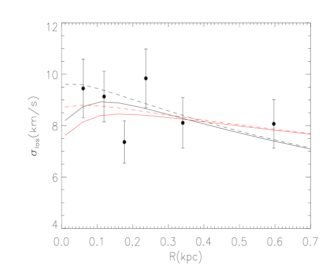
Figure 1: The line-of-sight star velocity dispersion as a function of the projected radius for Draco. Observations were taken from [68]. The solid and dotted lines are fits from our halo model, see text for details.

To compute $\sigma_{los}$ for our halo model, we follow the formulas described in [69] and [70]. Of most importance is the use of the integral formula for the line-of-sight velocity dispersion presented in the appendix of [70] (isotropic case, $B=0$):

$$\sigma^{2}_{los}(R)=\frac{\Gamma(2m)}{\Gamma((3-p)m)}\frac{r_{v}}{a_{s}}V_{v}^{2}\textrm{exp}(X^{1/m})\int_{X}^{\infty}\sqrt{1-\left(\frac{X}{x}\right)^{2}}\tilde{\ell}(x)\tilde{M}(x)\frac{dx}{x}$$ (17)

where $\tilde{\ell}(x)=x^{-p}\textrm{exp}(-x^{1/m})$ is the dimensionless 3D luminosity density of the stellar component (which can be obtained by deprojecting the surface brightness profile, modeled in [69] by a Sérsic law), $p=1-0.6097/m+0.05463/m^{2}$; $\tilde{M}(x)=\tilde{M}_{DM}(x)+f_{\star}\tilde{M}_{\star}(x)$ is the dimensionless mass profile consisting of dark matter, $\tilde{M}_{DM}$, and stellar, $\tilde{M}_{\star}$, components; $a_{s}$ and $m$ are the free parameters of the Sérsic profile, and finally $x=r/a_{s}$, $X=R/a_{s}$. Eq. (17) is generically valid for any halo model with spherical symmetry. The stellar component has 3 parameters: $a_{s}$, $m$ and $f_{\star}$, the first two are constrained by the brightness profile of Draco [71]: $a_{s}=7.3$ arcmin ($\sim 0.17$ kpc for a distance to Draco of 80 kpc) and $m=0.83$. And $f_{\star}=M_{\star}/M_{v}$, where $M_{\star}=6.6\times 10^{5}M_{\odot}$ ([69]).

Using Eq. (17) together with our halo model, we can find fits to the observational data using 2 free parameters: $M_{v}$ and $\rho_{c}$, and using the central value for the concentration parameter (Eq. (11)) altogether with its expected dispersion $\sigma_{logc}\approx 0.095$. In Fig. (1) we show different fits to the observational data, the black (thicker) and red (thinner) lines are for the upper and lower values of the concentration parameter respectively. We found that for the lower values of the concentration parameter, red (thinner) lines, the best fit to the data is a model which converges towards a halo with no core (red (thinner) dashed line). Increasing the core radius reduces the goodness of the fit, we measured this evaluating $\chi^{2}/df$, where $df$ is the number of degrees of freedom: number of data points - number of parameters. On the contrary, for higher values of the concentration parameter, black (thicker) lines, the best fit is found for a model with core (black (thicker) solid line), the goodness of the fit is statistically reduced with decreasing core radii, the convergence to a halo with no core is shown as a dashed black (thicker) line. These results imply that our model with high values of the concentration parameter is able to give an adequate description of the actual observations for Draco.

Our whole model is built on the assumption of a model with core, this goes back to Eqs. (4) and (3), so we should clearly concentrate on the fits corresponding to a model with a core. In the search for the best fit to $\sigma_{los}$, this can be done unambiguously only for certain values of the concentration (those on the high end of the expected concentration interval). For instance, the red (thinner) solid line is as good fit to the observational data as the black (thicker) solid line, however, we can not extract the value of $\alpha$ without ambiguity for the latter since reducing the core radius increases the goodness of the fit, recall that convergence is reached for $r_{c}\rightarrow 0$ kpc. The core model which we find to be a good fit to the observational data (black (thicker) solid line) has the following parameters: $M_{v}=1.5\times 10^{9}M_{\odot}$, $\rho_{c}=3.1\times 10^{8}M_{\odot}$kpc³, $r_{c}=0.11$kpc, $r_{v}=30$kpc, $c=26.6$ and $\alpha=28.7$.

We believe that this value of $\alpha$ for Draco is reasonable and certainly consistent with the interval obtained before (Eq. (16)). As a complementary check, we have used another set of data on the velocity dispersion of Draco ([72]) to fit our model. Although larger values for the virial mass and core radius are needed to achieve a good fit, we found the value of $\alpha$ to be consistent with the interval of values given in (Eq. (16). Nevertheless it should be stressed that better observational constraints are needed to put firmer constraints on the value of $\alpha$, which is particularly sensitive to the value of $\rho_{c}$ ($r_{c}$). The value of $\alpha$ is of course also sensitive to the chain of assumptions needed to arrive to its final estimate, concentration values have an important role as can be seen on figure 1. The assumption of isotropic velocity dispersion, B=0 in Eq. (14), has also an influence in the values found for the model parameters in the fit to Draco. The addition of anisotropy to our model would alter the values of the best fit parameters found for Draco, and therefore the value of $\alpha$ we just reported. The impact of anisotropy on the value of $\alpha$ can only be properly quantified by improving our model with the removal of the restriction B=0, and redoing the analysis we have made so far. Such task is left as a possible future work once further more precise constraints on the dynamical properties of dark matter dominated systems like Draco are available. We believe that the assumption of isotropy is sufficient for the purposes of this work to calculate approximately the value of $\alpha$.

Overall, taking into account all the assumptions we have made to fit our model with observational data, we consider that the interval of values obtained for the “ignorance parameter” $\alpha$, do give a reasonably description to the several galactic samples for which we have tested our model, thus making us feel confident on the overall entropy criteria presented in this work, at least as a first order indirect analysis of real dark matter structures.

5 Analysis of the mSUGRA parameter space

Supersymmetry has attracted attention since it was first proposed for its many intriguing theoretical features and also for providing an elegant solution to the hierarchy problem (for an excellent introduction to the supersymmetry formalism and phenomenology see [3]).

The minimal phenomenologically viable supersymmetric extension of the SM is called the Minimal Supersymmetric Standard Model (MSSM). The MSSM has appealing features: it is in much better agreement with the assumption of unification of the gauge couplings than the Standard Model [21], besides, it provides with a good dark matter candidate when the lightest supersymmetric particle (LSP) is the neutralino (see for instance [22]). In the MSSM every known particle is associated to a superpartner to form either a chiral or a gauge supermultiplet, whose spin components differ from each other by $1/2$. In addition it has two $SU(2)$ doublet complex scalar Higgs fields ($H_{u}$ and $H_{d}$) in order to give masses to the up and down type particles and to avoid gauge anomalies. The ratio of the vacuum expectation values of the neutral part of these two Higgs doublets is known as $\tan\beta=<H^{0}_{u}>/<H^{0}_{d}>=v_{u}/v_{d}$. The MSSM includes a discrete matter parity called R parity. All the SM particles have charge $+1$ under this symmetry, whereas the supersymmetric partners have charge $-1$. R parity is responsible for the stability of the LSP.

Since we do not observe any of the superpartners at the current laboratory energies, if supersymmetry exists it has to be broken. The breaking of SUSY introduces around $\sim 100$ new parameters, called soft breaking SUSY terms. These are constrained by the limits on flavour changing neutral currents and CP-violating processes, which lead to the assumption of “universality” of the soft breaking terms. The universality condition means that the gaugino masses have a common value at the GUT scale, and the same assumption is made for the scalar (squark and sleptons) masses and the trilinear couplings respectively. After SUSY and electroweak symmetry breaking, there is mixing between different squarks, sleptons, and Higgses with the same electric charge, and between the gauginos and electroweak Higgsinos. Thus, the low energy mass spectrum of the MSSM contains the usual SM particles, squarks and sleptons, four neutralinos (denoted by $\chi_{1,2,3,4}^{0}$), two charginos ($\chi^{\pm}_{1,2}$), the gluino, and five Higgs bosons: the usual light SM-like Higgs $M_{Higgs}$, a heavy neutral one $M_{H}$, two charged ones $M_{H}^{\pm}$, and a pseudoscalar $M_{A}$.

Minimal supergravity (mSUGRA) is one of the better studied SUSY breaking scenarios [23]. In this class of models supersymmetry is broken spontaneously in a hidden sector that connects only through gravitational-strength interactions with the MSSM or visible sector. In the visible sector these interactions induce the appearance of the soft SUSY breaking terms. These are determined by only five parameters, a universal mass for the gauginos at the GUT scale $m_{1/2}$, a universal mass for the scalars $m_{0}$, a universal trilinear coupling $A_{0}$, $\tan\beta$, and the sign of the Higgsino mass parameter $\mu$. This drastic reduction in the number of parameters facilitates the scanning of interesting regions of the parameter space. This is usually done by fixing two parameters, for instance $A_{0}$ and $\tan\beta$. It is also possible to vary the four continuous parameters freely using Monte Carlo techniques with interesting results [24, 25].

We are finally in a position to use both the abundance and entropy criteria, to compute the total mass density of neutralinos today, and constrain the region in the mSUGRA parameter space where both criteria are fulfilled. Out of the five parameters of the model, we will consider that the Higgsino mass parameter has a positive sign. This consideration is based on studies of the anomalous magnetic moment of the muon $g_{\mu}-2$, where SUSY models with a positive sign of $\mu$ can give a much better agreement with the experimental value of $g_{\mu}-2$ than in the Standard Model, whereas negative values do not solve this problem [26]-[29].

Our strategy is then to explore broad regions of values for the other four parameters, by means of a bidimensional analysis in the $m_{0}-m_{1/2}$ plane with different fixed values of $A_{0}$ and tan$\beta$. It is important to mention that we are not presenting an exhaustive search in all the possible regions, but we concentrate on those regions which have received more attention in the literature, see for example [4].

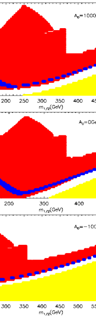
Figure 2: Allowed regions in the parameter space for AC (lighter gray, red) and EC (darker grey, blue) for the mSUGRA model with sgn$\mu=+$, tan$\beta=10$, and $A_{0}=1000$ GeV, top panel, $A_{0}=0$ GeV, middle panel, and $A_{0}=-1000$ GeV, bottom panel. The yellow region (lower right corner) is where the $\tilde{\tau}$ is the LSP. The figure shows the so called bulk and coannihilation regions.

In Fig. (2), we present the results for tan$\beta=10$, and for three values of $A_{0}$, namely $A_{0}=1000,0,-1000$ GeV, shown in the top, middle and bottom panels respectively. The figure shows the so called bulk and coannihilation regions. The yellow region (lower right corner) is where the stau $\tilde{\tau}$ is the LSP, the lighter and darker areas (red and blue for the online version in colors) define the allowed regions for the EC and AC respectively according to the observed value of $\Omega_{DM}$. The area of the EC region depends on the size of the interval of values of the parameter $\alpha$, Eq.(16), the lower and upper bounds of $\alpha$ determine the upper and lower boundaries of the EC region. As can be seen from the figure, the region where both criteria are fulfilled is very small, in fact, only for the highest values of $\alpha$ there is an intersection between both criteria. This behavior holds for all values of $A_{0}$ in the interval $[-1000,1000]$ GeV; here we are showing the results only for the extreme and central values of $A_{0}$.

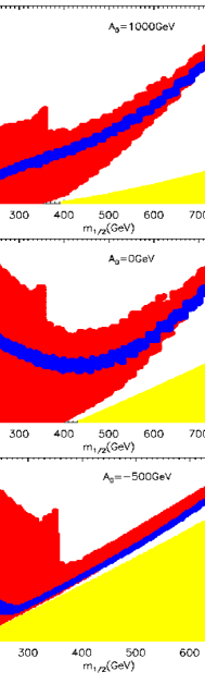
Figure 3: The same as Fig. (2), but for tan$\beta=50$, and now $A_{0}=-500$ GeV in the bottom panel.

Repeating the same procedure for larger values of tan$\beta$, we find that the intersection region for both criteria becomes larger, getting more significant for larger values of this parameter. This is clearly shown in Fig. (3), equivalent to Fig. (2), but for tan$\beta=50$. In this case the bottom panel is for $A_{0}=-500$ GeV. It is clear from the figure that for this value of tan$\beta$, both criteria are consistent, there is a large intersection area for values of $A_{0}$ in the interval $[0,1000]$ GeV. For negative values of $A_{0}$, the intersection region decreases as $A_{0}$ does so, see the bottom panel of Fig. (3). For even lower values of $A_{0}$ the intersection becomes insignificant.

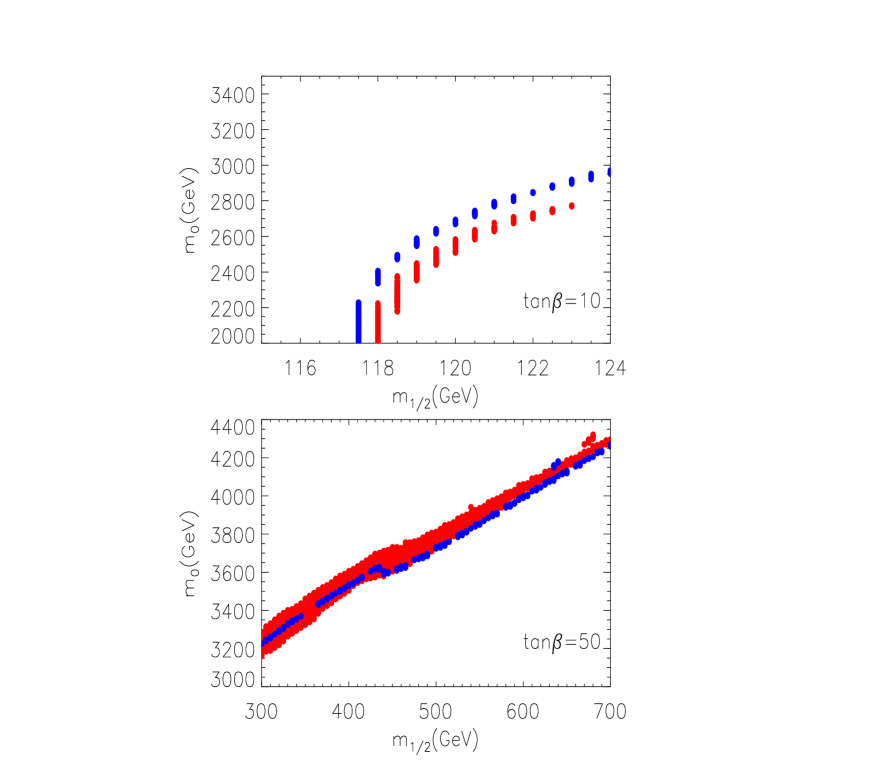
Figure 4: Allowed regions in the parameter space for AC (lighter gray, red) and EC (darker grey, blue) in the mSUGRA model with $A_{0}=0$, sgn$\mu=+$, tan$\beta=10$, top panel, and tan$\beta=50$, bottom panel. The figure shows the so called Focus Point region.

In Fig. (4) we present the same analysis but for a different region of the parameter space (high values of $m_{0}$), known as Focus Point region, and for the central value $A_{0}=0$. The situation is consistent with the previous result, both criteria intersect for $\tan\beta=50$ and there is no intersection for $\tan\beta=10$.

This analysis allows us to arrive to one of the main results of our work. The use of both criteria favors large values of tan$\beta$.

It is interesting to point out that, within the AC formulation, the dark matter density constraint reduces effectively the allowed regions in the mSUGRA parameter space to strips pointing to an almost linear trend between $m_{0}$ and $m_{1/2}$, at least in the coannihilation and focus point regions, as can be clearly seen in the darker (blue) areas in Figs. (2, 3, 4). This type of behavior has been noticed previously in [30], where the authors even give some parameterizations for these so called “WMAP lines”. Notice that this type of relation is also shown within the EC description in the above mentioned regions, although the “WMAP lines” are not as narrow as in the AC formulation, because of the wide range in the $\alpha$ parameter Eq. (16). A deeper analysis of the connections among the mSUGRA parameters could reveal the original cause for such behavior, shown in both, quite independent, criteria.

The regions that were compatible with the abundance and entropy criteria were analyzed to see what restrictions they imposed on the SUSY spectra. This was done just in order to show the expected mass spectra resulting from these constraints. The analysis was performed using micrOMEGAs linked to Suspect [11], using the default input values of micrOMEGAs, for instance:

$$M_{\rm top} = 175\,{\rm GeV},$$ (18)

$$m_{\rm bot} = 4.23\,{\rm GeV}.$$ (19)

The Higgs bosons masses, as well as the rest of the superpartner masses, depend directly on the Universal gaugino mass $m_{1/2}$ and the Universal scalar mass $m_{0}$. The first noticeable fact is that the bound on the Higgs mass [31]:

$$m_{\rm Higgs}\geq 114\,{\rm GeV,}$$ (20)

favors the results with large $\tan\beta$ for the bulk and co-annihilation regions, as can be seen from Fig. (5), which shows the Higgs mass $M_{Higgs}$ plotted against the mass of the LSP. In the case of both the bulk and co-annihilation regions, for $\tan\beta=10$ only a small region of parameter space is allowed, with $m_{\chi}\sim 160$ GeV. In this same case for $\tan\beta=50$ the allowed SUSY spectra starts for $m_{\chi}\geq 141$ GeV. In the case of the focus point region the Higgs mass does not impose any further constraint, and $m_{\chi}\geq 114$ GeV.

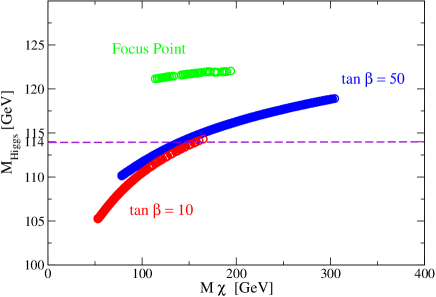
Figure 5: The figure shows the Higgs mass plotted versus the LSP mass. Points above the dashed line are the allowed values for the LSP.

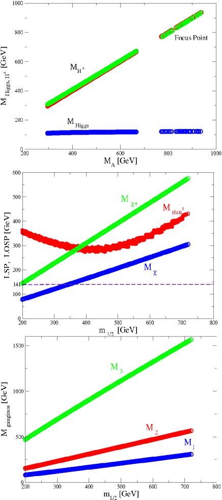
Figure 6: The lightest $M_{Higgs}$ and heavier Higgs bosons $M_{H},~{}M_{H}^{+}$ plotted against $M_{A}$ for $\tan\beta=50$ (top panel). The lines to the right of the graph correspond to the focus point region, where the masses are in general heavier (except for $M_{Higgs}$). The mass of the LOSP plotted against $m_{1/2}$ for $\tan\beta=50$ in the bulk and co-annihilation regions (middle panel). The masses of the gauginos $M_{1},~{}M_{2},~{}M_{3}$ plotted against $m_{1/2}$ for $\tan\beta=50$ also in the bulk and co-annihilation regions (bottom panel).

Fig. (6) top panel, shows the different Higgs bosons masses plotted against the pseudoscalar one $M_{A}$, for $\tan\beta=50$. As can be seen from the graph, the heavy neutral $M_{H}$ and charged $M_{H^{+}}$ Higgs bosons are much heavier than the lightest one, and almost degenerate in mass. The lightest supersymmetric observable particle LOSP is plotted against $m_{1/2}$ for $\tan\beta=50$ for the bulk and co-annihilation regions. The region above the dashed line shows the allowed values after the constraint on $M_{Higgs}$ is taken into account. A comparison of the LSP with the LOSP shows that for this region, for smaller values of $m_{1/2}$ the LOSP will be the lightest chargino $\chi^{\pm}$ (which is practically degenerate in mass to the second lightest neutralino), and very close in mass with the stau. As $m_{1/2}$ increases the LOSP is the stau, again with values very close to the LSP, as expected. For the focus point region the LOSP is the lightest chargino $\chi_{1}^{\pm}$, followed by the second neutralino $\chi^{0}_{2}$, with almost degenerate masses. Similar results hold for $\tan\beta=10$ albeit for a much more reduced region in parameter space. The gauginos $M_{1},~{}M_{2},~{}M_{3}$ are plotted against $m_{1/2}$ in the bottom panel for $\tan\beta=50$. The masses of these particles on the focus point region are very similar to the ones shown in the figure (they basically lie along the same lines). In both, large and small $\tan\beta$ cases, the gluino is much heavier than the other two gauginos, as expected, and this difference increases with a larger value of the neutralino mass, or equivalently, with larger $m_{1/2}$.

6 Conclusions

We have followed the novel idea of [7] to introduce a new criterion to constrain the mSUGRA parameter space, which uses the assumption of entropy consistency for the initial and final states of a neutralino gas. Using the program micrOMEGAs, we explored with precision which regions simultaneously satisfy this criterion and the usual abundance criterion previously used in the literature.

Combining both, and using one of the most recent analysis that combines observations coming from different sources to constrain the actual dark matter density, we were able to show that both criteria are compatible for large values of $\tan\beta$, in particular for tan$\beta=50$, and that for lower values ($\tan\beta=10$), the coincidence is scarce. The result then favors the scenario where the ratio of the vacuum expectation values for the neutral supersymmetric Higgs bosons is large. Some other SUSY extensions of the SM, taken together with LEP data [32], can also favor large values of $\tan\beta$ (for instance Grand Unified or supergravity models with Yukawa coupling unification (see for instance [33, 34]), or Finite Unified Theories (see for instance [35, 36])).

Moreover, we went a step further and analyze the mass spectrum of the SUSY particles and obtained a bound for the neutralino mass for the bulk and co-annihilation region, $m_{\chi}\geq 141$ GeV, which is higher than the actual experimental constraint, $m_{\chi}>46$ Gev [37].

In the process to obtain the presented results, we described carefully a method to obtain an empirical interval on the values for $\alpha$, a parameter reflecting the present ignorance on the appropriate statistical-mechanics description on dark matter systems. We used a halo model with a constant density core in the center followed by an NFW profile to describe dark matter dominated systems, which are the astrophysical systems for which our model is suitable. We found that, although $\alpha$ is a model dependent quantity, the bounds reported in this paper for its value (Eq. (16)) are reliable, considering the different range of observational data we used to constrain its value. More precise observations on the line-of-sight velocity dispersion of dwarf spheroidals are promising to improve our results.

Finally, we want to remark that the analysis presented in this work is robust and it can be done for any other particle claimed to be candidate for dark matter, or for other supersymmetric extensions of the Standard Model. Also, our results can be extended for other regions of the parameter space, for instance, analyzing $A_{0}\neq 0$ for the Focus Point region, $\mu<0$ and exploring the “rapid annihilation funnel” region (see for example right panel, Fig. (4) of [38]).

References

References

-
[1]
Bennett C L et al. (The WMAP collaboration), First-Year Wilkinson Microwave Anisotropy
Probe (WMAP) Observations: Preliminary Maps and Basic Results, 2003 Astrophys. J. S. S. 148 1
[astro-ph/0302207]
See also Spergel D N et al (The WMAP collaboration), First-Year Wilkinson Microwave Anisotropy Probe (WMAP) Observations: Determination of Cosmological Parameters, 2003 Astrophys. J. S. S. 148 175 [astro-ph/0302209];
Spergel D N et al. (The WMAP collaboration), Three-Year Wilkinson Microwave Anisotropy Probe (WMAP) Observations: Implications for Cosmology, 2007 Astrophys. J. S. S. 170 377 [astro-ph/0603449] - [2] Seljak U, Slosar A and McDonald P, Cosmological parameters from combining the Lyman- forest with CMB, galaxy clustering and SN constraints, 2006 J. Cosm. Astropart. Phyis. 10 014 [astro-ph/0604335]
- [3] M. F. Sohnius, Phys. Rept. 128 (1985) 39; Martin S P,A Supersymmetry Primer, 1998 Perspectives on Supersymmetry. Advanced Series on Directions in High Energy Physics. Edited by Gordon L. Kane. Published by World Scientific Publishing Company, Singapore 18 1 [hep-ph/9709356]
- [4] Bélanger G, Kraml S and Pukhov A, Comparison of supersymmetric spectrum calculations and impact on the relic density constraints from WMAP, 2005 Phys. Rev. D 72 015003 [hep-ph/0502079]
- [5] Bélanger G, Boudjema A, Pukhov A, and Semenov, A, WMAP constraints on SUGRA models with non-universal gaugino masses and prospects for direct detection, 2005 Nucl. Phys. B 706 411 [hep-ph/0407218]
- [6] Bélanger G, Boudjema A, Pukhov A, and Semenov, A, micrOMEGAs: Version 1.3, 2006 Comput. Phys. Commun. 174 577 [hep-ph/0405253]
- [7] Cabral-Rosetti L G, Hernández X and Sussman R A, Using entropy to discriminate annihilation channels in neutralinos making up galactic halos, 2004 Phys. Rev. D 69 123006
- [8] Nunez D, Sussman R A, Zavala J, Nellen L, Cabral-Rosetti L G and Mondragon, M, Entropy considerations in constraining the mSUGRA parameter space, 2006 10th Mexican Workshop on Particles and Fields, Morelia, Mexico, AIP Conference Proceedings 2005 857 321 [astro-ph/0604127]
- [9] Jungman G, Kamionkowski M and Griest K, Supersymmetric dark matter, 1996 Phys. Rept. 267 195 [hep-ph/9506380]
- [10] Gondolo P and Gelmini G, Cosmic abundances of stable particles: Improved analysis, 1991 Nucl. Phys. B 360 145
- [11] Djouadi A, Kneur J L and Moultaka G, SuSpect: A Fortran code for the Supersymmetric and Higgs particle spectrum in the MSSM, 2007 Comput. Phys. Commun. 176 426 [hep-ph/0211331]
- [12] Tsallis C, Nonextensive statistics: Theoretical, experimental and computational evidences and connections, 1999 Braz J Phys 29 1 [cond-mat/9903356]
- [13] Nunez D, Sussman R A, Zavala J, Cabral-Rosetti L G and Matos T, Empirical testing of Tsallis’ Thermodynamics as a model for dark matter halos, 2006 10th Mexican Workshop on Particles and Fields, Morelia, Mexico, AIP Conference Proceedings 2005 857 316 [astro-ph/0604126]
- [14] Zavala J, Nunez D, Sussman R A., Cabral-Rosetti L G and Matos T, Stellar polytropes and Navarro Frenk White halo models: comparison with observations, 2006 J. Cosm. Astropart. Phys. 06 008 [astro-ph/0605665]
- [15] Pathria R K, Statistical Mechanics, 1972 (Pergamon Press)
- [16] Binney J and Tremaine S, Galactic Dynamics, 1987 (Princeton University Press
- [17] Padmanabhan T, Theoretical Astrophysics, Volume I: Astrophysical Processes, 2000 (Cambridge University Press)
- [18] Katz J, Horwitz G and Dekel A, Steepest descent technique and stellar equilibrium statistical mechanics. IV - Gravitating systems with an energy cutoff, 1978 Astrophys. J. 223 299
- [19] Katz J, Stability limits for ’isothermal’ cores in globular clusters, 1980 Mon. Not. R. Astron. Soc. 190 497
- [20] Magliocchetti M, Pugacco G and Vesperini E, Gravothermal catastrophe in anisotropic systems, 1997 Nuovo Cimento B 112 423 [astro-ph/9806233]
- [21] U. Amaldi, W. de Boer, and H. Furstenau, Phys. Lett. B 260, 447 (1991); C. Giunti, C.W. Kim and U.W. Lee, Mod. Phys. Lett. A 6, 1745 (1991);
- [22] G. Jungman, M. Kamionkowski and K. Griest, Phys. Rept. 267 (1996) 195 [arXiv:hep-ph/9506380].
- [23] H. P. Nilles, Phys. Rept. 110 (1984) 1.
- [24] E. A. Baltz and P. Gondolo, JHEP 0410 (2004) 052 [arXiv:hep-ph/0407039].
- [25] B. C. Allanach and C. G. Lester, Phys. Rev. D 73 (2006) 015013 [arXiv:hep-ph/0507283].
- [26] Bennett G et al., Final report of the E821 muon anomalous magnetic moment measurement at BNL, 2006 Phys. Rev. D 73 072003 [hep-ex/0602035]
- [27] Davier M, The Hadronic Contribution to g, 2007 Nucl. Phys. B Proceedings S. 169 288 [hep-ph/0701163]
- [28] Moroi T, Muon anomalous magnetic dipole moment in the minimal supersymmetric standard model, 1996 Phys. Rev. D 53 6565 [hep-ph/9512396] See also Moroi T, Erratum: Muon anomalous magnetic dipole moment in the minimal supersymmetric standard model [Phys. Rev. D 53, 6565 (1996)], 1997 Phys. Rev. D 56 4424
- [29] Heinemeyer S, Stöckinger D and Weiglein G, Electroweak and supersymmetric two-loop corrections to , 2004 Nucl. Phys. B 699 103 [hep-ph/0405255]
- [30] Battaglia M, Roeck A D, Ellis J, Gianotti F, Olive K A and Pape L, Updated post-WMAP benchmarks for supersymmetry 2004 European Physical J. C 33 273 [hep-ph/0306219]
- [31] ALEPH Collaboration, DELPHI Collaboration, L3 Collaboration, OPAL Collaboration and The LEP Working Group For Higgs Boson Searches, Search for the Standard Model Higgs boson at LEP 2003 Phys. Lett. B 565 61 [hep-ex/0306033]
- [32] ALEPH Collaboration, DELPHI Collaboration, L3 Collaboration, OPAL Collaboration and the LEP Higgs Working Group, Searches for the Neutral Higgs Bosons of the MSSM: Preliminary Combined Results Using LEP Data Collected at Energies up to 209 GeV 2001 Submitted to EPS’01 in Budapest and Lepton-Photon ’01 in Rome [hep-ex/0107030]
- [33] Olechowski M and Pokorski S, Hierarchy of quark masses in the isotopic doublets in N=1 supergravity models 1988 Pjys. Lett. B 214 393
- [34] Ananthanarayan B, Lazarides G and Shafi Q, Radiative electroweak breaking and sparticle spectroscopy with tan 1993 Phys. Lett. B 300 245
- [35] Djouadi A, Heinemeyer S, Mondragon M and Zoupanos G, Finite Unified Theories and the Higgs Mass Prediction 2004 Springer Proceedings in Physics 98 273 [hep-ph/0404208]
- [36] Kapetanakis D, Mondragon M and Zoupanos G, Finite unified models 1993 Zeitschrift für Physik C Particles and Fields 60 181 [hep-ph/9210218]
- [37] Yao W M et al. (Particle Data Group), Review of Particle Physics 2006 J. Phys. G 33 1 [astro-ph/0601514]
- [38] Feng J L, Dark matter at the Fermi scale 2006, Journal of Physics G: Nuclear and Particle Physics 32 R1 [astro-ph/0511043]
- [39] CDMS collaboration, A Search for WIMPs with the First Five-Tower Data from CDMS 2008 [arXiv:0802.3530]
- [40] Eke V R, Navarro J F and Frenk C S, The Evolution of X-Ray Clusters in a Low-Density Universe 1998 Astrophys. J. 503 569 [astro-ph/9708070]
- [41] Faltenbacher A, Hoffman Y, Gtlober S and Yepes G, Entropy of gas and dark matter in galaxy clusters 2007 Mon. Not. R. Astron. Soc. 376 1327 [astro-ph/0608304]
- [42] Navarro J F, Frenk C S and White S D M, A Universal Density Profile from Hierarchical Clustering 1997 Astrophys. J. 490 493 [astro-ph/9611107]
- [43] Natarajan P, Croton, D and Bertone G, Consequences of dark matter self-annihilation for galaxy formation 2007 [arXiv:0711.2302]
- [44] Mo H J, Mao S and White S D M, The formation of galactic discs 1998 Mon. Not. R. Astron. Soc. 295 319 [astro-ph/9707093]
- [45] Lokas E L and Mamon G A, Properties of spherical galaxies and clusters with an NFW density profile 2001 Mon. Not. R. Astron. Soc. 321 155 [astro-ph/0002395]
- [46] Lokas E L and Hoffman Y, Nonlinear evolution of spherical perturbation in a non-flat Universe with cosmological constant 2001 [astro-ph/0108283]
- [47] Lokas E L, Structure Formation in the Quintessential Universe 2001 Acta Phys. Pol. B 32 3643
- [48] Neto A F, Gao L, Bett P, Cole S, Navarro J F, Frenk C S, White S D M, Springel V and Jenkins A, The statistics of CDM halo concentrations 2007 Mon. Not. R. Astron. Soc. 381 1450
- [49] Springel V et al., Simulations of the formation, evolution and clustering of galaxies and quasars 2005 Nature 435 629
- [50] Zavala J, Avila-Reese V, Hernández-Toledo H and Firmani C, The luminous and dark matter content of disk galaxies 2003 Astron. Astrophys. 412 633 [astro-ph/0305516]
- [51] de Blok W J G, McGaugh S S and Rubin V C, High-Resolution Rotation Curves of Low Surface Brightness Galaxies. II. Mass Models 2001 Astron. J. 122 2396
- [52] de Blok W J G, McGaugh S S, Bosma A and Rubin V C, Mass Density Profiles of Low Surface Brightness Galaxies 2001 Astrophys. J. 552 23 [astro-ph/0103102]
- [53] Binney J J and Evans N W, Cuspy dark matter haloes and the Galaxy 2001 Mon. Not. R. Astron. Soc. 327 L27 [astro-ph/0108505]
- [54] Borriello A and Salucci P, The dark matter distribution in disc galaxies 2001 Mon. Not. R. Astron. Soc. 323 285 [astro-ph/0001082]
- [55] Blais-Ouellette S, Carignan C and Amram P, Multiwavelength Rotation Curves to Test Dark Halo Central Shapes 2002 ASP Conference Proceedings 282 129 [astro-ph/0203146]
- [56] Bosma A, Dark Matter in Galaxies: Observational overview 2004 IAU Symposium 220, Sydney, Australia. Eds: S. D. Ryder, D. J. Pisano, M. A. Walker, and K. C. Freeman. San Francisco: Astronomical Society of the Pacific., p.39 [astro-ph/0312154]
- [57] Pointecouteau E, Arnaud M and Pratt G W, The structural and scaling properties of nearby galaxy clusters. I. The universal mass profile 2005 Astron. Astrophys. 435 1 [astro-ph/0501635]
- [58] Voigt L M and Fabian A C, Galaxy cluster mass profiles 2006 Mon. Not. R. Astron. Soc. 368 518 [astro-ph/0602373]
- [59] Zappacosta L, Buote D A, Gastaldello F, Humphrey P J, Bullock J, Brighenti F and Mathews W, The Absence of Adiabatic Contraction of the Radial Dark Matter Profile in the Galaxy Cluster A2589 2006 Astrophys. J. 650 777 [astro-ph/0602613]
- [60] Navarro J F, Hayashi E, Power C, Jenkins A R, Frenk C S, White S D M, Springel V, Stadel J and Quinn T R, The inner structure of CDM haloes - III. Universality and asymptotic slopes 2004, Mon. Not. R. Astron. Soc. 349 1039 [astro-ph/0311231]
- [61] Diemand J, Zemp M, Moore B, Stadel J, Carollo C M, Cusps in cold dark matter haloes 2005, Mon. Not. R. Astron. Soc. 364 665 [astro-ph/0504215]
- [62] Matos T, Nunez D and Sussman R A, A general relativistic approach to the Navarro Frenk White galactic halos 2004 Class. Quantum Grav. 21 5275 [astro-ph/0410215]
- [63] Dehnen W and McLaughlin D, Dynamical insight into dark matter haloes 2005 Mon. Not. R. Astron. Soc. 363 1057 [astro-ph/0506528]
- [64] Hansen S H and Moore B, A universal density slope Velocity anisotropy relation for relaxed structures 2006 New Astron. 11 333
- [65] Kuzio de Naray R, McGaugh S S, de Blok W J G and Bosma A, High-Resolution Optical Velocity Fields of 11 Low Surface Brightness Galaxies 2006 Astrophys. J. S. S. 165 461 [astro-ph/0604576]
- [66] Firmani C, D’Onghia E, Chincarini G, Hernández X and Avila-Reese V, Constraints on dark matter physics from dwarf galaxies through galaxy cluster haloes 2001 Mon. Not. R. Astron. Soc. 321 713 [astro-ph/0005001]
- [67] Wilkinson M I, Kleyna J T, Evans N W, Gilmore G F, Irwin M J and Grebel E K, Kinematically Cold Populations at Large Radii in the Draco and Ursa Minor Dwarf Spheroidal Galaxies 2004 Astrophys. J. 611 L21
- [68] Sánchez-Conde M A, Prada F, Lokas E L, Gómez M E, Wojtak R and Moles M, Dark matter annihilation in Draco: New considerations of the expected gamma flux 2007 Phys. Rev. D 76 123509 [astro-ph/0701426]
- [69] Lokas E L, Mamon G A and Prada F, Dark matter distribution in the Draco dwarf from velocity moments 2005 Mon. Not. R. Astron. Soc. 363 918
- [70] Mamon G A and Lokas E L, Dark matter in elliptical galaxies - II. Estimating the mass within the virial radius 2005 Mon. Not. R. Astron. Soc. 363 705
- [71] Odenkirchen M et al., New Insights on the Draco Dwarf Spheroidal Galaxy from the Sloan Digital Sky Survey: A Larger Radius and No Tidal Tails 2001 Astrophys. J. 122 2538
- [72] Walker M G, Mateo M, Olszewski E W, Gnedin O Y, Wang X, Sen B and Woodroofe M, Velocity Dispersion Profiles of Seven Dwarf Spheroidal Galaxies 2007 Astrophys. J. L. 667 L53