A quantum decay model with exact explicit analytical solution

Abstract

A simple decay model is introduced. The model comprises of a point potential well, which experiences an abrupt change. Due to the temporal variation the initial quantum state can either escape from the well or stay localized as a new bound state. The model allows for an exact analytical solution while having the necessary features of a decay process. The results show that the decay is never exponential, as classical dynamics predicts. Moreover, at short times the decay has a fractional power law, which differs from perturbation quantum methods predictions.

Despite the fact that almost all the decay processes in nature observed of having an exponential decay law, it is well known that quantum mechanics predicts deviation from this law Fondaetal_1 ; Greenland_2 ; Chiuetal_3 .

In fact, it has been proven by Khalfin Khalfin_4 that the long time behavior of the non-decay probability cannot be exponential, and in practical cases it has a negative power decay law. Moreover, at short times most quantum systems obey $t^{2}$ dependence. This kind of dependence is usually attributed to a reversible process, which contradicts an irreversible decay to the continuum.

Recently, it became technologically feasible to measure this deviation from exponential law, and indeed it was demonstrated experimentally Menonetal_5 ; Wilkinsonetal_6 ; Grenland_7 .

The scenario of an irreversible decay of a confined bound state to the continuum is ubiquitous in the physical world, Beta decay is such a realization. Hence, resolving this controversy is required to the understanding of these basic processes. Theoretically, this problem was confronted by applying an abrupt perturbation on the initial confined state. However, this perturbation approach merely emphasizes the controversy except for the intermediate times where an approximately exponential law seems to appear CohenTannoudjietal_8 . At short times the reminiscent of a reversible $t^{2}$ law is still dominant.

The recent technological developments, which allow trapping cold atoms in very small traps Szriftgiseretal_9 ; Fortetal_10 , also allow to release them almost instantaneously (since the trapping is done by laser beams). As a consequence, the temporal dynamics and decay of quantum particles at the presence of an abruptly changing potential can also be investigated in the laboratory. In this paper we investigate a simple quantum mechanical model, which can emulate realistic decay scenarios. The initial state is a bound eigenstate of a localized potential well, and the model allows investigating the state dynamics due to abrupt change in this potential well. To simplify the model we use a delta-function potential well. It is well known that this kind of a potential can emulate any barrier/well whose de-Broglie wavelength is considerably longer than the potential physical dimensions Granot_11 . In other words, for most practical purposes it can replace any point potential. On the other hand, a point potential brings in singularity to the system and as a result a fractional power law emerges. However, as was mentioned elsewhere GranotMarchewka_12 some reminders to this behavior can be traced even in the analytic potential case.

The main strength of this model is that it has an exact analytical solution and no approximations are taken. We show that the dynamics of this model does not look exponential at any time. Moreover, at short times (as well as at very long times) the dynamics is governed by a fractional power law instead of an integral power law. To the best of our knowledge, this is the only quantum decay model, where the final state can be either localized or extended, and has an exact analytical solution.

We use a delta function to simulate the attractive potential well

$$V\left({x,t}\right)=\left\{{{\begin{array}[]{*{20}c}{-2\alpha\delta\left(x\right)\hfill}&{\mbox{for}\hfill}&{t\leq 0\hfill}\\ {-2\lambda\delta\left(x\right)\hfill}&{\mbox{for}\hfill}&{t>0\hfill}\\ \end{array}}}\right.$$ (1)

That is, the potential can be written as an initial stationary potential $V_{0}\left(x\right)=-2\alpha\delta\left(x\right)$ and a perturbation part $\Delta V\left({x,t}\right)=2\left({\alpha-\lambda}\right)u\left(t\right)\delta\left(x\right)$ [$u\left(x\right)$ is the heaviside function $u\left(x\right)=\left\{{\mbox{0 for }x<0\mbox{; 1 for }x>0}\right\}$]. The Schrödinger equation reads

$$i\frac{\partial\psi}{\partial t}=-\frac{\partial^{2}\psi}{\partial x^{2}}+V_{0}\left(x\right)\psi+\Delta V\left({x,t}\right)\psi$$ (2)

hereinafter we adopt the units $\hbar=1$ (Planck constant) and $2m=1$(particle mass). It should be stressed that any shallow potential well ($\Delta x>>\left({U_{0}}\right)^{-1/2}$with width $\Delta x$ and depth $-U_{0})$ can be replaced, for most practical purposes, by a delta function potential $V_{initial}\left(x\right)=-2\alpha\delta\left(x\right)$ with the prefactor $2\alpha=U_{0}\Delta x$, since the two scatterers have a very similar scattering and a single bound state ( for a positive potential see, for example Granot_11 ).

By applying the same analysis and logic of GranotMarchewka_12 it can be shown that when the well has finite width (instead of a delta function), say $\Delta x$, then all the derivations that follows are valid provided $t>>\Delta x^{2}$. Therefore, this behavior can be traced for every shallow potential well, i.e., where its eigen-boundstate energy $E_{0}$ obeys $|E_{0}|<<\Delta x^{-2}$.

Next, for simplicity, we renormalize space and time to the dimensionless variables $x_{new}=\alpha x,\quad t_{new}=t\alpha^{2}$and choose the normalized parameter $\mu\equiv\lambda/\alpha$. With these dimensionless parameters, the potential can be written

$$V\left({x,t}\right)=\left\{{{\begin{array}[]{*{20}c}{-2\delta\left(x\right)\hfill}&{\mbox{for}\hfill}&{t\leq 0\hfill}\\ {-2\mu\delta\left(x\right)\hfill}&{\mbox{for}\hfill}&{t>0\hfill}\\ \end{array}}}\right.$$

Therefore, if the initial state $\psi_{i}\left({x,t}\right)$ is the bound eigenstate $\psi_{Bi}\left({x,t}\right)$ of the unperturbed well, then $\psi_{i}\left({x,t}\right)=\psi_{Bi}\left({x,t}\right)\equiv\exp\left({-\left|x\right|+it}\right)$. After the abrupt potential change, the only localized state is, of course

$$\psi_{Bf}\left({x,t}\right)=\mu^{-1/2}\exp\left({-\mu\left|x\right|+i\mu^{2}t}\right).$$ (3)

This model has an exact solution without the need for any simplifying approximations. The wavefunction at any instant can be calculated by the integral expression $\psi\left({x,t}\right)=\int\limits_{-\infty}^{\infty}{K\left({x,x^{\prime};t}\right)\psi_{i}\left({x^{\prime},t=0}\right)}dx^{\prime}$ where the Kernel of the integral (the Green function) is [13]

$$K\left({x,x^{\prime};t}\right)=K_{free}\left({x,x^{\prime};t}\right)+$$

$$\frac{\mu}{2}\exp\left[{-\mu\left({\left|x\right|+\left|{x^{\prime}}\right|-i\mu t}\right)}\right]{\mbox{erfc}}\left({\frac{\left|x\right|+\left|{x^{\prime}}\right|-i2\mu t}{2\sqrt{it}}}\right)$$

(where erfc is the complementary error function AbramowitzStegun_14 ) and the free space Kernel is

$K_{free}\left({x,x^{\prime};t}\right)\equiv\frac{1}{2\sqrt{i\pi t}}\exp\left[{i\frac{\left({x-x^{\prime}}\right)^{2}}{4t}}\right]$.

After some tedious, albeit straightforward calculations, the solution for the initial wave function ($\psi_{Bi}\left({x,t}\right)$) can be written

$$\psi\left({x,t}\right)=$$ (4)

$$\frac{1}{2}\left\{{e^{it}\left[{e^{-\left|x\right|}\mbox{erfc}\left[{\sqrt{it}-\frac{\left|x\right|}{2\sqrt{it}}}\right]+e^{\left|x\right|}\mbox{erfc}\left[{\sqrt{it}+\frac{\left|x\right|}{2\sqrt{it}}}\right]\frac{1-\mu}{1+\mu}}\right]+\frac{2\mu}{\mu+1}e^{i\mu^{2}t-\mu\left|x\right|}\left[{\mbox{erf}\left[{\sqrt{it}\mu-\frac{\left|x\right|}{2\sqrt{it}}}\right]+1}\right]}\right\}$$

It should be stressed that Eq.4 is the exact solution without any approximations.

Note that for $\mu=1$ there is no change in the potential, and therefore Eq. 4 degenerates to the eigenfunction $\psi\left({x,t}\right)=\psi_{Bi}\left({x,t}\right)=\exp\left({-\left|x\right|+it}\right)$, which means that the wavefunction remains in its initial state.

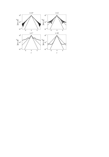
Figure 1: The distribution of the probability density in space for four different times: $t=0.07,0.2,0.7$ and $t=100$. The green dashed line represents the initial states $\left|{\psi\left({x,0}\right)}\right|^{2}$, the red dash-dotted line is the final bound state $\left|{\psi\left({x,\infty}\right)}\right|^{2}$, and the solid blue line is $\left|{\psi\left({x,t}\right)}\right|^{2}$.

On the other hand, when $\mu=0$, after the transition (the abrupt change) the potential vanishes and the wavefunction propagates freely in space

$$\psi\left({x,t}\right)=$$ (5)

$$\frac{1}{2}e^{it}\left\{{e^{-\left|x\right|}\mbox{erfc}\left[{\sqrt{it}-\frac{\left|x\right|}{2\sqrt{it}}}\right]+e^{\left|x\right|}\mbox{erfc}\left[{\sqrt{it}+\frac{\left|x\right|}{2\sqrt{it}}}\right]}\right\}$$

This is a relatively simple but important case (due to its generic nature), so we would like to elaborate on its dynamics.

In this case $\left|{\psi\left({x,0}\right)}\right|^{2}$ and $\left|{\psi\left({x,t}\right)}\right|^{2}$ are similar (except for the oscillations) only till a certain $x$, beyond which the wavefunction decays like $\left|{\psi\left({x,t}\right)}\right|^{2}\sim x^{-2}$ since for $x^{2}/t>>1$

$\psi\left({x,t}\right)\cong\frac{1}{\sqrt{i\pi t}}\frac{\exp\left({ix^{2}/4t}\right)}{1+\left({x/t}\right)^{2}}$.

This result is consistent with the prediction of ref.GranotMarchewka_12 that the wavefunction at very short times and long distances, i.e., $x^{2}/t>>1$, is

$\psi\left({x,t}\right)\sim\left[{\psi^{\prime}\left({0+,0}\right)-\psi^{\prime}\left({0-,0}\right)}\right]\frac{t^{3/2}}{\sqrt{i\pi}x^{2}}\exp\left({i\frac{x^{2}}{4t}}\right)$

(the initial exponentially small value of the wavefunction at $x\to\infty$ was ignored). When $0<\mu<1$ the dynamics is more intricate since the final states can be either extended (as in the $\mu=0$ case) or localized (Eq.2). The plot of the probability density $\left|{\psi\left({x,t}\right)}\right|^{2}$ as a function of $x$, as depicted in Fig.1 illustrates this point.

When the perturbation is turned on the initially localized particle’s energy is modified and the particle can remain localized at a different energy, i.e., $E_{0}^{f}=-\mu^{2}$ (instead of the initial one $E_{0}^{i}=-1)$ but it can also escape to the continuum.

At short times, $t<<x^{2}$ the wavefunction can be approximated by

$$\psi\left({x,t}\right)\cong e^{it-\left|x\right|}-4\left({1-\mu}\right)\\ \frac{\left({it}\right)^{3/2}}{\sqrt{\pi}}\frac{\exp\left({i\mu^{2}/4t}\right)}{x^{2}}$$ (6)

For $x\to\infty$ the wavefunction’s pertrubative term decays like $x^{-2}$. In Eq.6 we see that the short time behavior have a fractional power law and deviates from the reversible $t^{2}$ dependence CohenTannoudjietal_8 .

Figure 2: The temporal revolution of the probability density for $\mu=3$ (solid line). The dashed line stands for its final value $P\left({t=\infty}\right)$.

In the long time regime, i.e., $t\to\infty$, the wavefunction can be approximated

$$\psi\left({x,t}\right)\cong\left({\mu^{-1}-1}\right)\sqrt{\frac{i}{\pi}}\left|x\right|t^{-3/2}\exp\left({ix^{2}/4t}\right)+$$

$$\frac{4\mu}{1+\mu}\exp\left({i\mu^{2}t-\mu\left|x\right|}\right).$$

We observe two different dynamics regimes. At very large distances from the origin (but still $t>>x)$ the first term, which is related to the propagating-waves rules, while at short distances the first term is merely an oscillating correction to the second one, which is related to the final localized state. As $t\to\infty$ the wavefunction converges to the final bound state (3) with extra factor of $4\mu^{3/2}/\left({\mu+1}\right)$.

Usually, the measured quantity, which quantify the decay rate, is the survival amplitude $A\left(t\right)=\int\limits_{-\infty}^{\infty}{\psi^{\ast}\left({x,0}\right)\psi\left({x,t}\right)dx}$; and the survival probability $P\left(t\right)=\left|{A\left(t\right)}\right|^{2}$ is the probability to remain in the initial state (i.e., the non-decay probability); similarly, $1-P\left(t\right)$ is the probability to escape to infinity, i.e., to decay.

$A\left(t\right)$ can be calculated exactly and straightforwardly (albeit with tedious calculations). For the initial state ($\psi_{Bi}\left({x,t}\right)$) we find:

$$A\left(t\right)=\frac{1}{\left({1+\mu}\right)^{2}}$$ (7)

$$\left\{{\mbox{erfc}\left({\sqrt{it}}\right)\left[{1+\mu^{2}-2it\left({1-\mu^{2}}\right)}\right]+2\left({1-\mu^{2}}\right)\sqrt{\frac{it}{\pi}}e^{-it}+2\mu e^{it\left({\mu^{2}-1}\right)}\left[{2-\mbox{erfc}\left({\sqrt{it}\mu}\right)}\right]}\right\}$$

For completeness we add the special $\mu=0$ case:

$$A\left(t\right)={\mbox{erfc}\left({\sqrt{it}}\right)\left[{1-2it}\right]+2\sqrt{\frac{it}{\pi}}e^{-it}}$$ (8)

In Fig.2 the dynamics of the survival probability is presented for $\mu=3$. It is clear from the figure that the probability decays eventually irreversibly to a constant value. However, it never decays exponentially.

At long time the survival amplitude goes like

$$A\left({t\to\infty}\right)\sim\frac{4\mu e^{it\left({\mu^{2}-1}\right)}}{\left({1+\mu}\right)^{2}}\left[{1+\frac{\left({\mu-\mu^{-1}}\right)^{2}}{4\mu\pi^{1/2}\left(t\right)^{3/2}}e^{-it\mu^{2}-i3\pi/4}}\right]$$

and the non-decay probability can be approximated

$$P\left(t\right)=\left|{A\left({t\to\infty}\right)}\right|^{2}\sim$$

$$\frac{\left({4\mu}\right)^{2}}{\left({1+\mu}\right)^{4}}\left[{1+\frac{\left({\mu-\mu^{-1}}\right)^{2}}{2\mu\pi^{1/2}\left(t\right)^{3/2}}\cos\left({t\mu^{2}+3\pi/4}\right)}\right]$$

It oscillates with angular frequency $\mu^{2}$ with varying amplitude that decays like $t^{-3/2}$ and converges to the value $P\left(t\right)\to\frac{16\mu^{2}}{\left({\mu+1}\right)^{4}}.$

It should be noted that this final probability is smaller than 1 for either $\mu>1$ or $\mu<1$. This result obviously contradicts the classical intuition that the non-decay probability decreases only when the well is raised.

Despite the irreversible nature of the process, it has no similarity to the well-known exponential decay.

At short times $t<<1$ this expression can be expanded by fractional powers series to

$$A\left({t<<1}\right)\sim 1+2it\left({\mu-1}\right)+\frac{8\left({-1}\right)^{3/4}\left({\mu-1}\right)^{2}t^{3/2}}{3\sqrt{\pi}}-$$

$$\left({\mu-1}\right)^{2}\mu t^{2}-\frac{8\left({-1}\right)^{1/4}\left({\mu-1}\right)^{2}\left({2\mu^{2}-1}\right)t^{5/2}}{15\sqrt{\pi}}+\cdots.$$

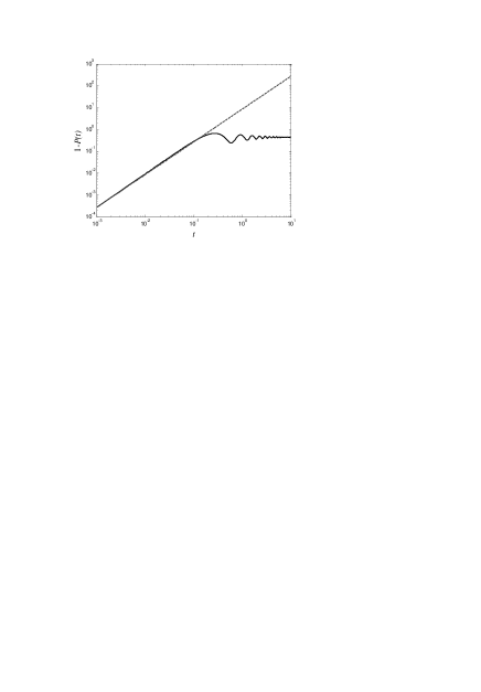
Figure 3: The escape probability $1-P\left(t\right)$ as a function of time (the solid black line) for $\mu=3$. The dashed red line stands for the short time approximation (Eq.9).

Therefore the non-decay probability goes like

$$1-P\left({t<<1}\right)=1-\left|{A\left({t<<1}\right)}\right|^{2}\sim\frac{8}{3}\sqrt{\frac{2}{\pi}}\left({\mu-1}\right)^{2}t^{3/2}$$ (9)

which means that the leading term in the escape probability has a fractional power dependence on time (see Fig.3).

This behavior resembles Chiuetal_3 where the dynamics of an ad-hoc potential spectrum was investigated; however, one of the advantages of the model present here is its physical realization. To the best of our knowledge, this model is the only decay model, which allow for an exact explicit analytical solution.

The $\mu\to 1$ regime calls for comparison with perturbation methods, which lead to the Fermi Golden Rule. In the latter case the short time regime goes like $t^{2}$ instead of $t^{3/2}$ of Eq.9.

As was said at the beginning of the paper, it should be stressed that even if the well had a finite width $\Delta x$ (instead of a delta function one), then the fractional behavior, which appears at Eqs.7-9 would still be traced for every shallow potential well (i.e., $|E_{0}|\sim(U_{0}\Delta x)^{2}/4<<\Delta x^{-2}$), and it is not merely a mathematical anomaly.

To summarize, the dynamics of a perturbed delta function potential well was investigated. Although this scenario can model a realistic case (such as a particle decay from a point potential trap), it has an exact analytical solution. Not only does this model behave differently than the well-known exponential decay law as classical decay laws predict, but it does not even have an integral power law at short times as quantum processes suggest. In fact, the dynamics is more intricate and has a fractional power law at short times.
We believe that the analyticity of the solution of this model along with its experimental feasibility can be used to shed light on the generic decay process from both practical as well as theoretical perspectives.

References

(1) L. Fonda, G.C. Ghirardi, and A. Rimini, Rep. Prog.
Phys.41, 587 (1978)
(2) P.T. Greenland, Nature335, 298 (1988)
(3) C.B. Chiu, E.C. G. Sudarshan, and B. Misra, Phys. Rev.
D16, 520-529 (1977)