Bright flares from the X-ray pulsar SWIFT J1626.6–5156

Abstract

Aims. We have performed a timing and spectral analysis of the X-ray pulsar SWIFT J1626.6–5156 during a major X-ray outburst in order to unveil its nature and investigate its flaring activity.

Methods. Epoch- and pulse-folding techniques were used to derive the spin period. Time-average and pulse-phase spectroscopy were employed to study the spectral variability in the flare and out-of-flare states and energy variations with pulse phase. Power spectra were obtained to investigate the periodic and aperiodic variability.

Results. Two large flares, with a duration of $\sim$450 seconds were observed on 24 and 25 December 2005. During the flares, the X-ray intensity increased by a factor of 3.5, while the peak-to-peak pulsed amplitude increased from 45% to 70%. A third, smaller flare of duration $\sim$180 s was observed on 27 December 2005. The flares seen in SWIFT J1626.6–5156 constitute the shortest events of this kind ever reported in a high-mass X-ray binary. In addition to the flaring activity, strong X-ray pulsations with $P_{\rm spin}=15.3714\pm 0.0003$ s characterise the X-ray emission in SWIFT J1626.6–5156. After the major outburst, the light curve exhibits strong long-term variations modulated with a 45-day period. We relate this modulation to the orbital period of the system or to a harmonic. Power density spectra show, in addition to the harmonic components of the pulsation, strong band-limited noise with an integrated 0.01-100 Hz fractional rms of around 40% that increased to 64% during the flares. A weak QPO (fractional rms 4.7%) with characteristic frequency of 1 Hz was detected in the non-flare emission. The timing (short X-ray pulsations, long orbital period) and spectral (power-law with cut off energy and neutral iron line) properties of SWIFT J1626.6–5156 are characteristic of Be/X-ray binaries.

Conclusions.

1 Introduction

SWIFT J1626.6–5156 was first detected on December 18, 2005 by the SWIFT satellite during an X-ray outburst (Palmer et al. 2005). The source showed X-ray pulsations with period $\sim$ 15 s and strong flaring activity. The spectrum was consistent with a power law with $\Gamma\approx 3.2$, giving $F_{X}=6.1\times 10^{-9}$ erg cm^-2 s^-1 in the energy range 15-100 keV. Subsequent observations (see Table 1) showed that SWIFT J1626.6–5156 is a highly variable source with a pulse period of 15.37682$\pm$0.00005 s (Markwardt & Swank 2005) and pulse fraction that increases from $\sim$50% between flares to $\sim$80% during the flares (Belloni et al. 2006). The X-ray spectrum is well fitted by an absorbed power-law component and a high-energy cutoff. An iron line at 6.4 keV is also detected (Markwardt & Swank 2005; Belloni et al. 2006). However, the values of the spectral parameters differ considerably between observations. Markwardt & Swank (2005) gave $E_{\rm cutoff}=5$ keV and $N_{\rm H}=2\times 10^{22}$ cm^-2, whereas Belloni et al. (2006) gave $E_{\rm cutoff}=12$ keV and $N_{\rm H}=5\times 10^{22}$ cm^-2. Campana et al. (2006) did not detect the iron line nor a cutoff. These authors reported a harder and less absorbed spectrum ($\Gamma=0.7$, $N_{\rm H}=0.95\times 10^{22}$ cm^-2). Finally, an INTEGRAL spectrum in the range 4-60 kev obtained by Tarana et al. (2006) gave $\Gamma=0.6$, $E_{\rm cutoff}=6.7$ keV. The optical counterpart is believed to be 2MASS16263652–5156305 (Rea et al. 2006; Negueruela & Marco 2006), a Be star showing strong H_α emission. A Chandra observation confirmed that the position of the X-ray source is consistent with the suggested counterpart. Chandra coordinates are RA: 16h26m36.5s, Dec: -51d56m30.7s, with an error of 0.6 arcsec (Homan, private communication).

In this work we present the results of a timing and spectral analysis of SWIFT J1626.6–5156 using RXTE data, limited to the three observations early in the outburst where flares are observed. The details of the observation are explained in Sect. 2 and a log presented in Table 2. In Sect. 3 the periodic and aperiodic time variability of SWIFT J1626.6–5156 is investigated. Sect. 4 deals with the time-average and pulse-phase spectral variability. In Sect. 5 a comparison of the timing and spectral properties of the flare and out-of-flare emission is performed and the nature of the system is discussed.

Table 1: X-ray observations of SWIFT J1626.6–5156 in the literature and best-fit spectral parameters of an absorbed power law with cutoff.

Date	Satellite	Fluxa	Energy range	$\Gamma$	$E_{\rm cut}$	$N^{b}_{\rm H}$	Fe line	Reference
			(keV)		(keV)		(keV)
18-12-2005	SWIFT	6.1	15-100	3.2	-	-	-	Palmer et al. (2005)
19-12-2005	RXTE	4.1	2-40	0.9	5	2	6.4	Markwardt & Swank (2005)
19-12-2005	RXTE	3.6-2.4	3-25	0.9-1.3	12	4-5.5	6.4	Belloni et al. (2006)
12-01-2006	SWIFT	1.2	0.5-10	0.67	-	0.94	-	Campana et al. (2006)
21-01-2006	INTEGRAL	1.6	4-40	0.6	6.7	-	-	Tarana et al. (2006)
$a$: $\times 10^{-9}$ erg cm-2 s-1
$b$: $\times 10^{22}$ cm-2

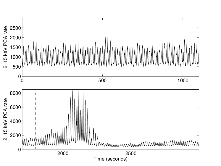
Figure 1: Light curve of Obs. 1 showing the X-ray pulsations and the increase of the pulse fraction during the flare event. Bin size is 1 s. The dashed lines mark the flare interval used in the analysis (see text).

Figure 2: Light curves and hardness-intensity diagrams of the three observations. The Y-axis was left the same in the three panels to allow easy comparison. The entire time interval is used with a bin size of 64 s. The dashed lines indicate the limits of the pre-, post- and flare intervals selected for the analysis.

2 Observations and data analysis

SWIFT J1626.6–5156 was observed with the Proportional Counter Array (PCA) onboard the Rossi X-ray Timing Explorer (RXTE) starting from December 19, 2005, one day after the discovery by Swift. Here we concentrate on the three observations made between December 24-27, 2005 (MJD 53728.385–53731.295), in which the source displayed flaring activity. The data correspond to RXTE proposal P91094. Four PCUs were on during the entire duration of the three observation intervals. PCU1 was off all the time.

Light curves and spectra were extracted using version v.5.3.1 of the RXTE FTOOLS package. The following screening criteria were applied to the data prior extraction: good time intervals were defined when the pointing of the satellite was stable ($<0.02^{\prime\prime}$), the elevation above 10^∘ and far away from the South Atlantic Anomaly.

The log of the observations is given in Table 2. Each observation contains one flare event, although the event that took place in Obs. 3 was significantly smaller and shorter. The duration of the flares varied from $\sim$180 to 480 s. The flare in Obs. 2 was detected at the end of the observation interval. Thus, the duration of post-flare interval of Obs. 2 is short ($\sim$ 100 s). The pre-flare interval of Obs. 3 contains a data gap of about 2260 s due to the passage through the SAA anomaly.

Table 2: Summary of the observations.

Obs.	RXTE ID	MJD	MJD	Pre-flare			Flare			Post-flare
interval		start	end	$I_{X}^{a}$	Duration	PF	$I_{\rm peak}$a	Duration	PF	$I_{X}^{a}$	Duration	PF
1	91094-02-02-01	53728.385	53728.425	995	1800	44%	3555	450	72%	750	1142	31%
2	91094-02-02-02	53729.168	53729.211	988	2900	46%	3880	480	70%	600	108	36%
3	91094-02-02-04	53731.228	53731.295	680	2057	38%	1040	180	51%	645	1236	37%
$a$: Background-subtracted count rate for 4 PCU in the energy range 2-15 keV for a time bin of 16 s.
Durations are in seconds.

3 Timing analysis

3.1 Light curves and hardness ratios

Strong pulsations are detected at the 15.37s period from all observations. Figure 1 shows the light curve of Obs. 1 at high resolution ($\Delta t=1$ s). The top panel shows the first 1.2 ks of data, where the pulsation is evident. The bottom panel shows the second part of the observation, which includes a strong flare. Its shape is very similar to that of the other strong flare (from Obs. 2): a major increase in the pulsed fraction, clearly accompanied by a more moderate increase of the DC level, followed by a depression of DC level and pulsed fraction and a slow recovery. Fig. 2 shows the three flare events with corresponding hardness-intensity diagrams using a coarser time bin ($\Delta t=64$ s). The hardness ratio was defined as the ratio between the count rate in the 9-15 keV band to the count rate in the 2-9 keV band. The flare in Obs. 2 is very similar to that in Obs. 1, although it appears later in the observation and the post-flare region is not observed. The flare in Obs. 3 is much weaker. As the count rate increases, the hardness ratio increases until the count rate reaches about 350 c s^-1 at which point it flattens. The dashed lines in Fig. 1 and 2 indicate our definition of pre-flare, flare and post-flare intervals for each observation.

As mentioned, during the flares, the pulsed fraction increases considerably; the minima of the pulsation cycle increase by a factor of 2, while the maxima increase by a factor of 5. After the flares, both the average rate and the pulsed fraction go below their pre-flare values, and start a slow recovery. In Obs. 1 the flux had not completely recovered the pre-flare level 1200 seconds later, when the observation ended. Given the fact that the pre-flare level of Obs. 2 is similar to that of Obs. 1, it is likely that the source intensity fully recovered to the pre-flare level.

In order to investigate differences in the emission properties between the flare and quiescent states, we isolated the time intervals corresponding to the flare events. For each observation, we defined three intervals: pre-flare, flare and post-flare. The exact definition of these intervals can be seen in Fig. 2.

The average count rate (peak intensity in the case of the flare interval), duration and pulse fraction of the available intervals corresponding to the three ”states” (pre-flare, flare and post-flare) for each observation are given in Table 2.

3.2 Spin period determination

In order to determine the spin period of SWIFT J1626.6–5156 we obtained a 0.125-s binned barycentric corrected light curve of the non-flaring emission for the three observation intervals in the energy range 2-15 keV (from PCA B_2ms_8B_0_35_Q mode). An FFT applied to the light curve revealed a coherent modulation at 0.065 Hz, which correspond to a pulse period of 15.4 s. Several of its harmonics are clearly seen. In order to accurately measure the pulse period, a pulse-folding analysis was performed. The light curve was divided into blocks of continuous stretches of data points with a duration of 230 s. Each block was folded modulo the initial period found from the FFT. The resulting pulse profile obtained for the first block was used as a template. The difference between the actual pulse period at the epoch of observation and the period used to fold the data was determined by cross-correlating the pulse profiles corresponding to each block and the template. The phase shifts were fitted to a linear function, whose slope represents the correction in frequency to the actual period. A new template was derived for this corrected period, and the process repeated. The derived pulse periods were 15.3718$\pm$0.0003 s, 15.3711$\pm$ 0.0002 s and 15.3724$\pm$0.0007 s for the three observations, respectively.

3.3 Pulse profile and pulse fraction

The average pulse profiles at three different energy ranges, obtained by folding the corresponding light curves onto the best-fit spin period, are shown in Fig. 3. The pulse profile of the flare is somehow narrower than that of the out-of-flare but for both there is no strong dependence on energy. The pulse fraction was calculated as PF =($I_{max}$–$I_{min}$)/($I_{max}$+$I_{min}$).

Figure 3: Comparison of the pulse profile as a function of energy during the flare (right) and non-flaring (left) part of the light curve. Data correspond to Obs 1.

In order to perform a more in-depth analysis of the individual pulse profiles, we extracted a light curve from the full PCA energy range with a bin size of $P_{\rm spin}/20$, divided it in intervals 20-points long (centered approximately on the pulse maximum) and with these constructed a time-phase image, with time on the X-axis, pulse phase on the Y-axis and count rate on the Z axis. The image on a gray scale color map is shown in Fig. 4, together with the corresponding light curve (top panel). From this figure, one can see that the out-of-flare pulse peaks at around phase 0.5, while the flare itself is characterized by a maximum around phase 0.6. Moreover, at T$\sim$500 one can see a small rate increase corresponding to a slightly higher phase, indicating that a very small flare is probably present there.

In order to study in more detail the pulse changes during the flare, we accumulated an out-of-flare template by simply adding the first 100 cycles. Comparing this template with the single pulses during the flare, it appears as if the flare could be characterized by the appearance of one or two additional components at fixed phases.

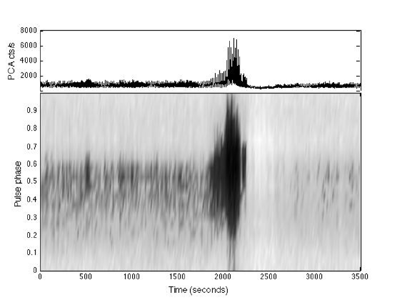
Figure 4: Top panel: light curve of Obs. 1. Bottom panel: corresponding time-phase image, obtained aligning all pulses as a function of time. Darker areas indicate higher count rate.

In order to assess this numerically, we ran the following procedure. Each cycle was fitted with the out-of-flare template with a variable overall multiplicative factor. Not surprisingly, outside the flare and post-flare region (and with the exception of three cycles around cycle 35), this model gives a decent fit with normalization equal to 1. By decent fit we mean a fit with a $\chi_{r}^{2}=\chi^{2}$/20 $<$15: this is not formally acceptable, but no systematic residuals are seen and given the high statistics it can not be expected that a single simple model could fit all single cycles. Overall, out of flare the $\chi^{2}_{r}$ values are around 8.

For the cycles with $\chi^{2}_{r}>15$, we identify the largest positive deviation from the template fitting (limited to the phase range 0.2-0.8) and repeat the fit with the addition of a Gaussian component centered at the position of that maximum deviation, with normalization equal to the maximum deviation and with starting width 0.1. With this addition, only a few cycles around the maximum of the flare retain a $\chi^{2}_{r}>15$.

In order to try to find a better fit for these cycles, we added an additional Gaussian component. The procedure is the same as before. The new Gaussian is added only if the fit with a single Gaussian results in a $\chi^{2}_{r}>15$. The fits are considerably better during the flare, although there are still a few points with a $\chi^{2}_{r}>15$. The $\chi^{2}_{r}$ values obtained with this procedure are shown in Fig. 5.

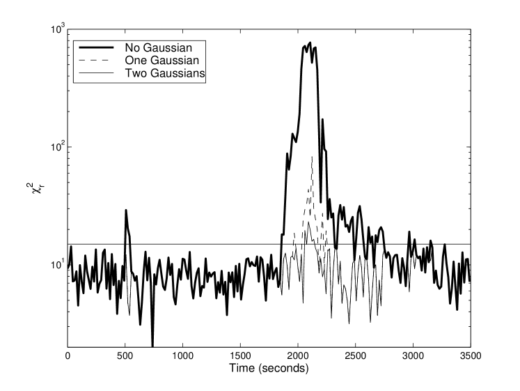
Figure 5: Values of $\chi^{2}_{r}=\chi^{2}/20$ obtained with the fitting procedure described in the text. The different curves correspond to simple template (dotted line), template plus one Gaussian (dashed line) and template plus two Gaussians (full line). The horizontal line marks the level $\chi^{2}_{r}=15$.

The final fits have a number of free parameters between one (the template normalization factor for the template-only fits) and seven (template normalization plus three parameters for each of the two Gaussians) for the most complex fits. The best fit values for five of the seven parameters are shown in Fig. 6. The remaining two parameters, the width of the two Gaussians, are clustered around 0.1-0.2 and 0.01-0.05 in phase for the first and second Gaussian respectively.

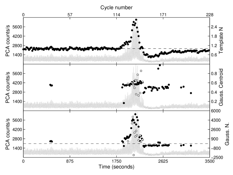
Figure 6: Best fit parameters as a function of time. On all three panels, the gray curve shows the PCA count rate evolution for reference. Top panel: multiplicative factor for the out-of-flare template. The dashed line shows the level of 1. Middle panel: phase of the centroid of the Gaussians (first Gaussian: filled circles; second Gaussian: empty circles). Bottom panel: normalization of the Gaussians (first Gaussian: filled circles; second Gaussian: empty circles). The dashed line corresponds to zero normalization.

Based on these results, we can identify three intervals:

• Before the flare: the pulse shape is consistent with a constant shape, corresponding to what we used as template.

• During the flare: the template shows a higher normalization factor (up to 3), while an additional broad Gaussian centered at phase 0.6 appears. Occasionally, a second narrower Gaussian is necessary for a fit.

• During the post-flare depression: the template normalization is lower than unity and a negative Gaussian with a very constant normalization is apparent.

• After the post-flare depression: the template normalization slowly recovers to unity, no Gaussians are needed.

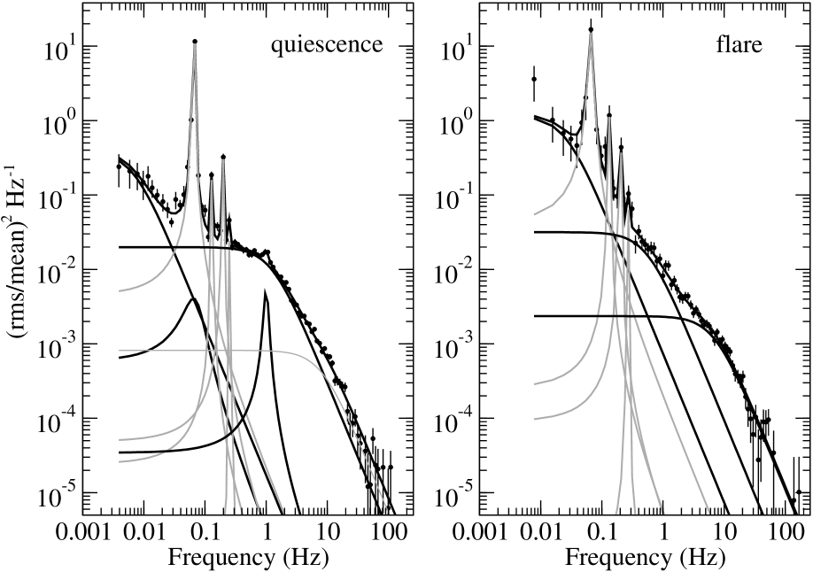
Figure 7: Power spectrum of SWIFT J1626.6–5156. Coherent pulsations are clearly seen at $\sim$0.065 Hz together with some higher harmonics. The quiescence emission shows a weak QPO components at 1 Hz. The lines indicate the Lorentzian components used to fit the power spectra (see text)

3.4 Power spectrum and noise components

In order to obtain the power spectra, the Obs. 2 light curve was binned with bin size $2^{-9}$ s, which is the maximum resolution provided by the B_2ms_8B_0_35_Q data mode. Then the light curve was divided into segments of 512 s for the non-flare part and 128 s for the flare. An FFT was calculated for each segment (6 for the non-flare and 4 for the flare). The final power spectra resulted after averaging all the individual power spectra and rebinning in frequency. Figure 7 shows the power spectra and noise components of the preflare and flare light curves. In addition to the harmonic components of the pulsations, strong band-limited noise is detected both in the quiescence (i.e. non-flaring emission) and during the flare, with an integrated 0.01-100 Hz fractional rms of around 40% and 64%, respectively. The change in the pulse profile between pre-flare and flare (as seen in Fig. 3) can also be expected from the change in the relative strength of the harmonics of the pulsation.

The power spectra were fitted with Lorentzians. Ignoring the X-ray pulsation and its harmonics, a total of 5 Lorentzians were required to fit the non-flare power spectrum, while the flare power spectrum needed 3 Lorentzians.

Three Lorentzians are common to the two data sets. These are zero-centred Lorentziants that fit the continuum. The power spectra of the non-flare part require two more Lorentzians. One is centred at the same frequency as the pulsation and can be interpreted as the coupling between the periodic and aperiodic variability (Lazzati & Stella 1997). This coupling can be recognised by the broadening of the wings of the narrow peaks of the periodic modulation. The lack of this component in the flare power spectrum maybe due to the fact that the aperiodic noise is stronger (see the higher continuum short-ward of the pulsation) during the flare. The non-flare power spectrum presents a QPO at around $\nu=1$ Hz with Q ($\nu$/FWHM) of 4 and fractional rms amplitude of 4.7%.

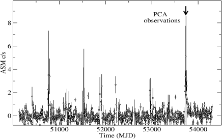
Figure 8: 5-d binned ASM light curve of SWIFT J1626.6–5156 for the period MJD 50135–54340. The start time of the PCA observations is indicated by an arrow.

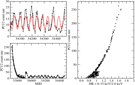
Figure 9: After the outburst that led to its discovery as an X-ray source, SWIFT J1626.6–5156 exhibited a periodic modulation with period $\sim$45 days. On the right the hardness ratio-intensity diagram is shown.

3.5 Longer-term variability

Figure 8 shows the long-term variability of SWIFT J1626.6–5156 and the transient nature of its X-ray emission. The source spends most of the time in a quiescent state (the average count rate is $\approx$0.06 ASM c s^-1) and only occasionally goes into outburst. Note that significances above 3 sigma are only seen in the 5-day average ASM bins that cover the 2005 December outburst.

We also collected the average PCU2 count rates for each of the 295 RXTE observations, thus resulting in an unevenly spaced time series (see Fig. 9). The onset of the PCA observations coincided with the outburst peak (Fig. 8). A first visual inspection of the resulting lightcurve shows two main properties: i) an initial fast flux decay lasting for about 160 days since the outburst onset, followed by ii) a series of apparently periodic ”bumps”. In order to carry out a first estimate of the two components we fitted the first 160 day points with an exponential component and the second part of the lightcurve with a sinusoid. For the first component we found that $\tau$ of the exponential is $\sim$33 days. For the second component we obtained a period of 45$\pm$1 days, though the reduced $\chi^{2}$ is only about 2.

We note that bumps are rather asymmetric, suggesting either that the sinusoid model is a rough estimate of the raw data and/or the 45-d period is a harmonic of the true period. This interpretation is also corroborated by the very high asymmetric profile of the latest four peaks, with the odd and even bumps differing each other. To test this hypothesis we add an additional sinusoidal component to the fit with a period forced to be twice to that of the first component. The inclusion of this component has a probability of $\sim$99.0% to be significant. It is evident that only future optical spectroscopic studies of the companion star and/or pulse arrival time analysis of the X-ray photons can provide an unambiguous detrmination of the orbital period. The first bump after the exponential flux decay phase is a reminiscence of what is routinely observed in many Be/X-ray binaries as they enter in an outburst phase (see e.g. Campana et al. 1999): a rapid rise in flux, a flat topped maximum and a relatively slow decay. At variance with the above interpretation is the second bump which falls at the minimum of the expected modulation.

Figure 9 also shows the variation of the hardness of the source, defined as the ratio between the count rates in the energy bands 6-15 keV to 2-6 keV, as a function of intensity. As the outburst decayed the source became softer .

It is worth mentioning that the same flare mechanism that occurs during high-intensity states, i.e., near the outburst peak, still works at lower mass accretion rates. The variability seen at the end of the outburst decay, around MJD 53800-53900 (see Fig. 9), is caused by the same type of flaring activity that we have reported in previous sections. The flares show the same factor 3-4 increase in flux and also an increase in the pulse fraction.

Table 3: Results of the fits to the power spectra. Only the non-coherent components are shown.

Lorentzian	quiescence	flare
$\nu_{1}$ (Hz)	0f	0f
$FWHM_{1}$ (Hz)	0.013$\pm$0.007	0.012$\pm$0.009
rms1 (%)	7.8$\pm$1.3	38.7$\pm$9.0
$\nu_{2}$	0.065f	–
$FWHM_{2}$	0.4${}^{+3.4}_{-0.2}$	–
rms2	5.4$\pm$1.9	–
$\nu_{3}$	1.02$\pm$0.03	–
$FWHM_{3}$	0.23$\pm$0.07	–
rms3	4.7$\pm$1.0	–
$\nu_{4}$	0f	0f
$FWHM_{4}$	2.4$\pm$0.2	1.0$\pm$0.3
rms4	26.2$\pm$1.0	24.9$\pm$1.6
$\nu_{5}$	0f	0f
$FWHM_{5}$	13.7$\pm$1.3	13.5$\pm$1.7
rms5	15.9$\pm$1.0	22.3$\pm$0.9
$f$: fixed

4 Spectral analysis

4.1 Time-averaged spectroscopy

In order to investigate potential spectral variability between the non-flare emission and the emission during the flare, we extracted energy spectra corresponding to the flare and a stretch of non-flare emission. Fig. 10 shows the spectra for Obs.1 and Table 4 summarises the results of the spectral fits for the three observations. A systematic error of 1% was added in quadrature to the statistical one. An absorbed power law with a high-energy cut off and an iron line at $\sim 6.4$ keV provided a good fit to the spectral continua. No spectral variability is seen within the uncertainties, although the flare spectrum in Obs. 2 is somehow harder than the preflare one. The pre-flare and flare spectra basically differ in that the pre-flare spectra require the inclusion of an edge at $\sim$9 keV to obtain an acceptable fit. The probability that the improvement of the fit occurs by chance (F-test) by the addition of this component is $\mathbin{\lower 3.0pt\hbox{$\hbox to0.0pt{\raise 5.0pt\hbox{$\char 60\relax$}\hss}\mathchar 29208\relax$}}10^{-5}$.

Table 4: Spectral fits results for the three observations. Uncertainties are 90% confidence. Flux corresponds to the energy range 3-30 keV.

	Obs. 1		Obs. 2		Obs. 3
parameters	pre-flare	flare	pre-flare	flare	pre-flare	flare
Flux (erg cm-2 s-1)	$3.5\times 10^{-9}$	$8.4\times 10^{-9}$	$3.5\times 10^{-9}$	$6.3\times 10^{-9}$	$3.1\times 10^{-9}$	$3.8\times 10^{-9}$
$N_{H}$ ($\times 10^{21}$ cm-2)	9.4∗	9.4∗	9.4∗	9.4∗	9.4∗	9.4∗
$\Gamma$	0.73${}^{+0.08}_{-0.05}$	0.6$\pm$0.1	0.8$\pm$0.1	0.5$\pm$0.1	0.82$\pm$0.06	0.8$\pm$0.1
norm.	0.11$\pm$0.01	0.22$\pm$0.03	0.12$\pm$0.01	0.15$\pm$0.02	0.12$\pm$0.01	0.13$\pm$0.02
$E_{cut}$ (keV)	4.7$\pm$0.3	4.8$\pm$0.4	5.0${}^{+0.1}_{-0.4}$	4.5$\pm$0.4	5.0$\pm$0.3	5.0$\pm$0.4
Efold (keV)	9.7${}^{+0.8}_{-0.4}$	8.6$\pm$0.6	10.3$\pm$0.5	8.2${}^{+0.6}_{-0.3}$	10.0${}^{+0.8}_{-0.5}$	10.6${}^{+1.4}_{-0.8}$
$E_{\rm Fe}$ (keV)	6.2$\pm$0.1	6.5$\pm$0.2	6.3$\pm$0.1	6.4$\pm$0.1	6.3$\pm$0.1	6.4$\pm$0.1
$\sigma_{\rm Fe}$ (keV)	0.4∗	0.4∗	0.4∗	0.4∗	0.4∗	0.4∗
norm. ($\times 10^{-3}$)	6$\pm$1	8$\pm$3	5.2${}^{+1}_{-0.6}$	9$\pm$2	5$\pm$1	7$\pm$1
EW(Fe) (eV)	195$\pm$30	105$\pm$30	180$\pm$30	160$\pm$20	195$\pm$35	235$\pm$80
$E_{\rm edge}$ (keV)	8.7${}^{+0.8}_{-0.4}$	–	8.9$\pm$0.5	–	8.9$\pm$0.5	–
$\tau_{\rm edge}$	0.07$\pm$0.03	–	0.07$\pm$0.02	-	0.06$\pm$0.02	–
$\chi^{2}_{r}$(dof)	0.98(46)	0.85(48)	0.99(46)	0.91(48)	0.82(48)	1.15(48)
*: fixed

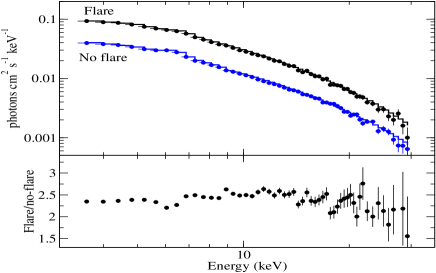
Figure 10: Energy spectra of the flare and out-of-the-flare parts for Obs 1. The lower panel shows the ratio between the two spectra.

4.2 Pulse-phase spectroscopy

As mentioned above, the shape of the pulse profile of SWIFT J1626.6–5156 hardly changes with energy. A more detailed way to investigate how the X-ray spectrum changes as a function of the spin of the magnetized neutron star is by performing pulse-phase spectroscopy. In order to investigate the pulse phase dependence, high time and energy resolution are needed simultaneously. Unfortunately, the only data mode available in our observations that provides detailed time and energy information is B_2ms_8B_0_35_Q, which provide high time resolution but modest energy resolution, namely, eight energy channels in the energy range 2.6-15 keV.

The pulse profile of Obs. 2 was divided into eight equally spaced bins to provide eight 2.6-15 keV background-subtracted spectra. Each spectrum was fitted with a power law plus iron line and edge. Due to the modest energy resolution, the iron line parameters were not well constrained. The iron line and edge energy were fixed to 6.4 keV and 8.8 keV, respectively, the value obtained from the time-average spectrum. As can be seen in Fig. 11, despite that the flux changed by a factor 2, no significant changes were seen in any of the spectral parameters, neither in the continuum (power-law photon index) nor in the line and edge (width, $\tau_{\rm edge}$). This result confirms the absence of variability of the pulse profiles with energy.

Figure 11: Spectral parameters as a function of pulse phase for the preflare state of Obs. 2.

5 Discussion

We have performed a timing and spectral analysis of the newly discovered X-ray pulsar SWIFT J1626.6–5156. We have concentrated on the observations made at the early phase of the reported outburst (see Fig. 8 and 9) in which the source displays flaring activity. Each X-ray light curve was divided into subintervals corresponding to the out-of-flare and flare parts of the observations. A separate analysis was carried out in each subinterval.

5.1 Out-of-flare analysis

The out-of-flare parts of the light curves were used to derive the spin period because these parts do not present high amplitude flux changes and because of their longer duration, allowing enough number of cycles to be included. No significant variations in the spin period were seen during the observations. Thus we derived a weighted mean spin period of 15.3714$\pm$0.0003 s.

The pulse profile of the out-of-flare part of the X-ray light curve, obtained by considering 100 cycles folded on the spin period, and a variable overall multiplicative factor fits well the individual pulses with normalization equal to unity. In the case of the post-flare interval, where both the overall flux level and the pulse amplitude are depressed, the best fits are obtained with the addition of a negative Gaussian component.

The average non-flare X-ray flux in the 3-30 keV band is $3.5\times 10^{-9}$ erg s^-1 cm^-2 for Obs. 1 and Obs. 2 and slightly lower in Obs. 3, $2.9\times 10^{-9}$ erg s^-1 cm^-2. There is no clear evidence for variability of the spectral parameters with time nor between the flare and out-of-flare spectra in any of the three observations. The only difference is the presence of an absorption edge component in the out-of-flare spectrum that it is not required in the flare spectrum.

5.2 Flare analysis

The flare event consists of a sudden increase of the X-ray flux by a factor of four and is accompanied by an increase of the pulse fraction and a hardening of the spectrum. The average 3-30 keV flux, taking into account the entire duration of each flare, decreased from $8.5\times 10^{-9}$ erg s^-1 cm^-2 in Obs. 1 to $6.3\times 10^{-9}$ erg s^-1 cm^-2 in Obs. 2 and further to $3.8\times 10^{-9}$ erg s^-1 cm^-2 for Obs. 3.

The template fitting showed that the flare corresponds to the appearance of an additional component at a different phase than the “normal” pulse shape outside flares, in addition to a brightening of the out-of-flare template. The average pulse profile obtained before the flare does not generally fits well the individual pulses during the flare. The addition of a Gaussian component centered around phase 0.6 (shifted from the peak at phase 0.5 of the template shape) reduces largely (see Fig. 5) the amount of bad fits. Still, there are some pulses that do not fit well to an average profile plus a Gaussian. The addition of a second Gaussian improved further the fits during the flare. In the post-flare phase, when the template normalization goes below unity, this additional component disappears and is replaced by a negative Gaussian component centered at phase 0.5. As the template slowly recovers to pre-flare levels, the negative component also disappears.

This behavior is difficult to understand. The flare appears to be made of a general increase in the pulse fraction plus the appearance of a peaked component at phase 0.6. The relatively small difference in average energy spectrum between non-flare and flare indicates that the spectrum of the additional component is not very different from that of the template emission. The post-flare negative contribution shows that after the flare the additional Gaussian disappears and is replaced by a depression of the template maximum, together with a decrease of the pulse fraction.

5.3 The nature of the source

The X-ray spectral components of SWIFT J1626.6–5156, namely, absorbed power-law component plus high-energy cutoff and iron line at 6.4 keV are characteristics of accreting X-ray pulsars (White et al. 1983; Reig & Roche 1999; Coburn et al. 2002). Although a few low-mass X-ray pulsars are known (e.g. Her X–1) the vast majority of pulsating neutron star are found in high-mass X-ray binaries. Massive X-ray binaries are classified according to the luminosity class of the optical component into supergiant X-ray binaries and Be/X-ray binaries. The former tend to be persistent sources, have short ($P_{\rm orb}<10$ d) orbital periods and long spin periods ($P_{\rm spin}>100$ s), while Be/X-ray binaries are usually transients, have wider orbits ($P_{\rm orb}>20$ d) and contain fast rotating neutron stars ($P_{\rm spin}<100$ s). On long timescales Be/X-ray binaries display two types of X-ray activity: regular, orbitally modulated outbursts normally peaking at or close to periastron with X-ray flux increases of about one order of magnitude with respect to the pre-outburst state, reaching peak luminosities $L_{x}\leq 10^{37}$ erg s^-1 (type I) and bright (X-ray flux $10^{3}-10^{4}$ times that at quiescence) uncorrelated with orbital phase and that last for several orbital periods (type II).

The long-term variability of SWIFT J1626.6–5156 shown in Fig. 8 and 9 is reminiscent of Be/X-ray binaries (Reig 2007), especially, the detection of smaller periodic outbursts (type I) following a major one (type II). This behaviour has been seen in the Be/X-ray binaries 4U 0115+63 (Negueruela et al. 1998), KS 1947+300 (Galloway et al. 2004) and EXO 2030+375 (Reig 2008). The periodicity is associated with the orbital period of the system. The X-ray emission increases as a result of accretion from the circumstellar disk of the Be star during periastron passage. Therefore, it seems natural to assume that the small outbursts in SWIFT J1626.6–5156 are also separated by the orbital period. Nevertheless, given the asymmetric profiles of the outbursts (note the last four shown in Fig. 9), we cannot exclude that the true orbital period is twice the modulation. In fact, the optical counterpart to SWIFT J1626.6–5156 exhibits strong H$\alpha$ emission. Negueruela & Marco (2006) reported an H$\alpha$ equivalent width of $\sim$ –40 Å. Such equivalent width implies an orbital period $100<P_{\rm orb}<200$ days (Reig 2007). Although the H$\alpha$ line may also appear in emission in supergiant binaries, the equivalent width is normally below $\sim$7 Å in these systems.

We can then conclude that all the observational data available of SWIFT J1626.6–5156 both from the vicinity of the compact object (relatively short spin period, X-ray spectral parameters, transient X-ray emission) and the optical companion (strong H$\alpha$ emission, relatively long orbital period) suggest the presence of a neutron star orbiting a Be star companion.

If the nature of SWIFT J1626.6–5156 as a Be/X-ray binary is finally confirmed, then this is the first time that such superfast flaring activity is reported for this type of systems. Up to now the fastest X-ray variability seen in Be/X-ray binaries was that associated with the rotation of the neutron star (X-ray pulsations). Flaring activity is not uncommon in massive X-ray binaries habouring supergiant companions (SGXR) but absent, with only one exception (EXO 2030+375), in Be/X-ray binaries. During an X-ray outburst of the Be/X-ray binary EXO 2030+375 detected by EXOSAT in 1985 October, a series of six flares that recurred quasi-periodically every 3.96 hr were observed. The duration of these flares varied between 1.3-2.3 hr and showed significant variability during the decay, consisting of intensity quasi-priodic oscillations with periods of 900-1220 s (Parmar et al. 1989).

The flares of EXO 2030+375 share similar properties with those seen in LMC X-4 flares, including the $\sim$3-4 hr flare recurrence time, the $\sim$1-2 hr flare duration, the high fluences of the flares ($>10^{40}$ ergs), the rapid rise with gradual decay, and the absence of any significant spectral change (Moon et al. 2003). These similarities suggest a common origin. One possible mechanism could be Rayleigh-Taylor instabilities near the magnetospheric boundary of the neutron star (Apparao 1991).

Flaring activity has also been reported in two wind-fed supergiant X-ray binary. 4U 1907+09 exhibits flares on time scales of 1–2 hr (Fritz et al. 2006). These flares are locked to the orbital motion as they occur twice per orbit (in’t Zand et al. 1998; Mukerjee et al. 2001). Vela X–1 has been observed to flare above its persistent level on several occasions (Laurent et al. 1995; Krivonos et al. 2003). The duration of the flares was 5-6 hr.

However, the duration of the flares in the systems mentioned above is longer, typically by one order of magnitude, than the flares observed in SWIFT J1626.6–5156. It is their short duration and the fact that they occur in a system with a main-sequence companion what makes the event in SWIFT J1626.6–5156 unique.

Fast and short-lived flares have been also reported for the newly suggested class of supergiant X-ray binaries, known as supergiant fast X-ray transients, SFXT (Negueruela et al. 2006; Smith et al. 2006). As in the classical supergiant binaries these sporadic outbursts typically last for few hours (Sguera et al. 2006). They differ in that SFXTs are transient sources and in the complex structure of the outbursts, consisting of one or a few short flares. However, at least two SFXTs have shown flares with a duration comparable to that of SWIFT J1626.6–5156, namely XTE J1739–302 (Sakano et al. 2002) and IGR J17544–2619 (González-Riestra et al. 2004).

The physical explanation of the fast outbursts is not clear. Accretion from a smooth homogeneous stellar wind is ruled out. Instead, porous (clumpy) winds are invoked. Fast outbursts would be due to the accretion of large, dense clumps on the neutron star (Walter & Zurita-Heras 2007; Negueruela et al. 2008). Recently, Sidoli et al. (2007) has proposed the presence of a second wind component in the form of an equatorial disk around the supergiant donor to explain the outbursts seen in the SFXT IGR J11215–5952, the only SFXT that exhibits periodic outbursts. These outbursts last for about 10 days and exhibit flaring activity near the peak. They are reminiscent of the type I outbursts so common among Be/X-ray binaries and most likely have a complete different origin to that of the fast, short ($\sim 1$ hr) flares. Even Sidoli et al. (2007) suggest that the $\sim$1-hr duration flares seen at the peak of the longer outburst in IGR J11215–5952 can be ascribed to the clumpy nature of the wind in the equatorial disk.

The asymmetry of mass outflows in Be stars is well established (Waters et al. 1988). The structure of the stellar winds in Be stars contains two components: at higher latitudes, mass is lost through the high-velocity, low-density wind (typical of early-type stars); in the equatorial regions a slower and denser wind operates and ultimately forms the disk. The interaction between the neutron star and the equatorial disk gives rise to enhanced accretion and increase of the X-ray flux.

The short-lived flares in SWIFT J1626.6–5156 can then be explained by the interaction between the accreting compact object and a clumpy stellar wind. Whether this stellar wind is the polar or equatorial component is not clear and will probably depend on the geometry of the orbit. If the equatorial plane and orbital plane are not coplanar and the orbit is relatively wide (so that the compact object does not directly crosses the disk) then the neutron star will be exposed to the polar wind. The determination of the orbital parameters of SWIFT J1626.6–5156 may provide the key to understand the physical mechanism behind the flares.

Given the short duration of the flares in SWIFT J1626.6–5156 it is tempting to compare the SWIFT J1626.6–5156 properties with those of neutron star low-mass binaries, in particular those of the ”bursting pulsar” and the ”Rapid Burster” since these systems also show fast and short episodes of increase X-ray emission. Instead of the term ”flares” the word ”burst” is used in this context. Both systems are transient, and the accretor in both is a neutron star. Both show postburst ”dips” followed by a relatively long recovery interval preceding a further burst. This behavior can be understood in terms of depletion of the reservoir followed by a fill-in time. Though the burst duration is very long in the case of SWIFT J1626.6–5156 it is also interesting to note that burst durations up to 700 s have been detected from the Rapid Burster from type-II bursts. The longer bursts of Rapid Burster (comparable to those observed in SWIFT J1626.6–5156) have a recovery time of $\sim$1hr, clearly not covered by the relatively short (1hr) RXTE pointings.

Type II bursts likely originate by spasmodic release of gravitational potential energy, which is almost certainly due to some not yet understood accretion disk instability. In support of this similarity of bursts is the fact that the spectra of the burst and the persistent emission are nearly identical, suggesting a similar (rescaled) mechanism for both (Briggs et al. 1996; Lewin et al. 1996).

6 Conclusions

The available observational data indicate that SWIFT J1626.6–5156 is a member of the class of massive X-ray binaries known as Be/X. The relatively short spin period, long orbital period, spectral components, transient emission and strong H$\alpha$ emission are typical of this type of systems. However, the short-lived flares make SWIFT J1626.6–5156 unique in its class.

The time-average energy spectrum can be represented by an absorbed power law ($\Gamma\approx 0.7$), modified at high energy by a cut-off ($E_{\rm cut}\approx 4.8$ keV, $E_{\rm fold}\approx 9$ keV. An Fe line at $\sim$6.4 keV as also present. The out-of-flare power spectra show a QPO at $\sim$ 1 Hz, which is not present in the flare power spectra.

The out-of-flare pulses are consistent with an average profile. During the flare (and three early cycles around cycle 35), the cycle can be decomposed into the enhanced template of the out-of-flare pulse, plus a main “Gaussian” component starting at phase 0.5 and drifting monotonically to phase 0.6. Its width is about 0.15-0.3 in phase. During the post flare, the curve is consistent with a de-enhanced template and a negative Gaussian component of about the same width as the previous one and a phase around 0.5.

Although the actual triggering mechanism of the flares is not known, we speculate that it can be associated to a non-homogeneous, i.e. clumpy stellar wind.