Maximum entropy approach to central limit distributions of correlated variables

Abstract

Hilhorst and Schehr recently presented a straight forward computation of limit distributions of sufficiently correlated random numbers hilhorst . Here we present the analytical form of entropy which –under the maximum entropy principle (with ordinary constraints)– provides these limit distributions. These distributions are not $q$-Gaussians and can not be obtained with Tsallis entropy.

I Introduction

Classical statistical mechanics is tightly related to the central limit theorem (CLT). For example if one interprets the velocity of an ideal-gas particle as the result of $N$ random collisions with other particles, the velocity distribution of particles corresponds to a $N$-fold convolution some distribution of momenta exchanges. For any such distribution, as long as it is centered, stable and has a second moment, the central limit theorem immediately guarantees Maxwell-Boltzmann distributions for $N\to\infty$. Alternative to this mathematical approach the same distribution can be derived from a physical principle, where Boltzmanns $H$-function (entropy) gets maximized under the constraint that average kinetic energy is proportional to temperature, $k_{B}T$. This principle is referred to as the maximum entropy principle (MEP). These results are trivial for the ideal-gas, or equivalently, for independent random numbers. However, as soon as correlations come into play things become more involved on both sides: CLTs for correlated random numbers have regained strong interest moyano06 ; umarov06 ; baldovin07 . Recently a general and transparent method of obtaining limit distributions of correlated random numbers was reported for a wide class of processes hilhorst . In the context of the MEP there basically exist three methods to arrive at non-Boltzmann (non-Gaussian) distributions (with reasonably many constraints). The first is associated with Tsallis entropy which produces $q$-exponentials or $q$-Gaussians under entropy maximization tsallis88 , the second is based on the so-called $\kappa$-logarithm kaniadakis leading to a three-parameter class of distribution functions. Recently a method was introduced to constructively design entropy functionals which – under maximization under ordinary constraints – produce any plausible distribution function hanel07 . This was later shown to be a thermodynamically relevant entropy abe08 . This entropy is a generalization of previous generalizations of Boltzmann-Gibbs entropies therefore we call it generalized-generalized entropy, $S_{gg}$.

In this paper we show that CLTs and the MEP can be brought into a consistent framework for correlated variables. We start by reviewing the CLT for sums of correlated random numbers, following hilhorst , and the MEP derivation for arbitrary distribution functions following, hanel07 . We then give the explicit form of the entropy leading to Hilhorst and Schehr’s limit distributions.

I.1 Limit theorems of correlated random numbers

The idea in hilhorst is to consider a totally symmetric correlated Gaussian $N$-point process

$$P_{N}({\bf z})=\frac{e^{-\frac{1}{2}\left(z,M^{-1}z\right)}}{\sqrt{(2\pi)^{N}\det(M)}}\quad,$$ (1)

with ${\bf z}=(z_{1},\dots,z_{N})$ and $M$ the covariance matrix. This stochastic process is used as a reference process for some other totally symmetric $N$-point distribution $\tilde{P}_{N}(u)$ which is related to $P_{N}(z)$ by a simple transformation of variables $u_{i}=h(z_{i})$, for all $i=1,\dots,N$. Total symmetry dictates the form the covariance matrix

$$M_{ij}=\delta_{ij}+\rho(1-\delta_{ij})\quad,$$ (2)

for $\rho\in\left(0,\,1\right]$ with the inverse, $M^{-1}_{ij}=a\delta_{ij}-b(1-\delta_{ij})$, where $a=\frac{1+(N-2)\rho}{(1-\rho)(1+(N-1)\rho)}$, and $b=\frac{\rho}{(1-\rho)(1+(N-1)\rho)}$. Straight forward calculation yields that the marginal probability is a Gaussian with unit variance,

$$P_{1}^{\mbox{Gauss}}(z_{1})=\int dz_{2}\dots dz_{N}\,\,P_{N}(z_{1},z_{2},\dots,z_{N})\quad.$$ (3)

This allows to construct the set of variables $u_{i}$ from $z_{i}$ via the transformation of variables

$$\int_{0}^{u_{i}}du^{\prime}\,\,P_{1}(u^{\prime})=\int_{0}^{z_{i}}dz^{\prime}\,\,P_{1}^{\mbox{Gauss}}(z^{\prime})\quad,$$ (4)

$P_{1}$ being the one-point distribution of the $u$ variables. Consequently, there is a unique function $h$, such that

$$u_{i}=h(z_{i})\quad.$$ (5)

The distribution of the average of the $u$ variables,

$$\bar{u}=\frac{1}{N}\sum_{i=1}^{N}u_{i}\quad,$$ (6)

is thus found in terms of an integration over all $z_{i}$

$${\cal P}(\bar{u})=\int d{\bf z}\,\,P_{N}({\bf z})\,\,\delta\left(\bar{u}-\frac{1}{N}\sum_{i=1}^{N}h(z_{i})\right)\quad,$$ (7)

where $d{\bf z}=dz_{1}\dots dz_{N}$. After some calculation one arrives at the general result hilhorst ,

$${\cal P}(\bar{u})=\left(\frac{1-\rho}{2\pi\rho}\right)^{\frac{1}{2}}|k^{\prime}(\nu_{*}(\bar{u}))|^{-1}\exp\left(-\frac{1-\rho}{2\rho}[\nu_{*}(\bar{u})]^{2}\right),$$ (8)

where $\nu_{*}$ is defined as the zero of the function

$$k(\nu)=\bar{u}-\frac{1}{\sqrt{2\pi}}\int dw\,e^{-\frac{w^{2}}{2}}h\left((w+\nu)\sqrt{1-\rho}\right)\quad,$$ (9)

and $k^{\prime}(x)=d/dx\,\,k(x)$. For symmetric one-point distributions $P_{1}$, $h$ and $\nu_{*}$ are both antisymmetric. Moreover it is seen that $\nu_{*}^{\prime}(\bar{u})=-k^{\prime}(\nu_{*}(\bar{u}))^{-1}\geq 0$, such that

$${\cal P}(\bar{u})=\frac{1}{2}\frac{d}{d\bar{u}}\mbox{erf}\left(\sqrt{\frac{1-\rho}{2\rho}}\nu_{*}(\bar{u})\right)\quad.$$ (10)

I.2 Generalized-generalized entropy

The presently most general form of entropy that is consistent with the maximum entropy condition reads in dimensionless notation hanel07 ,

$$S_{gg}[P]=-\sum_{i}P(z_{i})\Lambda(P(z_{i}))+\eta[P]$$ (11)

with

$$\eta[P]=\sum_{i}\int_{0}^{P(z_{i})}dx\,x\frac{d\Lambda(x)}{dx}+c\quad,$$ (12)

which can be rewritten as

$$S_{gg}[P]=-\sum_{i}\int_{0}^{P(z_{i})}dx\,\,\Lambda(x)+c\quad.$$ (13)

In these equations, $P(z_{i})$ is a normalized distribution function of some parameter set $z$ In physics this could be e.g. energy or velocity. $\Lambda(x)$ is integrable in each interval $[0,P(z_{i})]$. It can be seen as a generalized logarithm satisfying $\Lambda(x)<0$ and $d\Lambda(x)/dx>0$ for $0<x<1$, and $x\Lambda(x)\to 0$ ($x\to 0+$), making $S_{gg}[P]$ non-negative and concave. $c$ is a constant, which ensures that $S_{gg}[P_{0}]=0$ for a completely ordered state, i.e. $c=-\int_{0}^{1}dx\Lambda(x)$.

A generalized maximum entropy method, given the existence of some arbitrary stationary distribution function, $\tilde{P}(z_{i})$, is formulated as

$$\frac{\delta G}{\delta P(z_{i})}\ |_{P=\tilde{P}}=0$$ (14)

with

$$G\equiv S_{gg}[P]-\alpha\left\{\sum_{i}P(z_{i})-1\right\}-\beta\left\{\sum_{i}f(z_{i})P(z_{i})-U\right\},$$ (15)

where $\alpha$ and $\beta$ are Lagrange multipliers, and $U$ denotes the expectation of function $f$, which depending on the problem may be a particular moment of $z$. The stationary solution to this problem is given by

$$\tilde{P}(z_{i})={\cal E}\left(-\alpha-\beta f(z_{i})\right)\quad,$$ (16)

where ${\cal E}(x)$ is a generalized exponential , which is the inverse function of $\Lambda(x)$: ${\cal E}(\Lambda(x))=\Lambda({\cal E}(x))=x$. In other words, $\Lambda(x)$ from Eq. (11) is chosen as the inverse function of the stationary (observed) distribution function.

The form of entropy in Eq. (13) is enforced by the maximum entropy principle. Under variation the first term on the right hand side of Eq. (11) yields $\frac{d}{dx}P\Lambda(P)=\Lambda+P\frac{d\Lambda}{dx}$. The term $P\frac{d\Lambda}{dx}$ can neither get absorbed into the logarithmic terms, nor by the constants. As long as this term is present, the only solution to the MEP is $\Lambda=\ln$. The idea of the generalized-generalized entropy is to introduce $\eta$ (which modifies entropy), such that the term $P\frac{d\Lambda}{dx}$ cancels out exactly under the variation, for details see hanel07 . It has been shown explicitly that the first and second laws of thermodynamics are robust under this generalization of entropy abe08 . For the discussion below note that introducing a scaling factor $\zeta$ in the argument,

$$S_{gg}[P]=-\sum_{i}\int\limits_{0}^{P(z_{i})}dx\,\,\Lambda(\zeta x)\quad,$$ (17)

corresponds to distributions of the form

$$P(z)=\frac{1}{\zeta}{\cal E}(-\alpha-\beta f(z))\quad.$$ (18)

$\zeta$ and $\alpha$ can be seen as two alternative normalization parameters. For instance the condition $\zeta=1$ leads to a normalization of the distribution as discussed in hanel07 ; abe08 , while the condition $\alpha=0$ leads to a normalization of $P$ where $\zeta$ plays the role of the partition function.

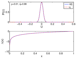
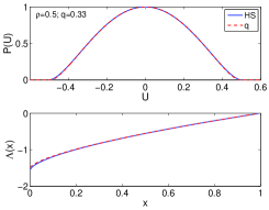
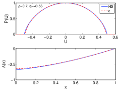
Figure 1: Top: Limit distributions al la Hilhorst-Schehr for $\rho=0.001$ (left) $0.5$ (middle), and $0.7$ (right) (lines). Broken lines are $q$-Gaussians with a $q$ from the reported best-fit value of $q=\frac{1-\frac{5}{3}\rho}{1-\rho}$, hilhorst . Bottom: Generalized logarithms necessary to provide Hilhorst-Schehr distribution functions under the maximum entropy principle (lines). Broken lines are $q$-logarithms $\ln_{q}(x)=(x^{1-q}-1)/(1-q)$ for the same $q$ values.

II Entropy for limit distributions

Let us now properly identify the distributions $P$ and ${\cal P}$ from Eqs. (8) and (17). First, note that the limit distributions in hilhorst are centered and symmetric thus the first moment does not provide any information. We therefore choose $f$ from Eq. (15) to be $f(z)=z^{2}$. Second, the one point distribution $P_{1}$ has fixed variance and so does ${\cal P}(\bar{u})$ in Eq. (8), whereas distributions obtained through the MEP Eq. (18) scale with a function of the ”inverse temperature”, $\beta$. To take this into consideration for the identification of $P$ and ${\cal P}$ we need a simple scale transformation $\bar{u}=\lambda z$, where $\lambda(\beta)$ depends explicitly on $\beta$. Consequently, ${\cal P}(\bar{u})\to\lambda{\cal P}(\lambda z)$ and

$$\lambda{\cal P}(\lambda z)=\frac{1}{\zeta}{\cal E}\left(-\alpha-\beta z^{2}\right)\quad.$$ (19)

This particular identification and the independence of Lagrange parameters requires the normalization condition $\alpha=0$ for the limit distribution Eq. (18). Further, to determine $\zeta$ and $\lambda$ we use two conditions usually valid for generalized exponential functions, ${\cal E}(0)=1$ and ${\cal E}^{\prime}(0)=1$. This leads to

$$\zeta^{-1}=\lambda\left(\frac{1-\rho}{2\pi\rho}\right)^{\frac{1}{2}}\nu_{*}^{\prime}(0)\quad{\rm and}\quad\lambda=\gamma\sqrt{\beta}\quad,$$ (20)

with $\gamma^{2}\equiv\frac{2\rho\nu_{*}^{\prime}(0)}{\nu_{*}^{\prime}(0)^{3}(1-\rho)-\nu_{*}^{\prime\prime\prime}(0)\rho}$. The generalized exponential can now be identified as

$${\cal E}\left(x\right)=\frac{\nu_{*}^{\prime}(\gamma\sqrt{-x})}{\nu_{*}^{\prime}(0)}\exp\left(-\frac{1-\rho}{2\rho}[\nu_{*}(\gamma\sqrt{-x})]^{2}\right)\quad,$$ (21)

This uniquely defines ${\cal E}$ on the domain $\left(-\infty,0\right]$. Finally, the generalized logarithm $\Lambda$ is uniquely defined on the domain $\left(0,1\right]$ as the inverse function of ${\cal E}$ and can be given explicitly for specific examples.

II.1 An example

The special case of a block function $P_{1}(u_{j})=1$ for $-\frac{1}{2}\leq u_{j}\leq\frac{1}{2}$ was discussed in hilhorst . This choice implies

$$k^{\prime}(\nu) = -\frac{\kappa e^{-\kappa^{2}\nu^{2}}}{\sqrt{\pi}}\quad,\quad\kappa\equiv\left(\frac{1-\rho}{2(2-\rho)}\right)^{\frac{1}{2}}$$

$$k(\nu) = \bar{u}-\frac{1}{2}\mbox{erf}(\kappa\nu)\quad,\quad\nu_{*}=\kappa^{-1}\mbox{erf}^{-1}(2\bar{u}),$$ (22)

and the limit distribution Eq. (8) becomes

$${\cal P}(\bar{u})=\left(\frac{2-\rho}{\rho}\right)^{\frac{1}{2}}\exp\left(-\frac{2(1-\rho)}{\rho}[\mbox{erf}^{-1}(2\bar{u})]^{2}\right)\quad.$$ (23)

This block function has been used earlier thristleton where it was conjectured on numerical evidence that the limiting distribution would be a $q$-Gaussian. This is obviously ruled out by Eq. (23), however, actual discrepancy is small, see Fig. 1. For this example Eq. (21) becomes

$${\cal E}(x)\equiv\exp\left(-(\pi\gamma^{2})^{-1}\left[\mbox{erf}^{-1}(2\gamma\sqrt{-x})\right]^{2}\right)\quad,$$ (24)

where $\gamma=\sqrt{\rho/(2\pi(1-\rho))}$. The associated generalized logarithm can be explicitly given on the domain $\left(0,1\right]$

$$\Lambda(x)=-\left[(2\gamma)^{-1}\mbox{erf}\left(\gamma\sqrt{-\pi\ln x}\right)\right]^{2}\quad.$$ (25)

It is compared to $q$-logarithms in Fig. 1; the discrepancy is small but visible.

III Discussion

Historically it was hypothesized on numerical evidence thristleton that limit distributions of sums of correlated random numbers generated along the lines of Eq. (3) might be deeply related to $q$-Gaussians, thus lending fundamental support for $q$-entropy. In hilhorst it was shown that this is not the case. If $q$-entropy does not lead to the exact limit distributions under the MEP, which form of entropy does? Here we constructively answer this question by using a recently proposed generalization of $q$-generalized entropy hanel07 , which is thermodynamically relevant abe08 . Interestingly, a similar program has been carried out some time ago for Levy stable distributions, which result from a generalized CLT where higher momenta do not exist. There it was shown that the corresponding entropy functional is Tsallis entropy abe00 , however under $q$-constraints.

Supported by Austrian Science Fund FWF Projects P17621 and P19132.

References

- (1) H.J. Hilhorst, G. Schehr, J. Stat. Mech., P06003 (2007).
- (2) F. Baldovin, A.L. Stella, Phys. Rev. E 75, 020101(R) (2007).
- (3) L.G. Moyano, C. Tsallis, M. Gell-Mann, Europhys. Lett. 73, 813-819 (2006).
- (4) S. Umarov, C. Tsallis, M. Gell-Mann, S. Steinberg, arXiv:cond-mat/0606038; cond-mat/0606040.
- (5) C. Tsallis, J. Stat. Phys. 52, 479 (1988).
- (6) G. Kaniadakis, Phys. Rev. E 66, 056125 (2002).
- (7) R. Hanel, S. Thurner, Physica A 380, 109-114 (2007).
- (8) S. Abe, S. Thurner, Europhys. Lett. 81, 10004 (2008).
- (9) W. Thistleton, J.A. Marsh, K. Nelson, C. Tsallis, arXiv:cond-mat/0605570.
- (10) S. Abe, A.K. Rajagopal, Europhys. Lett. 52, 610-614 (2000).