New formula for a resonant scattering near
an inelastic threshold

Abstract

We show that the Flatté formula is not adequate to interpret precision data on a resonance production near an inelastic threshold. A unitary parameterization, satisfying generalized Watson’s theorem for the production amplitudes, is proposed to replace the Flatté parameterization in the phenomenological analyses of the experimental data.

1 INTRODUCTION

In 1976 S. M. Flatté analysed the $\pi\eta$ and the $\rm K\overline{K}$ coupled channel systems and proposed the following parameterization of the $S$-wave production amplitudes $A_{i}$:

$$A_{i}\sim\frac{M_{R}\sqrt{\Gamma_{0}\Gamma_{i}}}{M_{R}^{2}-E^{2}-iM_{R}(\Gamma_{1}+\Gamma_{2})},~{}~{}~{}i=1,2.$$ (1)

Here $E$ is the effective mass (c.m. energy), $M_{R}$ is a resonance mass (the $a_{0}(980)$ mass in this particular case), the first channel width

$$\Gamma_{1}=g_{1}k_{1},~{}~{}~{}~{}~{}k_{1}=\frac{1}{2E}\sqrt{[E^{2}-(m_{\eta}+m_{\pi})^{2}][E^{2}-(m_{\eta}-m_{\pi})^{2}]},$$ (2)

$k_{1}$ being the pion or eta c.m. momentum. Above the $\rm K\overline{K}$ threshold the second channel width $\Gamma_{2}=g_{2}k_{2}$, where $k_{2}=\sqrt{\frac{E^{2}}{4}-m_{K}^{2}}$ is the kaon c.m. momentum. Below the threshold $\Gamma_{2}=ig_{2}p_{2}$, where $p_{2}=\sqrt{m_{K}^{2}-\frac{E^{2}}{4}}$. At the threshold energy $E_{0}=2m_{K}$, $q=k_{1}(E_{0})$ and $\Gamma_{0}=g_{1}q$. The Flatté production amplitudes (1) depend on three real parameters: the resonance mass $M_{R}$ and the two coupling constants $g_{1}$ and $g_{2}$. Some discussions related to the Flatté parameterization can be found in Refs. [2-4].

At first we consider an elastic scattering amplitude in the second channel. Without a coupling to the first channel it can be written as

$$T_{22}=\frac{\sin\delta_{2}}{k_{2}}e^{i\delta_{2}}\equiv\frac{1}{k_{2}\cot\delta_{2}-ik_{2}},$$ (3)

where $\delta_{2}$ is the channel two phase shift. Near the $\rm K\overline{K}$ threshold, for $k_{2}$ close to $0$, one gets the effective range expansion:

$$k_{2}\cot\delta_{2}\approx\frac{1}{a}+\frac{1}{2}r~{}k_{2}^{2},$$ (4)

where $a$ is the scattering length and $r$ is the effective range. Both $a$ and $r$ are real. In presence of a coupling to the first channel the $T_{22}$ amplitude (3) can to be written as

$$T_{22}=\frac{1}{2ik_{2}}(\eta e^{2i\delta_{2}}-1),$$ (5)

where $\eta$ denotes the inelasticity parameter. The inelastic coupling near the threshold can effectively be taken into account by a modification of the effective range expansion:

$$T_{22}=\frac{1}{\frac{1}{A}-i~{}k_{2}+\frac{1}{2}~{}R~{}k_{2}^{2}}.$$ (6)

Here $A$ denotes the complex scattering length and $R$ is the complex effective range. Thus for a description of the elastic scattering in the second channel one needs four real parameters. In the Flatté formula, however, we have only three parameters , so it is evident that this parameterization is not sufficient to describe a system of the two coupled channels.

We introduce a new formula for the denominator $W$ of the production amplitudes above an inelastic threshold:

$$A_{i}\sim\frac{1}{W(E)},~{}~{}~{}W(E)=M_{R}^{2}-E^{2}-iM_{R}g_{1}q-iM_{R}g_{2}k_{2}+N~{}k_{2}^{2},$$ (7)

where $N$ is a new complex constant. Below the threshold one should replace $k_{2}$ by $ip_{2}$. Since in the $\rm K\overline{K}$ channel $E^{2}=E_{0}^{2}+4k_{2}^{2}$, the denominator $W(E)$ in (7) can be directly related to the denominator of $T_{22}$ in Eq. (6):

$$\frac{W(E)}{M_{R}g_{2}}=\frac{1}{A}-ik_{2}+\frac{1}{2}Rk_{2}^{2},$$ (8)

where we find the inverse of the scattering length

$$Re(\frac{1}{A})=\frac{M_{R}^{2}-E_{0}^{2}}{M_{R}g_{2}},~{}~{}~{}Im(\frac{1}{A})=-\frac{g_{1}}{g_{2}}~{}q,$$ (9)

and the effective range

$$R=\frac{2N-8}{M_{R}g_{2}}.$$ (10)

In the Flatté approximation $N=0$, hence $ReR=\frac{-8}{M_{R}g_{2}}$ and $ImR=0$. The zero value of the imaginary part of the effective range is an essential limitation of the Flatté formula.

1.1 Elastic scattering in the first channel and a transition between channels

In close analogy to Eq. (5), the elastic scattering amplitude in the first channel depends on the phase shift $\delta_{1}$:

$$T_{11}=\frac{1}{2ik_{1}}(\eta e^{2i\delta_{1}}-1)\cdot$$ (11)

At the $\rm K\overline{K}$ threshold $\eta=1$, $\delta_{1}(q)\equiv\delta_{0}$ and $T_{11}(E_{0})=\frac{\sin\delta_{0}}{q}e^{i\delta_{0}}$. Using the unitarity property of the scattering amplitudes we can derive a new formula for $T_{11}$ above the $\rm K\overline{K}$ threshold:

$$T_{11}=\frac{e^{i\delta_{0}}}{k_{1}}\frac{\sin\delta_{0}~{}+~{}i~{}Im~{}(e^{-i\delta_{0}}~{}A)~{}k_{2}~{}-~{}\frac{1}{2}~{}Im~{}(e^{-i\delta_{0}}~{}A~{}R)~{}k_{2}^{2}}{1-~{}i~{}A~{}k_{2}~{}+~{}\frac{1}{2}~{}A~{}R~{}k_{2}^{2}}\cdot$$ (12)

There are five independent parameters in $T_{11}$: Re A, Im A, Re R, Im R and $\delta_{0}$. Below the $\rm K\overline{K}$ threshold $k_{2}\rightarrow ip_{2}$. In the Flatté limit $\delta_{0}$ equals to the phase of the complex scattering length $A$ and the second numerator of $T_{11}$ in Eq. (12) becomes constant ($\sin\delta_{0}$).

A general form of the transition amplitude from the first to the second channel is the following:

$$T_{12}=\frac{1}{2\sqrt{k_{1}k_{2}}}\sqrt{1-\eta^{2}}~{}e^{i(\delta_{1}+\delta_{2})}\cdot$$ (13)

In the new parameterization near the threshold $T_{12}$ reads:

$$T_{12}=\frac{1}{\sqrt{k_{1}}}~{}e^{i\delta_{0}}\frac{\sqrt{Im~{}A~{}-~{}\frac{1}{2}~{}|A|^{2}~{}Im~{}R~{}k_{2}^{2}}}{1-~{}i~{}A~{}k_{2}~{}+~{}\frac{1}{2}~{}A~{}R~{}k_{2}^{2}}\cdot$$ (14)

Let us remark that if $Im~{}A=Im~{}R=0$ then $T_{12}=0$ (no transition between channels). In the Flatté limit $Im~{}R=0$ and the numerator of $T_{12}$ is a constant independent on $k_{2}$.

1.2 Poles of the scattering amplitudes

All the three amplitudes, given by Eqs. (6), (12) and (14), have a common denominator

$$D(k_{2})=1-~{}i~{}A~{}k_{2}~{}+~{}\frac{1}{2}~{}A~{}R~{}k_{2}^{2}\cdot$$ (15)

The amplitude poles coincide with the zeroes of $D(k_{2})$ located at $z_{1}$ and $z_{2}$:

$$z_{1,2}=\frac{i}{R}\pm\sqrt{-\frac{1}{R^{2}}-\frac{2}{AR}}\cdot$$ (16)

From these equations we obtain the following relations for the scattering length $A$ and the effective range $R$:

$$A=-i(\frac{1}{z_{1}}+\frac{1}{z_{2}}),~{}~{}~{}~{}~{}~{}~{}~{}~{}~{}~{}~{}~{}~{}~{}~{}R=\frac{2i}{z_{1}+z_{2}}\cdot$$ (17)

In the Flatté approximation $Re~{}z_{1}~{}=-Re~{}z_{2}$. This constraint has an important impact on the values of the complex energy poles $E_{1,2}=\sqrt{E_{0}^{2}+4z_{1,2}^{2}}$.

2 New formula for the production amplitudes

Parameterization of the production amplitudes $A_{i}$ can be done in terms of the linear combination of the amplitudes $T_{ij}(k_{2})$:

$$A_{1}=f_{1}~{}T_{11}~{}+~{}f_{2}~{}T_{12},~{}~{}~{}~{}~{}A_{2}=f_{1}~{}T_{12}~{}+~{}f_{2}~{}T_{22}~{}.$$ (18)

Here $f_{1}$, $f_{2}$ are real functions of energy (or momentum $k_{2}$) and the two-channel scattering amplitudes in a new approach are written as $T_{ij}(k_{2})=\frac{N_{ij}(k_{2})}{D(k_{2})}$, where the numerators $N_{ij}$ can be directly obtained from Eqs. (12), (6) and (14) by using Eq. (15). Then

$$A_{1}=\frac{B_{1}(k_{2})}{D(k_{2})},~{}~{}~{}~{}~{}A_{2}=\frac{B_{2}(k_{2})}{D(k_{2})},$$ (19)

where

$$B_{1}=f_{1}(k_{2})N_{11}(k_{2})+f_{2}(k_{2})N_{12}(k_{2}),~{}~{}~{}~{}~{}B_{2}=f_{1}(k_{2})N_{12}(k_{2})+f_{2}(k_{2})N_{22}(k_{2})~{}.$$ (20)

A possible approximation of $f_{i}(k_{2})$ near the inelastic threshold is:

$$f_{1}(k_{2})\approx\alpha_{1}+\beta_{1}k_{2}^{2},~{}~{}~{}f_{2}(k_{2})\approx\alpha_{2}+\beta_{2}k_{2}^{2};$$ (21)

$\alpha_{1},\alpha_{2}$ are normalization constants and $\beta_{1}$,$\beta_{2}$ are real coefficients.

2.1 Watson’s theorem and its generalization above the inelastic threshold

Below the inelastic threshold Watson’s theorem is satisfied by the production amplitude $A_{1}$:

$$Im~{}A_{1}=k_{1}~{}T_{11}~{}A_{1}^{*}~{}.$$ (22)

From this equation one infers that the phase of $A_{1}$ is equal to the phase of $T_{11}$ which in turn equals to the phase shift $\delta_{1}$.

A generalization to the two coupled channels can be done as follows:

$$Im~{}A_{1}=k_{1}~{}T_{11}~{}A_{1}^{*}~{}+k_{2}~{}T_{12}~{}A_{2}^{*},$$ (23)

$$Im~{}A_{2}=k_{2}~{}T_{22}~{}A_{2}^{*}~{}+~{}k_{1}~{}T_{21}~{}A_{1}^{*}.$$ (24)

In a matrix notation one can define:

$$A=\left(\begin{array}[]{c}A_{1}\\ A_{2}\end{array}\right),~{}~{}~{}~{}~{}T=\left(\begin{array}[]{cc}T_{11}~{}~{}T_{12}\\ T_{21}~{}~{}T_{22}\end{array}\right),~{}~{}~{}~{}~{}k=\left(\begin{array}[]{cc}k_{1}~{}~{}~{}0\\ 0~{}~{}~{}k_{2}\end{array}\right)$$

and write the matrix form of the generalized Watson theorem as $Im~{}A=T~{}k~{}A^{*}$. This is equivalent to $A=S~{}A^{*}$, where $S$ denotes the $S-$ matrix. Its elements are related to the scattering matrix elements $T_{ij}$ ($i,j=1,2$) by

$$S_{ij}=\delta_{ij}+2~{}i~{}\sqrt{k_{i}k_{j}}~{}T_{ij}~{}.$$ (25)

3 Numerical example: a case of the $a_{0}(980)$ resonance

The $a_{0}(980)$ resonance is situated close to the $\rm K\overline{K}$ threshold. It decays predominantly to the $\pi\eta$ channel in which two mesons interact in the $S$-wave, isospin one state. A coupled channel formalism for the separable meson-meson interactions in two or three channels has been developed in LL . Then in Ref. AFLL it was applied to study the $a_{0}$ resonances in the $\pi\eta$ and the $\rm K\overline{K}$ channels. The model parameters were fixed using the data of the Crystal Barrel and of the E-852 Collaborations. The following threshold parameters have been presently calculated: $Re~{}A=0.17$ fm, $Im~{}A=0.41$ fm, $Re~{}R=-11.32$ fm, and $Im~{}R=-3.18$ fm. Let us stress here that the imaginary part of the effective range cannot be neglected. In Fig. 1 we see important differences between the amplitude intensities calculated in two cases: 1. for $Im~{}R=-3.18$ fm and 2. $Im~{}R=0$ fm (Flatté’s limit). All curves are normalized to 1 at the $\rm K\overline{K}$ threshold but already at the distance of 50 MeV to the left and to the right of the maximum the relative deviations between the two cases reach as much as 100 %.

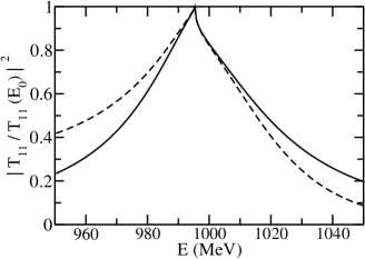
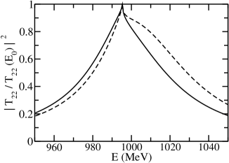
Figure 1: Squares of the amplitude moduli versus the c.m. energy. The solid lines correspond to the new parameterization, given by Eqs. (6) and (12), the dashed lines - to the Flatté formula.

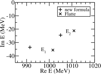
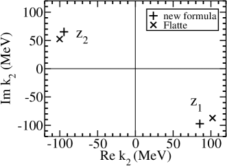
Figure 2: Pole positions in the $\rm K\overline{K}$ complex energy plane (left panel) and in the complex momentum plane (right panel)

In Fig. 2 the pole positions of the amplitudes are shown in the complex momentum $k_{2}$ and in the complex energy planes. One can notice a large shift of $Re~{}E_{1}$ between the new result and the Flatté value. It exceeds 10 MeV and is larger than the present experimental energy resolution of many experiments. Thus, using the Flatté formula in the data analysis can lead to an important distortion of the particle spectra and to large theoretical errors of the threshold parameters. In particular, this may influence resonance masses and widths presented by the Particle Data Group in the Review of Particle Physics. The phases of the scattering amplitudes are also different in the two cases.

4 CONCLUSIONS

1. The Flatté formula is not sufficiently accurate to be used in analyses of the newest data on the resonance production near inelastic thresholds. Its application can lead to a substantial distortion of the effective mass distributions and to a displacement of the resonance pole positions.

2. A simple unitary parameterization, satisfying a generalized Watson theorem for the production amplitudes, is proposed. It enables one to determine crucial measurable particle interaction parameters, like the complex scattering length and the complex effective range. It is shown that a near threshold resonance should be characterized by two distinct complex poles.

3. A generalization of the new parameterization to the coupled particle systems other than $\pi\eta$ and $\rm K\overline{K}$ is straightforward.

4. New formula can be applied in numerous analyses of present and future experiments (for example: Belle, BaBar, CLEO, BES, KLOE, COSY, Tevatron, LHC, CLAS at JLab, Panda etc.). They can also serve to reanalyse older experiments with an aim to improve our knowledge of hadron spectroscopy and of reaction mechanisms.

References

(1)
S. M. Flatté, Phys. Lett., B63, 224 (1976).
(2)
V. Baru, J. Heidenbauer, C. Hahnhart, Yu. Kalashnikova, A. Kudryavtsev,
Phys. Lett., B586, 53 (2004).
(3)
B. Kerbikov, Phys. Lett., B596, 200 (2004).
(4)
V. Baru, J. Heidenbauer, C. Hahnhart, A. Kudryavtsev, U.-G. Meissner,
Eur. Phys. J., A23, 523 (2005)
(5)
L. Leśniak, Acta Physica Polonica, B27, 1835 (1996).
(6)
Agnieszka Furman and Leonard Leśniak, Phys. Lett., B538, 266 (2002).