Natural pseudo-distance and optimal matching between reduced size functions

Abstract

This paper studies the properties of a new lower bound for the natural pseudo-distance. The natural pseudo-distance is a dissimilarity measure between shapes, where a shape is viewed as a topological space endowed with a real-valued continuous function. Measuring dissimilarity amounts to minimizing the change in the functions due to the application of homeomorphisms between topological spaces, with respect to the $L_{\infty}$-norm. In order to obtain the lower bound, a suitable metric between size functions, called matching distance, is introduced. It compares size functions by solving an optimal matching problem between countable point sets. The matching distance is shown to be resistant to perturbations, implying that it is always smaller than the natural pseudo-distance. We also prove that the lower bound so obtained is sharp and cannot be improved by any other distance between size functions.

1 Introduction

Shape comparison is a fundamental problem in shape recognition, shape classification and shape retrieval (cf., e.g., [24]), finding its applications mainly in Computer Vision and Computer Graphics. The shape comparison problem is often dealt with by defining a suitable distance providing a measure of dissimilarity between shapes (see, e.g., [25] for a review of the literature).

Over the last fifteen years, Size Theory has been developed as a geometrical-topological theory for comparing shapes, each shape viewed as a topological space $\mathcal{M}$, endowed with a real-valued continuous function $\varphi$ [15]. The pair $(\mathcal{M},\varphi)$ is called a size pair, while $\varphi$ is said to be a measuring function. The role of the function $\varphi$ is to take into account only the shape properties of the object described by $\mathcal{M}$ that are relevant to the shape comparison problem at hand, while disregarding the irrelevant ones, as well as to impose the desired invariance properties.

A measure of the dissimilarity between two size pairs is given by the natural pseudo-distance. The main idea in the definition of natural pseudo-distance between size pairs is to minimize the change in the measuring functions due to the application of homeomorphisms between topological spaces, with respect to the $L_{\infty}$-norm: The natural pseudo-distance between $(\mathcal{M},\varphi)$ and $(\mathcal{N},\psi)$ with $\mathcal{M}$ and $\mathcal{N}$ homeomorphic is the number

$$\inf_{h}\max_{P\in\mathcal{M}}|\varphi(P)-\psi(h(P))|,$$

where $h$ varies in the set $H(\mathcal{M},\mathcal{N})$ of all the homeomorphisms between $\mathcal{M}$ and $\mathcal{N}$. In other words, the variation of the shapes is modeled by the infinite-dimensional group of homeomorphisms and the cost of warping an object’s shape into another is measured by the change of the measuring functions. An important feature of the natural pseudo-distance is that it does not require the choice of parametrizations for the spaces under study nor the choice of origins of coordinate, which in image applications would be arbitrarily driven.

The main aim of this paper is to provide a new method to estimate the natural pseudo-distance, motivated by the intrinsic difficulty of a direct computation. Since the natural pseudo-distance is defined by a minimization process, it would be natural to look for the optimal transformation that takes one shape into the other, as usual in energy minimization methods. In our case, however, the existence of an optimal homeomorphism attaining the natural pseudo-distance is not guaranteed.

Earlier results about the natural pseudo-distance can be divided in two classes. One class provides constraints on the possible values taken by the natural pseudo-distance between two size pairs. For example, if the considered topological spaces $\mathcal{M}$ and $\mathcal{N}$ are smooth closed manifolds and the measuring functions are also smooth, then the natural pseudo-distance is an integer sub-multiple of the Euclidean distance between two suitable critical values of the measuring functions [8]. In particular, this integer can only be either $1$ or $2$ in the case of curves, while it can be either $1$, $2$ or $3$ in the case of surfaces [9]. The other class of results furnishes lower bounds for the natural pseudo-distance [7], [18]. In particular it is possible to estimate the natural pseudo-distance by using the concept of size function [7]. Indeed, size functions can reduce the comparison of shapes to the comparison of certain countable subsets of the real plane (cf. [10], [13] and [16]). This reduction allows us to study the space of all homeomorphisms between the considered topological spaces, without actually computing them. The research on size functions has led to a formal setting, which has turned out to be useful, not only from a theoretical point of view, but also on the applicative side (see, e.g., [1], [3], [5], [6], [14], [19], [21]).

This paper investigates into the problem of obtaining lower bounds for the natural pseudo-distance using size functions.

To this aim, we first introduce the concept of reduced size function. Reduced size functions are a slightly modified version of size functions based on the connectedness relation instead of path-connectedness. This new definition is introduced in order to obtain both theoretical and computational advantages (see Rem. 3 and Rem. 9). However, the main properties of size functions are maintained. In particular, reduced size functions can be represented by sets of points of the (extended) real plane, called cornerpoints.

Then we need a preliminary result about reduced size functions (Th. 25). It states that a suitable distance between reduced size functions exists, which is continuous with respect to the measuring functions (in the sense of the $L_{\infty}$-topology). We call this distance matching distance, since the underlying idea is to measure the cost of matching the two sets of cornerpoints describing the reduced size functions. The matching distance reduces to the bottleneck distance used in [4] for comparing Persistent Homology Groups when the measuring functions are taken in the subset of tame functions. We underline that the continuity of the matching distance implies a property of perturbation robustness for size functions allowing them to be used in real applications.

Having proven this, we are ready to obtain our main results. Indeed, the stability of the matching distance allows us to prove a sharp lower bound for the change of measuring functions under the action of homeomorphisms between topological spaces, i.e. for the natural pseudo-distance (Th. 29). Furthermore, we prove that the lower bound obtained using the matching distance not only improves the previous known lower bound stated in [7], but is the best possible lower bound for the natural pseudo-distance obtainable using size functions. The proof of these facts is based on Lemma 30. This lemma is a crucial result stating that it is always possible to construct two suitable measuring functions on a topological $2$-sphere with given reduced size functions and a pseudo-distance equaling their matching distance. On the basis of this lemma, in Th. 32 and Th. 34 we prove that the matching distance we are considering is, in two different ways, the best metric to compare reduced size functions.

This paper is organized as follows. In Section 2 we introduce the concept of reduced size function and its main properties. In Section 3 the definition of matching distance between reduced size functions is given. In Section 4 the stability theorem is proved, together with some other useful results. The connection with natural pseudo-distances between size pairs is shown in Section 5, together with the proof of the existence of an optimal matching between reduced size functions. Section 6 contains the proof that it is always possible to construct two size pairs with pre-assigned reduced size functions and a pseudo-distance equaling their matching distance. This result is used in Section 7 to conclude that the matching distance furnishes the finest lower bound for the natural pseudo-distance between size pairs among the lower bounds obtainable through reduced size functions. In Section 8 our results are briefly discussed.

2 Reduced size functions

In this section we introduce reduced size functions, that is, a notion derived from size functions ([15]) allowing for a simplified treatment of the theory. The definition of reduced size function differs from that of size function in that it is based on the relation of connectedness rather than on path-connectedness. The motivation for this change, as explained in Remark 3, has to do with the right-continuity of size functions.

In what follows, $\mathcal{M}$ denotes a non-empty compact connected and locally connected Hausdorff space, representing the object whose shape is under study.

The assumption on the connectedness of $\mathcal{M}$ can easily be weakened to any finite number of connected components without much affecting the following results. More serious problems would derive from considering an infinite number of connected components.

We shall call any pair $(\mathcal{M},\varphi)$, where $\varphi:\mathcal{M}\rightarrow\mathbb{R}$ is a continuous function, a size pair. The function $\varphi$ is said to be a measuring function. The role of the function $\varphi$ is to take into account only the shape properties of the object described by $\mathcal{M}$ that are relevant to the shape comparison problem at hand, while disregarding the irrelevant ones, as well as to impose the desired invariance properties.

Assume a size pair $({\mathcal{M}},\varphi)$ is given. For every $x\in\mathbb{R}$, let ${\mathcal{M}}\langle\varphi\leq x\rangle$ denote the lower level set $\{P\in{\mathcal{M}}:\varphi(P)\leq x\}$.

Definition 1

For every real number $y$, we shall say that two points $P,Q\in{\mathcal{M}}$ are $\langle\varphi\leq y\rangle$-connected if and only if a connected subset $C$ of ${\mathcal{M}}\langle\varphi\leq y\rangle$ exists, containing both $P$ and $Q$.

In the following, $\Delta$ denotes the diagonal $\{(x,y)\in\mathbb{R}^{2}:x=y\}$; $\Delta^{+}$ denotes the open half-plane $\{(x,y)\in\mathbb{R}^{2}:x<y\}$ above the diagonal; ${\bar{\Delta}^{+}}$ denotes the closed half-plane $\{(x,y)\in\mathbb{R}^{2}:x\leq y\}$ above the diagonal.

Definition 2

(Reduced size function) We shall call reduced size function associated with the size pair $(\mathcal{M},\varphi)$ the function ${\ell^{*}_{(\mathcal{M},\varphi)}}:\Delta^{+}\rightarrow\mathbb{N}$, defined by setting $\ell^{*}_{({\mathcal{M}},\varphi)}(x,y)$ equal to the number of equivalence classes into which the set ${\mathcal{M}}\langle\varphi\leq x\rangle$ is divided by the relation of $\langle\varphi\leq y\rangle$-connectedness.

In other words, $\ell^{*}_{({\mathcal{M}},\varphi)}(x,y)$ counts the number of connected components in ${\mathcal{M}}\langle\varphi\leq y\rangle$ that contain at least one point of ${\mathcal{M}}\langle\varphi\leq x\rangle$. The finiteness of this number is an easily obtainable consequence of the compactness and local-connectedness of $\mathcal{M}$.

\psfrag{P}{$P$}\psfrag{a}{$a$}\psfrag{b}{$b$}\psfrag{c}{$c$}\psfrag{e}{$e$}\psfrag{x}{$x$}\psfrag{y}{$y$}\psfrag{0}{$0$}\psfrag{1}{$1$}\psfrag{2}{$2$}\psfrag{3}{$3$}\includegraphics[width=289.07999pt]{sf.eps}

Figure 1: (b) The reduced size function of the size pair $(\mathcal{M},\varphi)$, where $\mathcal{M}$ is the curve represented by a continuous line in (a), and $\varphi$ is the function “distance from the point $P$”.

An example of reduced size function is illustrated in Fig. 1. In this example we consider the size pair $(\mathcal{M},\varphi)$, where $\mathcal{M}$ is the curve represented by a continuous line in Fig. 1 (a), and $\varphi$ is the function “distance from the point $P$”. The reduced size function associated with $(\mathcal{M},\varphi)$ is shown in Fig. 1 (b). Here, the domain of the reduced size function is divided by solid lines, representing the discontinuity points of the reduced size function. These discontinuity points divide $\Delta^{+}$ into regions in which the reduced size function is constant. The value displayed in each region is the value taken by the reduced size function in that region.

For instance, for $a\leq x<b$, the set $\{P\in\mathcal{M}:\varphi(P)\leq x\}$ has two connected components which are contained in different connected components of $\{P\in\mathcal{M}:\varphi(P)\leq y\}$ when $x<y<b$. Therefore, $\ell^{*}_{\left({\mathcal{M}},\varphi\right)}(x,y)=2$ for $a\leq x<b$ and $x<y<b$. When $a\leq x<b$ and $y\geq b$, all the connected components of $\{P\in\mathcal{M}:\varphi(P)\leq x\}$ are contained in the same connected component of $\{P\in\mathcal{M}:\varphi(P)\leq y\}$. Therefore, $\ell^{*}_{\left({\mathcal{M}},\varphi\right)}(x,y)=1$ for $a\leq x<b$ and $y\geq b$. When $b\leq x<c$ and $y\geq c$, all of the three connected components of $\{P\in\mathcal{M}:\varphi(P)\leq x\}$ belong to the same connected component of $\{P\in\mathcal{M}:\varphi(P)\leq y\}$, implying that in this case $\ell^{*}_{\left({\mathcal{M}},\varphi\right)}(x,y)=1$.

As for the values taken on the discontinuity lines, they are easily obtained by observing that reduced size functions are right-continuous, both in the variable $x$ and in the variable $y$.

Remark 3

The property of right-continuity in the variable $x$ can easily be checked and holds for classical size functions as well. The analogous property for the variable $y$ is not immediate, and in general does not hold for classical size functions, if not under stronger assumptions, such as, for instance, that $\mathcal{M}$ is a smooth manifold and the measuring function is Morse (cf. Cor. 2.1 in [12]). Indeed, the relation of $\langle\varphi\leq y\rangle$-homotopy, used to define classical size functions, does not pass to the limit. On the contrary, the relation of $\langle\varphi\leq y\rangle$-connectedness does, that is to say, if, for every $\epsilon>0$ it holds that $P$ and $Q$ are $\langle\varphi\leq y+\epsilon\rangle$-connected, then they are $\langle\varphi\leq y\rangle$-connected. To see this, observe that connected components are closed sets, and the intersection $\bigcap_{i}K_{i}$ of a family of compact, connected Hausdorff subspaces $K_{i}$ of a topological space, with the property that $K_{i+1}\subseteq K_{i}$ for every $i$, is connected (cf. Th. 28.2 in [26] p. 203).

Most properties of classical size functions continue to hold for reduced size functions. For the aims of this paper, it is important that for reduced size functions it is possible to define an analog of classical size functions’ cornerpoints and cornerlines, here respectively called proper cornerpoints and cornerpoints at infinity. The main reference here is [16].

Definition 4

(Proper cornerpoint) For every point $p=(x,y)\in\Delta^{+}$, let us define the number $\mu(p)$ as the minimum over all the positive real numbers $\epsilon$, with $x+\epsilon<y-\epsilon$, of

$$\ell^{*}_{({\mathcal{M}},\varphi)}(x+\epsilon,y-\epsilon)-\ell^{*}_{({\mathcal{M}},\varphi)}(x-\epsilon,y-\epsilon)-\ell^{*}_{({\mathcal{M}},\varphi)}(x+\epsilon,y+\epsilon)+\ell^{*}_{({\mathcal{M}},\varphi)}(x-\epsilon,y+\epsilon).$$

The finite number $\mu(p)$ will be called multiplicity of $p$ for $\ell^{*}_{({\mathcal{M}},\varphi)}$. Moreover, we shall call proper cornerpoint for $\ell^{*}_{({\mathcal{M}},\varphi)}$ any point $p\in\Delta^{+}$ such that the number $\mu(p)$ is strictly positive.

Definition 5

(Cornerpoint at infinity) For every vertical line $r$, with equation $x=k$, let us identify $r$ with the pair $(k,\infty)$, and define the number $\mu(r)$ as the minimum, over all the positive real numbers $\epsilon$ with $k+\epsilon<1/\epsilon$, of

$$\ell^{*}_{({\mathcal{M}},\varphi)}(k+\epsilon,1/\epsilon)-\ell^{*}_{({\mathcal{M}},\varphi)}(k-\epsilon,1/\epsilon).$$

When this finite number, called multiplicity of $r$ for $\ell^{*}_{({\mathcal{M}},\varphi)}$, is strictly positive, we call the line $r$ a cornerpoint at infinity for the reduced size function.

Remark 6

The multiplicity of points and of vertical lines is always non negative. This follows from an analog of Lemma 1 in [16], based on counting the equivalence classes in the set

$$\left\{P\in{\mathcal{M}}\langle\varphi\leq x_{2}\rangle:\not\!\exists Q\in{M}\langle\varphi\leq x_{1}\rangle\ s.t.\ P\cong_{\varphi\leq y_{1}}Q\right\}$$

quotiented by the relation of $\langle\varphi\leq y_{1}\rangle$-connectedness, in order to obtain the number

$${\ell^{*}_{(\mathcal{M},\varphi)}}(x_{2},y_{1})-{\ell^{*}_{(\mathcal{M},\varphi)}}(x_{1},y_{1})$$

when $x_{1}\leq x_{2}<y_{1}$.

Remark 7

Under our assumptions on $\mathcal{M}$, i.e. its connectedness, $\mu(r)$ can only take the values $0$ and $1$, but the definition can easily be extended to spaces with any finite number of connected components, so that $\mu(r)$ can equal any natural number. Moreover, the connectedness assumption also implies that there is exactly one cornerpoint at infinity.

As an example of cornerpoints in reduced size functions, in Fig. 2 we see that the proper cornerpoints are the points $p$, $q$ and $r$ (with multiplicity $2$, $1$ and $1$, respectively). The line $m$ is the only cornerpoint at infinity.

\psfrag{x}{$x$}\psfrag{y}{$y$}\psfrag{m}{$m$}\psfrag{p}{$p$}\psfrag{q}{$q$}\psfrag{s}{$s$}\psfrag{r}{$r$}\psfrag{0}{$0$}\psfrag{1}{$1$}\psfrag{3}{$3$}\psfrag{4}{$4$}\psfrag{6}{$6$}\psfrag{7}{$7$}\psfrag{5}{$5$}\includegraphics[width=144.54pt]{value.eps}

Figure 2: Cornerpoints of a reduced size function: in this example, $p$, $q$ and $r$ are the only proper cornerpoints, and have multiplicity equal to $2$ ($p$) and $1$ ($r,q$). The point $s$ is not a cornerpoint, since its multiplicity vanishes. The line $m$ is the only cornerpoint at infinity.

The importance of cornerpoints is revealed by the next result, analogous to Prop. 10 of [16], showing that cornerpoints, with their multiplicities, uniquely determine reduced size functions.

The open (resp. closed) half-plane $\Delta^{+}$ (resp. $\bar{\Delta}^{+}$) extended by the points at infinity of the kind $(k,\infty)$ will be denoted by $\Delta^{*}$ (resp. $\bar{\Delta}^{*}$), i.e.

$$\Delta^{*}:=\Delta^{+}\cup\{(k,\infty):k\in\mathbb{R}\},\ \ \bar{\Delta}^{*}:=\bar{\Delta}^{+}\cup\{(k,\infty):k\in\mathbb{R}\}.$$

Theorem 8

(Representation Theorem) For every $({\bar{x}},{\bar{y}})\in\Delta^{+}$ we have

$$\ell^{*}_{({\mathcal{M}},\varphi)}({\bar{x}},{\bar{y}})=\sum_{(x,y)\in\Delta^{*}\atop x\leq{\bar{x}},y>\bar{y}}\mu\big{(}(x,y)\big{)}.$$ (1)

The equality (1) can be checked in the example of Fig. 2. The points where the reduced size function takes value $0$ are exactly those for which there is no cornerpoint (either proper or at infinity) lying to the left and above them. Let us take a point in the region of the domain where the reduced size function takes the value $3$. According to the above theorem, the value of the reduced size function at that point must be equal to $\mu(m)+\mu(p)=3$.

Remark 9

By comparing Th. 8 and the analogous result stated in Prop. 10 of [16], one can observe that the former is stated more straightforwardly. As a consequence of this simplification, all the statements in this paper that follow from Th. 8 are less cumbersome than they would be if we applied size functions instead of reduced size functions. This is the main motivation for introducing the notion of reduced size function.

In order to make this paper self-contained, in the rest of this section we report all and only those results about size functions that will be needed for proving our statements in the next sections, re-stating them in terms of reduced size functions. Proofs are omitted, since they are completely analogous to those for classical size functions.

The following result, expressing a relation between two reduced size functions corresponding to two spaces, $\mathcal{M}$ and $\mathcal{N}$, that can be matched without changing the measuring functions more that $h$, is analogous to Th. 3.2 in [14].

Proposition 10

Let $(\mathcal{M},\varphi)$ and $(\mathcal{N},\psi)$ be two size pairs. If $f:\mathcal{M}\rightarrow\mathcal{N}$ is a homeomorphism such that $\max_{P\in\mathcal{M}}|\varphi(P)-\psi(f(P))|\leq h$, then for every $({\bar{x}},{\bar{y}})\in\Delta^{+}$ we have

$${\ell^{*}_{(\mathcal{M},\varphi)}}({\bar{x}}-h,{\bar{y}}+h)\leq{\ell^{*}_{(\mathcal{N},\psi)}}({\bar{x}},{\bar{y}}).$$

The next proposition, analogous to Prop. 6 in [16], gives some constraints on the presence of discontinuity points for reduced size functions.

Proposition 11

Let $(\mathcal{M},\varphi)$ be a size pair. For every point ${\bar{p}}=({\bar{x}},{\bar{y}})\in\Delta^{+}$, a real number $\epsilon>0$ exists such that the open set

$$W_{\epsilon}({\bar{p}}):=\{(x,y)\in\mathbb{R}^{2}:|{\bar{x}}-x|<\epsilon,|{\bar{y}}-y|<\epsilon,x\neq{\bar{x}},y\neq{\bar{y}}\}$$

is contained in $\Delta^{+}$, and does not contain any discontinuity point for ${\ell^{*}_{(\mathcal{M},\varphi)}}$.

The following analog of Prop. 8 and Cor. 4 in [16], stating that cornerpoints create discontinuity points spreading downwards and towards the right to $\Delta$, also holds for reduced size functions.

Proposition 12

(Propagation of discontinuities) If ${\bar{p}}=({\bar{x}},{\bar{y}})$ is a proper cornerpoint for ${\ell^{*}_{(\mathcal{M},\varphi)}}$, then the following statements hold:

i) If ${\bar{x}}\leq x<{\bar{y}}$, then ${\bar{y}}$ is a discontinuity point for ${\ell^{*}_{(\mathcal{M},\varphi)}}(x,\cdot)$;

ii) If ${\bar{x}}<y<{\bar{y}}$, then ${\bar{x}}$ is a discontinuity point for ${\ell^{*}_{(\mathcal{M},\varphi)}}(\cdot,y)$.

If ${\bar{r}}=({\bar{x}},{\infty})$ is the cornerpoint at infinity for ${\ell^{*}_{(\mathcal{M},\varphi)}}$, then the following statement holds:

iii) If ${\bar{x}}<y$, then ${\bar{x}}$ is a discontinuity point for ${\ell^{*}_{(\mathcal{M},\varphi)}}(\cdot,y)$.

The position of cornerpoints in $\Delta^{+}$ is related to the extrema of the measuring function as the next proposition states, immediately following from the definitions.

Proposition 13

(Localization of cornerpoints) If ${\bar{p}}=({\bar{x}},{\bar{y}})$ is a proper cornerpoint for ${\ell^{*}_{(\mathcal{M},\varphi)}}$, then

$$\bar{p}\in\{(x,y)\in\mathbb{R}^{2}:\min\varphi\leq x<y\leq\max\varphi\}.$$

If ${\bar{r}}=({\bar{x}},\infty)$ is the cornerpoint at infinity for ${\ell^{*}_{(\mathcal{M},\varphi)}}$, then $\bar{x}=\min\varphi$.

Prop. 12 and Prop. 13 imply that the number of cornerpoints is either finite or countably infinite. In fact, the following result can be proved, analogous to Cor. 3 in [16].

Proposition 14

(Local finiteness of cornerpoints) For each strictly positive real number $\epsilon$, reduced size functions have, at most, a finite number of cornerpoints in $\{(x,y)\in\mathbb{R}^{2}:x+\epsilon<y\}$.

\psfrag{x}{$x$}\psfrag{y}{$y$}\psfrag{p}{$\varphi$}\includegraphics[height=142.26378pt]{accumul.eps}

Figure 3: A reduced size function with cornerpoints accumulating onto the diagonal: $\mathcal{M}$ is the space depicted on the left and $\varphi$ measures the height of each point.

Therefore, if the set of cornerpoints of a reduced size function has an accumulation point, it necessarily belongs to the diagonal $\Delta$. An example of reduced size function with cornerpoints accumulating onto the diagonal is shown in Fig. 3.

Moreover, this last proposition implies that in the summation of Th. 8 (Representation Theorem), only finitely many terms are different from zero.

3 Matching distance

In this section we define a matching distance between reduced size functions. The idea is to compare reduced size functions by measuring the cost of transporting the cornerpoints of one reduced size function to those of the other one, with the property that the longest of the transportations should be as short as possible. Since, in general, the number of cornerpoints of the two reduced size functions is different, we also enable the cornerpoints to be transported onto the points of $\Delta$ (in other words, we can “destroy” them).

When the number of cornerpoints is finite, the matching distance may be related to the bottleneck transportation problem (cf., e.g., [11], [20]). In our case, however, the number of cornerpoints may be countably infinite, because of our loose assumption on the measuring function, that is only required to be continuous. Nevertheless, we prove the existence of an optimal matching. Under more tight assumptions on the measuring function, the number of cornerpoints is ensured to be finite and a bottleneck distance can be more straightforwardly defined. For example, in [4] a bottleneck distance for comparing Persistent Homology Groups is introduced under the assumption that the measuring functions are tame. We recall that a continuous function is tame if it has a finite number of homological critical values and the homology groups of the lower level sets it defines are finite dimensional.

Although working with measuring functions that are continuous rather than tame involves working in an infinite dimensional space, yielding many technical difficulties in the proof of our results (for instance, compare our Matching Stability Theorem 25 with the analogous Bottleneck Stability Theorem for Persistence Diagrams in [4]), there are strong motivations for doing so. First of all, in real applications noise cannot be assumed to be tame, so that the perturbation of a tame function may happen to be not tame. In second place, when working in the more general setting of measuring functions with values in ${\mathbb{R}}^{k}$ instead of ${\mathbb{R}}$, it is important that the set of functions is closed under the action of the $\max$ operator, as shown in [2], whereas the set of tame functions is not. Last but not least, working with continuous functions allows us to relate the matching distance to the natural pseudo-distance, which is our final goal, without restricting the set of homeomorphism to those preserving the tameness property.

Of course the matching distance is not the only metric between reduced size functions that we could think of. Other metrics for size functions have been considered in the past ([10], [13]). However, the matching distance is of particular interest since, as we shall see, it allows for a connection with the natural pseudo-distance between size pairs, furnishing the best possible lower bound. Moreover, it has already been experimentally tested successfully in [1] and [3].

In order to introduce the matching distance between reduced size functions we need some new definitions. The following definition of representative sequence is introduced in order to manage the presence in a size function of infinitely many cornerpoints as well as that of their multiplicities. Moreover, it allows us to add to the set of cornerpoints a subset of points of the diagonal.

Definition 15

(Representative sequence) Let $\ell^{*}$ be a reduced size function. We shall call representative sequence for $\ell^{*}$ any sequence of points $a:\mathbb{N}\rightarrow{\bar{\Delta}^{*}}$, (briefly denoted by $(a_{i})$), with the following properties:

1. $a_{0}$ is the cornerpoint at infinity for $\ell^{*}$;

2. For each $i>0$, either $a_{i}$ is a proper cornerpoint for $\ell^{*}$, or $a_{i}$ belongs to $\Delta$;

3. If $p$ is a proper cornerpoint for $\ell^{*}$ with multiplicity $\mu(p)$, then the cardinality of the set $\{i\in\mathbb{N}:a_{i}=p\}$ is equal to $\mu(p)$;

4. The set of indexes for which $a_{i}$ is in $\Delta$ is countably infinite.

We now consider the following pseudo-distance $d$ on $\bar{\Delta}^{*}$ in order to assign a cost to each deformation of reduced size functions:

$$d\left(\left(x,y\right),\left(x^{\prime},y^{\prime}\right)\right):=\min\left\{\max\left\{|x-x^{\prime}|,|y-y^{\prime}|\right\},\max\left\{\frac{y-x}{2},\frac{y^{\prime}-x^{\prime}}{2}\right\}\right\},$$

with the convention about $\infty$ that $\infty-y=y-\infty=\infty$ for $y\neq\infty$, $\infty-\infty=0$, $\frac{\infty}{2}=\infty$, $|\infty|=\infty$, $\min\{\infty,c\}=c$, $\max\{\infty,c\}=\infty$.

In other words, the pseudo-distance $d$ between two points $p$ and $p^{\prime}$ compares the cost of moving $p$ to $p^{\prime}$ and the cost of moving $p$ and $p^{\prime}$ onto the diagonal and takes the smaller. Costs are computed using the distance induced by the $\max$-norm. In particular, the pseudo-distance $d$ between two points $p$ and $p^{\prime}$ on the diagonal is always $0$; the pseudo-distance $d$ between two points $p$ and $p^{\prime}$, with $p$ above the diagonal and $p^{\prime}$ on the diagonal, is equal to the distance, induced by the $\max$-norm, between $p$ and the diagonal. Points at infinity have a finite distance only to other points at infinity, and their distance depends on their abscissas.

Therefore, $d(p,p^{\prime})$ can be considered a measure of the minimum of the costs of moving $p$ to $p^{\prime}$ along two different paths (i.e. the path that takes $p$ directly to $p^{\prime}$ and the path that passes through $\Delta$). This observation easily yields that $d$ is actually a pseudo-distance.

Remark 16

It is useful to observe what disks induced by the pseudo-distance $d$ look like. For $r>0$, the usual notation $B(p,r)$ will denote the open disk $\{p^{\prime}\in\bar{\Delta}^{+}:d(p,p^{\prime})<r\}$. Thus, if $p$ is a proper point with coordinates $(x,y)$ and $y-x\geq 2r$ (that is, $d(p,\Delta)\geq r$), then $B(p,r)$ is the open square centered at $p$ with sides of length $2r$ parallel to the axes. Whereas, if $p$ has coordinates $(x,y)$ with $y-x<2r$ (that is, $d(p,\Delta)<r$), then $B(p,r)$ is the union of the open square, centered at $p$, with sides of length $2r$ parallel to the axes, with the stripe $\{(x,y)\in\mathbb{R}^{2}:0\leq y-x<2r\}$, intersected with $\bar{\Delta}^{+}$(see also Fig. 4). If $p=(x,\infty)$ is a point at infinity then $B(p,r)=\{(x^{\prime},\infty)\in\Delta^{*}:|x-x^{\prime}|<r\}$.

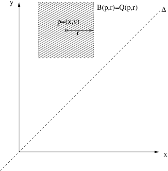
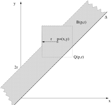
Figure 4: Disks induced by the pseudo-metric $d$ (shaded). Left: $d(p,\Delta)\geq r$. Right: $d(p,\Delta)<r$.

In what follows, the notation $Q(p,r)$ will refer to the open square centered at the proper point $p$, with sides of length $2r$ parallel to the axes (that is, the open disk centered at $p$ with radius $r$, induced by the $\max$-norm). Also, when $r>0$, ${\bar{Q}}(p,r)$ will refer to the closure of $Q(p,r)$ in the usual Euclidean topology, while ${\bar{Q}}(p,0):=\{p\}$.

Definition 17

(Matching distance) Let $\ell^{*}_{1}$ and $\ell^{*}_{2}$ be two reduced size functions. If $(a_{i})$ and $(b_{i})$ are two representative sequences for $\ell^{*}_{1}$ and $\ell^{*}_{2}$ respectively, then the matching distance between $\ell^{*}_{1}$ and $\ell^{*}_{2}$ is the number

$$d_{match}(\ell^{*}_{1},\ell^{*}_{2}):=\inf_{\sigma}\sup_{i}d(a_{i},b_{\sigma(i)}),$$

where $i$ varies in $\mathbb{N}$ and $\sigma$ varies among all the bijections from $\mathbb{N}$ to $\mathbb{N}$.

In order to illustrate this definition, let us consider Fig. 5. Given two curves, their reduced size functions with respect to the measuring function distance from the center of the image are calculated. One sees that the top reduced size function has many cornerpoints close to the diagonal in addition to the cornerpoints $r$, $a$, $b$, $c$, $d$, $e$. Analogously, the bottom reduced size function has many cornerpoints close to the diagonal in addition to the cornerpoints $r^{\prime}$, $a^{\prime}$, $b^{\prime}$, $c^{\prime}$. Cornerpoints close to the diagonal are generated by noise and discretization. The superimposition of the two reduced size functions shows that an optimal matching is given by $r\to r^{\prime}$, $a\to a^{\prime}$, $b\to b^{\prime}$, $c\to c^{\prime}$, $d\to\Delta$, $e\to\Delta$, and all the other cornerpoints sent to $\Delta$. Sending cornerpoints to points of $\Delta$ corresponds to the annihilation of cornerpoints. Since the matching $c\to c^{\prime}$ is the one that achieves the maximum cost in the $\max$-norm, the matching distance is equal to the distance between $c$ and $c^{\prime}$ (with respect to the $\max$-norm).

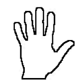
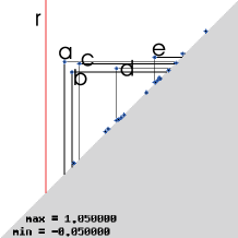
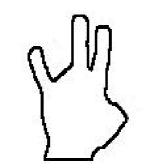
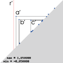
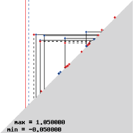
Figure 5: Left: Two curves. Center: Their reduced size functions with respect to the measuring function distance from the center of the image. Right: The superimposition of the two reduced size functions.

Proposition 18

$d_{match}$ is a distance between reduced size functions.

[Proof.] It is easy to see that this definition is independent from the choice of the representative sequences of points for $\ell^{*}_{1}$ and $\ell^{*}_{2}$. In fact, if $(a_{i})$ and $({\hat{a}}_{i})$ are representative sequences for the same reduced size function $\ell^{*}$, a bijection $\hat{\sigma}:\mathbb{N}\rightarrow\mathbb{N}$ exists such that $d({\hat{a}}_{i},a_{{\hat{\sigma}}(i)})=0$ for every index $i$.

Furthermore, we have that $d_{match}({\ell^{*}_{(\mathcal{M},\varphi)}},{\ell^{*}_{(\mathcal{N},\psi)}})<+\infty$, for any two size pairs $(\mathcal{M},\varphi)$ and $(\mathcal{N},\psi)$. Indeed, for any bijection $\sigma:\mathbb{N}\rightarrow\mathbb{N}$ such that $\sigma(0)=0$, it holds $\sup_{i}d(a_{i},b_{\sigma(i)})<+\infty$, because of Prop. 13 (Localization of cornerpoints).

Finally, by recalling that reduced size functions are uniquely determined by their cornerpoints with multiplicities (Representation Theorem) and by using Prop. 14 (Local finiteness of cornerpoints), one can easily see that $d_{match}$ verifies all the properties of a distance. ∎

We will show in Th. 28 that the $\inf$ and the $\sup$ in the definition of matching distance are actually attained, that is $d_{match}(\ell^{*}_{1},\ell^{*}_{2})=\min_{\sigma}\max_{i}d(a_{i},b_{\sigma(i)})$. In other words, an optimal matching always exists.

4 Stability of the matching distance

In this section we shall prove that if $\varphi$ and $\psi$ are two measuring functions on $\mathcal{M}$ whose difference on the points of $\mathcal{M}$ is controlled by $\epsilon$ (namely $\max_{P\in\mathcal{M}}|\varphi(P)-\psi(P)|\leq\epsilon$), then the matching distance between ${\ell^{*}_{(\mathcal{M},\varphi)}}$ and ${\ell^{*}_{(\mathcal{M},\psi)}}$ is also controlled by $\epsilon$ (namely $d_{match}({\ell^{*}_{(\mathcal{M},\varphi)}},{\ell^{*}_{(\mathcal{M},\psi)}})\leq\epsilon$).

For the sake of clarity, we will now give a sketch of the proof that will lead to this result, stated in Th. 25. We begin by proving that each cornerpoint of ${\ell^{*}_{(\mathcal{M},\varphi)}}$ with multiplicity $m$ admits a small neighborhood, where we find exactly $m$ cornerpoints (counted with multiplicities) for ${\ell^{*}_{(\mathcal{M},\psi)}}$, provided that on $\mathcal{M}$ the functions $\varphi$ and $\psi$ take close enough values (Prop. 20). Next, this local result is extended to a global result by considering the convex combination $\Phi_{t}=\frac{t}{\epsilon}\psi+\frac{\epsilon-t}{\epsilon}\varphi$ of $\varphi$ and $\psi$. Following the paths traced by the cornerpoints of $\ell^{*}_{(\mathcal{M},\Phi_{t})}$ as $t$ varies in $[0,\epsilon]$, in Prop. 21 we show that, along these paths, the displacement of the cornerpoints is not greater than $\epsilon$ (displacements are measured using the distance $d$, and cornerpoints are counted with their multiplicities). Thus we are able to construct an injection $f$, from the set of the cornerpoints of ${\ell^{*}_{(\mathcal{M},\varphi)}}$ to the set of the cornerpoints of ${\ell^{*}_{(\mathcal{M},\psi)}}$ (extended to a countable subset of the diagonal), that moves points less than $\epsilon$ (Prop. 23). Repeating the same argument backwards, we construct an injection $g$ from the set of the cornerpoints of ${\ell^{*}_{(\mathcal{M},\psi)}}$ to the set of the cornerpoints of ${\ell^{*}_{(\mathcal{M},\varphi)}}$ (extended to a countable subset of the diagonal) that moves points less than $\epsilon$. By using the Cantor-Bernstein theorem, we prove that there exists a bijection from the set of the cornerpoints of ${\ell^{*}_{(\mathcal{M},\psi)}}$ to the set of the cornerpoints of ${\ell^{*}_{(\mathcal{M},\varphi)}}$ (both the sets extended to countable subsets of the diagonal) that moves points less than $\epsilon$. This will be sufficient to conclude the proof. Once again, we recall that in the proof we have just outlined, cornerpoints are always counted with their multiplicities.

We first prove that the number of proper cornerpoints contained in a sufficiently small square can be computed in terms of jumps of reduced size functions.

Proposition 19

Let $(\mathcal{M},\varphi)$ be a size pair. Let ${\bar{p}}=({\bar{x}},{\bar{y}})\in\Delta^{+}$ and let $\eta>0$ be such that ${\bar{x}}+\eta<{\bar{y}}-\eta$. Also let $a=({\bar{x}}+\eta,{\bar{y}}-\eta)$, $b=({\bar{x}}-\eta,{\bar{y}}-\eta)$, $c=({\bar{x}}+\eta,{\bar{y}}+\eta)$, $e=({\bar{x}}-\eta,{\bar{y}}+\eta)$. Then

$${\ell^{*}_{(\mathcal{M},\varphi)}}(a)-{\ell^{*}_{(\mathcal{M},\varphi)}}(b)-{\ell^{*}_{(\mathcal{M},\varphi)}}(c)+{\ell^{*}_{(\mathcal{M},\varphi)}}(e)$$

is equal to the number of (proper) cornerpoints for ${\ell^{*}_{(\mathcal{M},\varphi)}}$, counted with their multiplicities, contained in the semi-open square $\hat{Q}_{\eta}$, with vertices at $a,b,c,e$, given by

$$\hat{Q}_{\eta}:=\{(x,y)\in\Delta^{+}:{\bar{x}}-\eta<x\leq{\bar{x}}+\eta,\ {\bar{y}}-\eta<y\leq{\bar{y}}+\eta\}.$$

[Proof.] It easily follows from the Representation Theorem (Th. 8). ∎

We now show that, locally, small changes in the measuring functions produce small displacements of the existing proper cornerpoints and create no new cornerpoints.

Proposition 20

(Local constancy of multiplicity) Let $(\mathcal{M},\varphi)$ be a size pair and let ${\bar{p}}=({\bar{x}},{\bar{y}})$ be a point in $\Delta^{+}$, with multiplicity $\mu({\bar{p}})$ for ${\ell^{*}_{(\mathcal{M},\varphi)}}$ (possibly $\mu(\bar{p})=0$). Then there is a real number $\bar{\eta}>0$ such that, for any real number $\eta$ with $0\leq\eta\leq\bar{\eta}$, and for any measuring function $\psi:\mathcal{M}\rightarrow\mathbb{R}$ with $\max_{P\in\mathcal{M}}|\varphi(P)-\psi(P)|\leq\eta$, the reduced size function ${\ell^{*}_{(\mathcal{M},\psi)}}$ has exactly $\mu({\bar{p}})$ (proper) cornerpoints (counted with their multiplicities) in the closed square ${\bar{Q}}({\bar{p}},\eta)$, centered at $\bar{p}$ with side $2\eta$.

[Proof.] By Prop. 11, a sufficiently small real number $\epsilon>0$ exists such that the set

$$W_{\epsilon}({\bar{p}})=\{(x,y)\in\mathbb{R}^{2}:|{\bar{x}}-x|<\epsilon,|{\bar{y}}-y|<\epsilon,x\neq{\bar{x}},y\neq{\bar{y}}\}$$

is contained in $\Delta^{+}$ (i.e. $\bar{x}+\epsilon\leq\bar{y}-\epsilon$), and does not contain any discontinuity point for $\ell^{*}_{(\mathcal{M},\varphi)}$. Prop. 12 (Propagation of discontinuities) implies that $\bar{p}$ is the only cornerpoint in $Q(\bar{p},\epsilon)$.

\psfrag{a}{$a$}\psfrag{b}{$b$}\psfrag{c}{$c$}\psfrag{e}{$e$}\psfrag{w}{$W_{\epsilon}(\bar{p})$}\psfrag{q}{$\hat{Q}_{\eta+\delta}$}\psfrag{p}{$\bar{p}=(\bar{x},\bar{y})$}\psfrag{x}{$(\bar{x}+\delta,\bar{y}-\delta)$}\psfrag{y}{$\ (\bar{x}+2\eta+\delta,\bar{y}-2\eta-\delta)$}\psfrag{h}{$\epsilon$}\includegraphics[width=180.67499pt]{wpe2.eps}

Figure 6: The sets $W_{\epsilon}({\bar{p}})$ and $\hat{Q}_{\eta+\delta}$ used in the proof of Prop. 20.

Let $\bar{\eta}$ be any real number such that $0<\bar{\eta}<\epsilon/2$. For each real number $\eta$ with $0\leq\eta\leq\bar{\eta}$, let us take a sufficiently small positive real number $\delta$ with $\delta<\eta$ and $2\eta+\delta<\epsilon$, so that $\bar{x}+2\eta+\delta<\bar{y}-2\eta-\delta$.

We define $a=({\bar{x}}+\eta+\delta,{\bar{y}}-\eta-\delta)$, $b=({\bar{x}}-\eta-\delta,{\bar{y}}-\eta-\delta)$, $c=({\bar{x}}+\eta+\delta,{\bar{y}}+\eta+\delta)$, $e=({\bar{x}}-\eta-\delta,{\bar{y}}+\eta+\delta).$

If $\psi:\mathcal{M}\rightarrow\mathbb{R}$ is a measuring function such that $\max_{P\in\mathcal{M}}|\varphi(P)-\psi(P)|\leq\eta$, then by applying Prop. 10 twice,

$${\ell^{*}_{(\mathcal{M},\varphi)}}(\bar{x}+\delta,\bar{y}-\delta)\leq{\ell^{*}_{(\mathcal{M},\psi)}}(\bar{x}+\eta+\delta,\bar{y}-\eta-\delta)\leq{\ell^{*}_{(\mathcal{M},\varphi)}}(\bar{x}+2\eta+\delta,\bar{y}-2\eta-\delta).$$

Since ${\ell^{*}_{(\mathcal{M},\varphi)}}$ is constant in each connected component of $W_{\epsilon}(\bar{p})$, we have that

$${\ell^{*}_{(\mathcal{M},\varphi)}}(\bar{x}+\delta,\bar{y}-\delta)={\ell^{*}_{(\mathcal{M},\varphi)}}(a)={\ell^{*}_{(\mathcal{M},\varphi)}}(\bar{x}+2\eta+\delta,\bar{y}-2\eta-\delta),$$

implying ${\ell^{*}_{(\mathcal{M},\varphi)}}(a)={\ell^{*}_{(\mathcal{M},\psi)}}(a)$. Analogously, ${\ell^{*}_{(\mathcal{M},\varphi)}}(b)={\ell^{*}_{(\mathcal{M},\psi)}}(b)$, ${\ell^{*}_{(\mathcal{M},\varphi)}}(c)={\ell^{*}_{(\mathcal{M},\psi)}}(c)$, ${\ell^{*}_{(\mathcal{M},\varphi)}}(e)={\ell^{*}_{(\mathcal{M},\psi)}}(e)$. Hence, $\mu(\bar{p})$, i.e. the multiplicity of $\bar{p}$ for ${\ell^{*}_{(\mathcal{M},\varphi)}}$, equals

$${\ell^{*}_{(\mathcal{M},\psi)}}(a)-{\ell^{*}_{(\mathcal{M},\psi)}}(b)-{\ell^{*}_{(\mathcal{M},\psi)}}(c)+{\ell^{*}_{(\mathcal{M},\psi)}}(e).$$

By Prop. 19, we obtain that $\mu(\bar{p})$ is equal to the number of cornerpoints for ${\ell^{*}_{(\mathcal{M},\psi)}}$ contained in the semi-open square with vertices $a$, $b$, $c$, $e$ given by

$$\hat{Q}_{\eta+\delta}=\{(x,y)\in\Delta^{+}:\bar{x}-\eta-\delta<x\leq\bar{x}+\eta+\delta,\bar{y}-\eta-\delta<y\leq\bar{y}+\eta+\delta\}.$$

This is true for any sufficiently small $\delta>0$. Therefore, $\mu(\bar{p})$ is equal to the number of cornerpoints for ${\ell^{*}_{(\mathcal{M},\psi)}}$ contained in the intersection $\bigcap_{\delta>0}\hat{Q}_{\eta+\delta}$. It follows that $\mu(\bar{p})$ amounts to the number of cornerpoints for ${\ell^{*}_{(\mathcal{M},\psi)}}$ contained in the closed square $\bar{Q}(\bar{p},\eta)$. ∎

The following result states that if two measuring functions $\varphi$ and $\psi$ differ less than $\epsilon$ in the $L_{\infty}$-norm, then it is possible to match some finite sets of proper cornerpoints of ${\ell^{*}_{(\mathcal{M},\varphi)}}$ to proper cornerpoints of ${\ell^{*}_{(\mathcal{M},\psi)}}$, with a motion smaller than $\epsilon$.

Proposition 21

Let $\epsilon\geq 0$ be a real number and let $(\mathcal{M},\varphi)$ and $(\mathcal{M},\psi)$ be two size pairs such that $\max_{P\in\mathcal{M}}|\varphi(P)-\psi(P)|\leq\epsilon$. Then, for any finite set $K$ of proper cornerpoints for ${\ell^{*}_{(\mathcal{M},\varphi)}}$ with $d(K,\Delta)>\epsilon$, there exist $(a_{i})$ and $(b_{i})$ representative sequences for ${\ell^{*}_{(\mathcal{M},\varphi)}}$ and ${\ell^{*}_{(\mathcal{M},\psi)}}$ respectively, such that $d(a_{i},b_{i})\leq\epsilon$ for each $i$ with $a_{i}\in K$.

[Proof.] The claim is trivial for $\epsilon=0$, so let us assume $\epsilon>0$.

Let $\Phi_{t}=\frac{t}{\epsilon}\psi+\frac{\epsilon-t}{\epsilon}\varphi$ with $t\in[0,\epsilon]$. Then, for every $t,t^{\prime}\in[0,\epsilon]$, we have $\max_{P\in\mathcal{M}}|\Phi_{t}(P)-\Phi_{t^{\prime}}(P)|\leq|t-t^{\prime}|$.

Let $K=\{p_{1},\ldots,p_{k}\}$, let $m_{j}$ be the multiplicity of $p_{j}$, for $j=1,\ldots,k$, and $m=\sum_{j=1}^{k}m_{j}$. Then we can easily construct a representative sequence of points $(a_{i})$ for ${\ell^{*}_{(\mathcal{M},\varphi)}}$, such that

$$a_{1}=p_{1},\ldots,a_{m_{1}}=p_{1},a_{m_{1}+1}=p_{2},\ldots,a_{m_{1}+m_{2}}=p_{2},\ldots,$$

$$a_{m_{1}+\ldots+m_{k-1}}=p_{k-1},a_{m_{1}+\ldots+m_{k-1}+1}=p_{k},\ldots,a_{m}=p_{k}.$$

Now we will consider the set $A$ defined as

$$\{\delta\in[0,\epsilon]:\hbox{$\exists(a_{i}^{\delta})$ representative sequence for $\ell^{*}_{(\mathcal{M},\Phi_{\delta})}$ s.t. $d(a_{i},a_{i}^{\delta})\leq\delta$, $\forall a_{i}\in K$}\}.$$

In other words, if we think of the variation of $t$ as the flow of time, $A$ is the set of instants $\delta$ for which the cornerpoints in $K$ move less than $\delta$ itself, when the homotopy $\Phi_{t}$ is applied to the measuring function $\varphi$.

$A$ is non-empty, since $0\in A$. Let us set $\bar{\delta}=\sup A$ and show that $\bar{\delta}\in A$. Indeed, let $(\delta_{n})$ be a sequence of numbers of $A$ converging to $\bar{\delta}$. Since $\delta_{n}\in A$, for each $n$ there is a representative sequence $(a_{i}^{\delta_{n}})$ for $\ell^{*}_{(\mathcal{M},\Phi_{\delta_{n}})}$ with $d(a_{i},a_{i}^{\delta_{n}})\leq\delta_{n}$, for each $i$ such that $a_{i}\in K$. Since $\delta_{n}\leq\epsilon$, $d(a_{i},a_{i}^{\delta_{n}})\leq\epsilon$ for any $i$ and any $n$. Thus, recalling that $d(K,\Delta)>\epsilon$, for each $i$ such that $a_{i}\in K$, it holds that $a_{i}^{\delta_{n}}\in\bar{Q}(a_{i},\epsilon)$ for any $n$. Hence, for each $i$ with $a_{i}\in K$, possibly by extracting a convergent subsequence, we can define $a_{i}^{\bar{\delta}}=\lim_{n}a_{i}^{\delta_{n}}$. We have $d(a_{i},a_{i}^{\bar{\delta}})\leq\bar{\delta}$. Moreover, by Prop. 20 (Local constancy of multiplicity), $a_{i}^{\bar{\delta}}$ is a cornerpoint for $\ell^{*}_{(\mathcal{M},\Phi_{\bar{\delta}})}$. Also, if $r$ indexes $j_{1},\ldots,j_{r}$ exist, such that $a_{j_{1}},\ldots,a_{j_{r}}\in K$ and $a_{j_{1}}^{\bar{\delta}}=\cdots=a_{j_{r}}^{\bar{\delta}}=:q$, then the multiplicity of $q$ for $\ell^{*}_{(\mathcal{M},\Phi_{\bar{\delta}})}$ is not smaller than $r$. Indeed, since $\delta_{n}\to\bar{\delta}$, for each arbitrarily small $\eta>0$ and for any sufficiently great $n$, the square $\bar{Q}(q,\eta)$ contains at least $r$ cornerpoints for $\ell^{*}_{(\mathcal{M},\Phi_{\delta_{n}})}$, counted with their multiplicities. But Prop. 20 implies that, for each sufficiently small $\eta$, $\bar{Q}(q,\eta)$ contains exactly as many cornerpoints for $\ell^{*}_{(\mathcal{M},\Phi_{\delta_{n}})}$ as the multiplicity of $q$ with respect to $\ell^{*}_{(\mathcal{M},\Phi_{\bar{\delta}})}$, if $|\delta_{n}-\bar{\delta}|\leq\eta$. Therefore, the multiplicity of $q$ for $\ell^{*}_{(\mathcal{M},\Phi_{\bar{\delta}})}$ is greater than, or equal to, $r$.

The previous reasoning allows us to claim that if a cornerpoint $q$ occurs $r$ times in the sequence $(a_{1}^{\bar{\delta}},\ldots,a_{m}^{\bar{\delta}})$, then the multiplicity of $q$ for $\ell^{*}_{(\mathcal{M},\Phi_{\bar{\delta}})}$ is at least $r$.

In order to conclude that $\bar{\delta}\in A$, it is now sufficient to observe that $(a_{1}^{\bar{\delta}},\ldots,a_{m}^{\bar{\delta}})$ is easily extensible to a representative sequence for $\ell^{*}_{(\mathcal{M},\Phi_{\bar{\delta}})}$, simply by setting $a_{0}$ equal to the cornerpoint at infinity of $\ell^{*}_{(\mathcal{M},\Phi_{\bar{\delta}})}$, and by continuing the sequence with the remaining proper cornerpoints of $\ell^{*}_{(\mathcal{M},\Phi_{\bar{\delta}})}$ and with a countable collection of points of $\Delta$. So we have proved that $\sup A$ is attained in $A$.

We end the proof by showing that $\max A=\epsilon$. In fact, if $\bar{\delta}<\epsilon$, by using Prop. 20 once again, it is not difficult to show that there exists $\eta>0$, with $\bar{\delta}+\eta<\epsilon$, and a representative sequence $(a_{i}^{\bar{\delta}+\eta})$ for $\ell^{*}_{(\mathcal{M},\Phi_{\bar{\delta}+\eta})}$, such that $d(a_{i}^{\bar{\delta}},a_{i}^{\bar{\delta}+\eta})\leq\eta$ for $1\leq i\leq m$. Hence, by the triangular inequality, $d(a_{i},a_{i}^{\bar{\delta}+\eta})\leq\bar{\delta}+\eta$ for $1\leq i\leq m$, implying that $\bar{\delta}+\eta\in A$. This would contradict the fact that $\bar{\delta}=\max A$. Therefore, $\epsilon=\max A$, and so $\epsilon\in A$. ∎

We now give a result stating that if two measuring functions $\varphi$ and $\psi$ differ less than $\epsilon$ in the $L_{\infty}$-norm, then the cornerpoints at infinity have a distance smaller than $\epsilon$.

Proposition 22

Let $\epsilon\geq 0$ be a real number and let $(\mathcal{M},\varphi)$ and $(\mathcal{M},\psi)$ be two size pairs such that $\max_{P\in\mathcal{M}}|\varphi(P)-\psi(P)|\leq\epsilon$. Then, for each $(a_{i})$ and $(b_{i})$ representative sequences for ${\ell^{*}_{(\mathcal{M},\varphi)}}$ and ${\ell^{*}_{(\mathcal{M},\psi)}}$, respectively, it holds that $d(a_{0},b_{0})\leq\epsilon$.

[Proof.] By Prop. 13 (Localization of cornerpoints), $d(a_{0},b_{0})=|\min\varphi-\min\psi|$. Let $\min\varphi=\varphi(P_{\varphi})$ and $\min\psi=\psi(P_{\psi})$, with $P_{\varphi},P_{\psi}\in\mathcal{M}$. Since $\max_{P\in\mathcal{M}}|\varphi(P)-\psi(P)|\leq\epsilon$, then

$$\psi(P_{\psi})\geq\varphi(P_{\psi})-\epsilon,\ \ \varphi(P_{\varphi})\geq\psi(P_{\varphi})-\epsilon.$$

By contradiction, let us assume that $d(a_{0},b_{0})>\epsilon$, that is, $|\varphi(P_{\varphi})-\psi(P_{\psi})|>\epsilon$. So either $\varphi(P_{\varphi})<\psi(P_{\psi})-\epsilon$ or $\psi(P_{\psi})<\varphi(P_{\varphi})-\epsilon$. In the first case,

$$\psi(P_{\varphi})-\epsilon\leq\varphi(P_{\varphi})<\psi(P_{\psi})-\epsilon,$$

in the latter case,

$$\varphi(P_{\psi})-\epsilon\leq\psi(P_{\psi})<\varphi(P_{\varphi})-\epsilon.$$

Hence we would conclude that either $P_{\psi}$ is not a minimum point for $\psi$ or $P_{\varphi}$ is not a minimum point for $\varphi$. In both cases we get a contradiction. ∎

Now we prove that it is possible to injectively match all the cornerpoints of ${\ell^{*}_{(\mathcal{M},\varphi)}}$ to those of ${\ell^{*}_{(\mathcal{M},\psi)}}$ with a maximum motion not greater than the $L_{\infty}$-distance between $\varphi$ and $\psi$.

Proposition 23

Let $\epsilon\geq 0$ be a real number and let $(\mathcal{M},\varphi)$ and $(\mathcal{M},\psi)$ be two size pairs such that $\max_{P\in\mathcal{M}}|\varphi(P)-\psi(P)|\leq\epsilon$. Then there exist $(a_{i})$ and $(b_{i})$ representative sequences for ${\ell^{*}_{(\mathcal{M},\varphi)}}$ and ${\ell^{*}_{(\mathcal{M},\psi)}}$ respectively, and an injection $f:\mathbb{N}\rightarrow\mathbb{N}$ such that $d(a_{i},b_{f(i)})\leq\epsilon$.

[Proof.] The claim is trivial if $\epsilon=0$, so let us assume $\epsilon>0$.

Let $H$ be the set of all the cornerpoints (both proper and at infinity) for ${\ell^{*}_{(\mathcal{M},\varphi)}}$. We can write $H=K_{1}\cup K_{2}$, where $K_{1}:=\{p\in H:d(p,\Delta)>\epsilon\}$ and $K_{2}:=\{p\in H:d(p,\Delta)\leq\epsilon\}$. The cardinality of $K_{1}$ is finite, according to Prop. 14 (Local finiteness of cornerpoints). Therefore, Prop. 21 and Prop. 22 imply that there exist $(a_{i})$ and $(b_{i})$ representative sequences of points for ${\ell^{*}_{(\mathcal{M},\varphi)}}$ and ${\ell^{*}_{(\mathcal{M},\psi)}}$ respectively, such that $d(a_{i},b_{i})\leq\epsilon$ for each $a_{i}\in K_{1}$ (it follows that if $a_{i}\in K_{1}$ then, necessarily, $b_{i}\notin\Delta$).

Now let us write $\mathbb{N}$ as the disjoint union of the sets $I_{1}$ and $I_{2}$, where we set $i\in I_{1}$, if $a_{i}\in K_{1}$, and $i\in I_{2}$, if $a_{i}\in K_{2}\cup\Delta$. We observe that, by the definition of a representative sequence, there is a countably infinite collection of indices $j$ with $b_{j}$ contained in $\Delta$. Thus, there is an injection $\beta:I_{2}\rightarrow\mathbb{N}$ such that $b_{\beta(i)}\in\Delta$.

We define $f$ by setting $f(i)=i$ for $i\in I_{1}$ and $f(i)=\beta(i)$ for $i\in I_{2}$. By construction, $f$ is injective and $d(a_{i},b_{f(i)})\leq\epsilon$ for every $i$. ∎

We recall the well-known Cantor-Bernstein theorem (cf. [23]), which will be useful later.

Theorem 24

(Cantor-Bernstein Theorem) Let $A$ and $B$ be two sets. If two injections $f:A\rightarrow B$ and $g:B\rightarrow A$ exist, then there is a bijection $l:A\rightarrow B$. Furthermore, we can assume that the equality $l(a)=b$ implies that either $f(a)=b$ or $g(b)=a$ (or both).

We are now ready to prove a key result of this paper. We shall use this result in the next section in order to prove that the matching distance between reduced size functions furnishes a lower bound for the natural pseudo-distance between size pairs. Nevertheless, this result if meaningful by itself, in that it guarantees the computational stability of the matching distance between reduced size functions.

Theorem 25

(Matching Stability Theorem) Let $(\mathcal{M},\varphi)$ be a size pair. For every real number $\epsilon\geq 0$ and for every measuring function $\psi:\mathcal{M}\rightarrow\mathbb{R}$, such that $\max_{P\in\mathcal{M}}|\varphi(P)-\psi(P)|\leq\epsilon$, the matching distance between ${\ell^{*}_{(\mathcal{M},\varphi)}}$ and ${\ell^{*}_{(\mathcal{M},\psi)}}$ is smaller than or equal to $\epsilon$.

[Proof.] Prop. 23 implies that there exist $(a_{i})$ and $(b_{i})$ representative sequences for ${\ell^{*}_{(\mathcal{M},\varphi)}}$ and ${\ell^{*}_{(\mathcal{M},\psi)}}$ respectively, and an injection $f:\mathbb{N}\rightarrow\mathbb{N}$ such that $d(a_{i},b_{f(i)})\leq\epsilon$. Analogously, there exist $(a^{\prime}_{i})$ and $(b^{\prime}_{i})$ representative sequences for ${\ell^{*}_{(\mathcal{M},\varphi)}}$ and ${\ell^{*}_{(\mathcal{M},\psi)}}$ respectively, and there is an injection $g^{\prime}:\mathbb{N}\rightarrow\mathbb{N}$, such that $d(b^{\prime}_{i},a^{\prime}_{g^{\prime}(i)})\leq\epsilon$ for every index $i$. Hence another injection $g:\mathbb{N}\rightarrow\mathbb{N}$ exists, such that $d(b_{i},a_{g(i)})\leq\epsilon$ for every index $i$. Then the claim follows from the Cantor-Bernstein Theorem, by setting $A=B=\mathbb{N}$. ∎

5 The connection between the matching distance and the natural pseudo-distance

We recall that, given two size pairs $(\mathcal{M},\varphi)$ and $(\mathcal{N},\psi)$, with $\mathcal{M}$ and $\mathcal{N}$ homeomorphic, a measure of their shape dissimilarity is given by the natural pseudo-distance.

As a corollary of the Matching Stability Theorem (Th. 25) we obtain the following Th. 29, stating that the matching distance between reduced size functions furnishes a lower bound for the natural pseudo-distance between size pairs.

Definition 26

The natural pseudo-distance between two size pairs $(\mathcal{M},\varphi)$ and $(\mathcal{N},\psi)$ with $\mathcal{M}$ and $\mathcal{N}$ homeomorphic is the number

$$\inf_{h}\max_{P\in\mathcal{M}}|\varphi(P)-\psi(h(P))|,$$

where $h$ varies in the set $H(\mathcal{M},\mathcal{N})$ of all the homeomorphisms between $\mathcal{M}$ and $\mathcal{N}$.

We point out that the natural pseudo-distance is not a distance because it can vanish on two non-equal size pairs. However, it is symmetric, satisfies the triangular inequality, and vanishes on two equal size pairs.

Remark 27

We point out that an alternative definition of the dissimilarity measure between size pairs, based on the integral of the change of the measuring functions, rather than on the $\max$, may present some drawbacks.

For example, let us consider the following size pairs $(\mathcal{M},\varphi)$, $(\mathcal{N},\psi)$, $(\mathcal{N},\chi)$, where $\mathcal{M}$ is a circle of radius $2$, $\mathcal{N}$ is a circle of radius $1$, and the measuring functions are constant functions given by $\varphi\equiv 1$, $\psi\equiv 1$, $\chi\equiv 2$. Let $\mu$ and $\nu$ respectively denote the $1$-dimensional measures induced by the usual embeddings of $\mathcal{M}$ and $\mathcal{N}$ in the Euclidean plane. By setting, for any homeomorphism $f:\mathcal{M}\rightarrow\mathcal{N}$,

$$\hat{\Theta}(f)=\int_{\mathcal{M}}\left|\varphi-\psi\circ f\right|d\mu,$$

we have $\hat{\Theta}(f)=0$. For any homeomorphism $g:\mathcal{N}\rightarrow\mathcal{N}$, we have

$$\hat{\Theta}(g)=\int_{\mathcal{N}}\left|\psi-\chi\circ g\right|d\nu=2\pi.$$

On the other hand,

$$\hat{\Theta}(g\circ f)=\int_{\mathcal{M}}\left|\varphi-\chi\circ g\circ f\right|d\mu=4\pi.$$

Hence, the inequality $\hat{\Theta}(g\circ f)\leq\hat{\Theta}(f)+\hat{\Theta}(g)$ does not hold. This fact prevents the function $\inf_{f\in H\left({\mathcal{M}},{\mathcal{N}}\right)}\hat{\Theta}(f)$ from being a pseudo-distance, since we do not get the triangular inequality. Furthermore this function is not symmetric for all couples of size pairs.

Other dissimilarity measures based on some integral of the change of the measuring functions are object of a on-going research. Preliminary results on this subject can be found in [17].

For more details about natural pseudo-distances between size pairs, the reader is referred to [7], [8] and [9].

Before stating the main result of this section (Th. 29), in Th. 28 we show that the $\inf$ and the $\sup$ in the definition of matching distance are actually attained, that is to say, a matching $\sigma$ exists for which $d_{match}(\ell^{*}_{1},\ell^{*}_{2})=\min_{\sigma}\max_{i}d(a_{i},b_{\sigma(i)})$. Every such matching will henceforth be called optimal.

Theorem 28

(Optimal Matching Theorem) Let $(a_{i})$ and $(b_{i})$ be two representative sequences of points for the reduced size functions $\ell^{*}_{1}$ and $\ell^{*}_{2}$ respectively. Then the matching distance between $\ell^{*}_{1}$ and $\ell^{*}_{2}$ is equal to the number $\min_{\sigma}\max_{i}d(a_{i},b_{\sigma(i)})$, where $i$ varies in $\mathbb{N}$ and $\sigma$ varies among all the bijections from $\mathbb{N}$ to $\mathbb{N}$.

[Proof.] By the definition of the pseudo-distance $d$, we can confine ourselves to considering only the bijections $\sigma$, such that $\sigma(0)=0$. In this way, by Prop. 13 (Localization of cornerpoints), we obtain that $\sup_{i\in\mathbb{N}}d(a_{i},b_{\sigma(i)})<+\infty$.

Let us first see that $\sup_{i\in\mathbb{N}}d(a_{i},b_{\sigma(i)})=\max_{i\in\mathbb{N}}d(a_{i},b_{\sigma(i)})$, for any such bijection $\sigma$. This is true because proper cornerpoints belong to a bounded set, and the accumulation points for the set of cornerpoints of a reduced size function (if any) cannot belong to $\Delta^{+}$, but only to $\Delta$ (see Prop. 14, Local finiteness of cornerpoints). By definition, for any $p$ and $p^{\prime}$ in $\Delta$, $d(p,p^{\prime})=0$, and hence the claim is proved.

Let us now prove that $\inf_{\sigma}\max_{i}d(a_{i},b_{\sigma(i)})=\min_{\sigma}\max_{i}d(a_{i},b_{\sigma(i)})$. Let us set $s:=\inf_{\sigma}\max_{i}d(a_{i},b_{\sigma(i)})$. According to Prop. 14, if $s=0$, then the cornerpoints of $\ell^{*}_{1}$ coincide with those of $\ell^{*}_{2}$, and their multiplicities are the same, implying that the claim is true. Let us consider the case when $s>0$. Let $J_{1}:=\{i\in\mathbb{N}:d(a_{i},\Delta)>s\}$ and $J_{2}:=\{i\in\mathbb{N}:d(a_{i},\Delta)\leq s\}$ (see Fig. 7). By Prop. 14, $J_{1}$ contains only a finite number of elements, and therefore there exists a real positive number $\epsilon$ for which $d(a_{i},\Delta)>s+\epsilon$ for each $i\in J_{1}$.

\psfrag{d}{$d=s$}\psfrag{J}{$a(J_{1})$}\psfrag{H}{$a(J_{2})$}\psfrag{s}{$\bar{\sigma}$}\psfrag{D}{$\Delta$}\includegraphics[width=180.67499pt]{js.eps}

Figure 7: The sets $a(J_{1})$ and $a(J_{2})$ of cornerpoints corresponding to the sets $J_{1}$ and $J_{2}$ used in the proof of Th. 28. The sequence $(a_{i})$ is represented by dots and the sequence $(b_{i})$ by crosses.

Let us consider the set $\Sigma$ of all the injective functions $\sigma:J_{1}\rightarrow\mathbb{N}$ such that $\max_{i\in J_{1}}d(a_{i},b_{\sigma(i)})<s+\epsilon/2$. This set is non-empty by the definition of $s$, and contains only a finite number of injections because $J_{1}$ is finite, and for each $i\in J_{1}$ the set $\{j\in\mathbb{N}:d(a_{i},b_{j})<s+\epsilon/2\}$ is finite. Thus we can take an injection ${\bar{\sigma}}:J_{1}\rightarrow\mathbb{N}$ that realizes the minimum of $\max_{i\in J_{1}}d(a_{i},b_{\sigma(i)})$ as $\sigma$ varies in $\Sigma$. Obviously, $\max_{i\in J_{1}}d(a_{i},b_{{\bar{\sigma}}(i)})\leq s$, by the definition of $s$.

Moreover, we can take an injection $\hat{\sigma}:J_{2}\rightarrow\mathbb{N}$ such that $\max_{i\in J_{2}}d(a_{i},b_{\hat{\sigma}(i)})\leq s$, because, for every $i\in J_{2}$, we can choose a different index $j$, such that $b_{j}\in\Delta$. Since $\mathbb{N}=J_{1}\cup J_{2}$ and $Im(\bar{\sigma})\cap Im(\hat{\sigma})=\emptyset$, we can construct an injection $f:\mathbb{N}\rightarrow\mathbb{N}$ such that each displacement between $a_{i}$ and $b_{f(i)}$ is not greater than $s$, by setting $f(i)=\bar{\sigma}(i)$ for $i\in J_{1}$, and $f(i)=\hat{\sigma}(i)$ for $i\in J_{2}$. Analogously, we can construct an injection $g:\mathbb{N}\rightarrow\mathbb{N}$ such that each displacement between $b_{i}$ and $a_{g(i)}$ is not greater than $s$. Therefore, by the Cantor-Bernstein Theorem, there is a bijection $l:\mathbb{N}\rightarrow\mathbb{N}$ such that $d(a_{i},b_{l(i)})\leq s$ for every index $i$, and so the theorem is proved. ∎

Theorem 29

Let $\epsilon\geq 0$ be a real number and let $(\mathcal{M},\varphi)$ and $(\mathcal{N},\psi)$ be two size pairs with $\mathcal{M}$ and $\mathcal{N}$ homeomorphic. Then

$$d_{match}({\ell^{*}_{(\mathcal{M},\varphi)}},{\ell^{*}_{(\mathcal{N},\psi)}})\leq\inf_{h}\max_{P\in\mathcal{M}}|\varphi(P)-\psi(h(P))|,$$

where $h$ ranges among all the homeomorphisms from $\mathcal{M}$ to $\mathcal{N}$.

[Proof.] We begin by observing that ${\ell^{*}_{(\mathcal{N},\psi)}}=\ell^{*}_{(\mathcal{M},\psi\circ h)}$, where $h:\mathcal{M}\rightarrow\mathcal{N}$ is any homeomorphism between $\mathcal{M}$ and $\mathcal{N}$. Moreover, for each homeomorphism $h$, by applying Th. 25 with $\epsilon=\max_{P\in\mathcal{M}}|\varphi(P)-\psi(h(P))|$, we have

$$d_{match}({\ell^{*}_{(\mathcal{M},\varphi)}},\ell^{*}_{(\mathcal{M},\psi\circ h)})\leq\max_{P\in\mathcal{M}}|\varphi(P)-\psi(h(P))|.$$

Since this is true for any homeomorphism $h$ between $\mathcal{M}$ and $\mathcal{N}$, it immediately follows that $d_{match}({\ell^{*}_{(\mathcal{M},\varphi)}},{\ell^{*}_{(\mathcal{N},\psi)}})\leq\inf_{h}\max_{P\in\mathcal{M}}|\varphi(P)-\psi(h(P))|$. ∎

6 Construction of size pairs with given reduced size functions and natural pseudo-distance

The following lemma states that it is always possible to construct two size pairs such that their reduced size functions are assigned in advance, and their natural pseudo-distance equals the matching distance between the corresponding reduced size functions.

This result evidently allows us to deduce that the lower bound for the natural pseudo-distance given by the matching distance is sharp. Furthermore, in the next section, we will exploit this lemma to conclude that, although other distances between reduced size functions could in principle be thought of in order to obtain a lower bound for the natural pseudo-distance, in practice it would be useless since the matching distance furnishes the best estimate.

The proof of this lemma is rather technical, so we anticipate the underlying idea. We aim at constructing a rectangle $R$ and two measuring functions $\tilde{\varphi}$ and $\tilde{\psi}$ on $R$, such that $\ell^{*}_{(R,\tilde{\varphi})}={\ell^{*}_{(\mathcal{M},\varphi)}}$ and $\ell^{*}_{(R,\tilde{\psi})}={\ell^{*}_{(\mathcal{N},\psi)}}$ for given $(\mathcal{M},\varphi)$ and $(\mathcal{N},\psi)$. To this aim, we fix an optimal matching between cornerpoints of ${\ell^{*}_{(\mathcal{M},\varphi)}}$ and ${\ell^{*}_{(\mathcal{N},\psi)}}$ that achieves $d_{match}({\ell^{*}_{(\mathcal{M},\varphi)}},{\ell^{*}_{(\mathcal{N},\psi)}})$. We begin by defining $\tilde{\varphi}$ and $\tilde{\psi}$ as linear functions on $R$, with minima respectively at height $\min\varphi$ and $\min\psi$. Thus, the corresponding reduced size functions have cornerpoints at infinity coinciding with those of ${\ell^{*}_{(\mathcal{M},\varphi)}}$ and ${\ell^{*}_{(\mathcal{N},\psi)}}$ respectively, and no proper cornerpoints. Next, for each proper cornerpoint $(x,y)$ for ${\ell^{*}_{(\mathcal{M},\varphi)}}$, considered with its multiplicity, we modify the graph of $\tilde{\varphi}$ by digging a pit with bottom at height $x$ and top at height $y$ (see Fig. 10). This creates a proper cornerpoint for $\ell^{*}_{(R,\tilde{\varphi})}$ at $(x,y)$. Of course, we take care that this occurs at different points of $R$ for different cornerpoints of $\ell^{*}_{(R,\tilde{\varphi})}$. Now we modify the graph of $\tilde{\psi}$ exactly at the same point of $R$ as for $\tilde{\varphi}$, as follows. If the cornerpoint $(x,y)$ for ${\ell^{*}_{(\mathcal{M},\varphi)}}$ is matched to a cornerpoint $(x^{\prime},y^{\prime})$ of ${\ell^{*}_{(\mathcal{N},\psi)}}$, we dig a pit in the graph of $\tilde{\psi}$ with bottom at height $x^{\prime}$ and top at height $y^{\prime}$. This creates a proper cornerpoint for $\ell^{*}_{(R,\tilde{\psi})}$ at $(x^{\prime},y^{\prime})$. Otherwise, if the cornerpoint $(x,y)$ for ${\ell^{*}_{(\mathcal{M},\varphi)}}$ is matched to a point of the diagonal, we construct a plateau in the graph of $\tilde{\psi}$ at height $\frac{x+y}{2}$. This does not introduce new cornerpoints for $\ell^{*}_{(R,\tilde{\psi})}$. We repeat the procedure backwards, for cornerpoints of ${\ell^{*}_{(\mathcal{N},\psi)}}$ that are matched to points of the diagonal in ${\ell^{*}_{(\mathcal{M},\varphi)}}$. Although this is the idea underlying the construction of the measuring functions, in our proof of Lemma 30 we shall confine ourselves to giving only their final definition.

Now, in order to show that $d_{match}(\ell^{*}_{(R,\tilde{\varphi})},\ell^{*}_{(R,\tilde{\psi})})$ is equal to the natural pseudo-distance between $(R,\tilde{\varphi})$ and $(R,\tilde{\psi})$, we consider the identity function on $R$. We measure the difference between $\tilde{\varphi}$ and $\tilde{\psi}$ at each point of $R$. By construction, this difference is greater at pits and plateaux than elsewhere, that is to say, corresponds to the matching of cornerpoints. Hence, the identity homeomorphism of $R$ achieves a change in the measuring functions $\tilde{\varphi}$ and $\tilde{\psi}$ equal to the matching distance between $\ell^{*}_{(R,\tilde{\varphi})}$ and $\ell^{*}_{(R,\tilde{\psi})}$. This implies that the matching distance is equal to the natural pseudo-distance between $(R,\tilde{\varphi})$ and $(R,\tilde{\psi})$, and the identity function on $R$ is exactly the homeomorphism attaining the natural pseudo-distance.

The last step of the proof is to enlarge the rectangle $R$ to a topological $2$-sphere and to extend the measuring functions to this surface, without modifying the corresponding reduced size functions and the natural pseudo-distance.

Lemma 30

Let ${\ell^{*}_{(\mathcal{M},\varphi)}}$ and ${\ell^{*}_{(\mathcal{N},\psi)}}$ be two reduced size functions. There always exist two size pairs $(\mathcal{M}^{\prime},\varphi^{\prime})$ and $(\mathcal{M}^{\prime},\psi^{\prime})$, with $\mathcal{M}^{\prime}$ homeomorphic to a $2$-sphere, such that the following statements hold:

1. $\ell^{*}_{(\mathcal{M}^{\prime},\varphi^{\prime})}={\ell^{*}_{(\mathcal{M},\varphi)}}$;

2. $\ell^{*}_{(\mathcal{M}^{\prime},\psi^{\prime})}={\ell^{*}_{(\mathcal{N},\psi)}}$;

3. $d_{match}(\ell^{*}_{(\mathcal{M}^{\prime},\varphi^{\prime})},\ell^{*}_{(\mathcal{M}^{\prime},\psi^{\prime})})=\inf_{h}\max_{P\in\mathcal{M}^{\prime}}|\varphi^{\prime}(P)-\psi^{\prime}(h(P))|$, $h$ sweeping the set $H(\mathcal{M}^{\prime},\mathcal{M}^{\prime})$ of all self-homeomorphisms of $\mathcal{M}^{\prime}$, that is to say the matching distance equals the natural pseudo-distance;

4. $\inf_{h}\max_{P\in\mathcal{M}^{\prime}}|\varphi^{\prime}(P)-\psi^{\prime}(h(P)|=\max_{P\in\mathcal{M}^{\prime}}|\varphi^{\prime}(P)-\psi^{\prime}(P)|$, that is to say, the identity homeomorphism attains the natural pseudo-distance.

[Proof.] Possibly by swapping the size pairs, we can assume that $\min\varphi\leq\min\psi$.

Let $(a_{i})$ and $(b_{i})$ be two representative sequences for ${\ell^{*}_{(\mathcal{M},\varphi)}}$ and ${\ell^{*}_{(\mathcal{N},\psi)}}$, respectively. It is not restrictive to assume that the identical bijection $i\mapsto i$ is an optimal matching such that $d_{match}(\ell^{*}_{(\mathcal{M},\varphi)},\ell^{*}_{(\mathcal{N},\psi)})$ is attained. We define

$$I:=\{i\in\mathbb{N}-\{0\}:a_{i}\notin\Delta\},\quad J:=\{j\in\mathbb{N}-\{0\}:b_{j}\notin\Delta\}.$$

For every $i>0$, let $a_{i}=(x_{i},y_{i})$ and $b_{i}=(x^{\prime}_{i},y^{\prime}_{i})$. Then

$$\lim_{i\to\infty}(y_{i}-x_{i})=0,\ \ \ \ \ \ \ \ \ \ \lim_{i\to\infty}(y^{\prime}_{i}-x^{\prime}_{i})=0,$$

because of Prop. 14 (Local finiteness of cornerpoints).

We choose a real number $S$ with $S>\max\{\max\varphi,\max\psi\}$. Necessarily $S>\min\varphi$. Moreover, we define $(\epsilon_{i})_{i\in\mathbb{N}-\{0\}}$ to be a sequence of positive real number tending to $0$ and such that, for every $i\in\mathbb{N}-\{0\}$, it holds that:

$$\left[\frac{x_{i}+y_{i}}{2}-\epsilon_{i},\frac{x_{i}+y_{i}}{2}+\epsilon_{i}\right]\subseteq(\min\varphi,S).$$

Finally, let $R:=[0,1]\times[\min\varphi,S]\subseteq\mathbb{R}^{2}$.

We define $\tilde{\varphi}:R\rightarrow\mathbb{R}$ by the following conditions:

(i) Let $i\in I$ and $a_{i}=(x_{i},y_{i})$. Then $\tilde{\varphi}(\frac{1}{3i},y)$ is the piecewise linear function in the variable $y\in[\min\varphi,S]$ whose graph, consisting of four segments, is represented in Fig. 8(left). Furthermore, $\tilde{\varphi}(\frac{1}{3i-1},y)$ and $\tilde{\varphi}(\frac{1}{3i+1},y)$ are the piecewise linear functions in the variable $y\in[\min\varphi,S]$, whose graph (the same) consists of three segments, as represented in Fig. 8(right).

\psfrag{A}[l][l][1][90]{$\min\varphi$}\psfrag{E}{$\min\varphi$}\psfrag{B}[l][l][1][90]{$\frac{x_{i}+y_{i}}{2}$}\psfrag{C}[l][l][1][90]{$\frac{x_{i}+y_{i}}{2}-\epsilon_{i}$}\psfrag{D}[l][l][1][90]{$\frac{x_{i}+y_{i}}{2}+\epsilon_{i}$}\psfrag{S}{$S$}\psfrag{X}{$x_{i}$}\psfrag{Y}{$y_{i}$}\psfrag{L}{$y$}\psfrag{F}{$\tilde{\varphi}(\frac{1}{3i},y)$}\psfrag{G}{$\tilde{\varphi}(\frac{1}{3i\pm 1},y)$}\includegraphics[height=142.26378pt]{five1.eps}

\psfrag{A}[l][l][1][90]{$\min\varphi$}\psfrag{E}{$\min\varphi$}\psfrag{B}[l][l][1][90]{$\frac{x_{i}+y_{i}}{2}$}\psfrag{C}[l][l][1][90]{$\frac{x_{i}+y_{i}}{2}-\epsilon_{i}$}\psfrag{D}[l][l][1][90]{$\frac{x_{i}+y_{i}}{2}+\epsilon_{i}$}\psfrag{S}{$S$}\psfrag{X}{$x_{i}$}\psfrag{Y}{$y_{i}$}\psfrag{L}{$y$}\psfrag{F}{$\tilde{\varphi}(\frac{1}{3i},y)$}\psfrag{G}{$\tilde{\varphi}(\frac{1}{3i\pm 1},y)$}\includegraphics[height=142.26378pt,bb=120 442 386 816]{three1.eps}

Figure 8: Case $i\in I$. Left: The graph of the function $\tilde{\varphi}(\frac{1}{3i},y)$. Right: The graph of the functions $\tilde{\varphi}(\frac{1}{3i\pm 1},y)$.

(ii) Let $i\in J-I$ and $b_{i}=(x^{\prime}_{i},y^{\prime}_{i})$. Then $\tilde{\varphi}(\frac{1}{3i},y)$ and $\tilde{\varphi}(\frac{1}{3i\pm 1},y)$ are the piecewise linear functions in the variable $y\in[\min\varphi,S]$ whose graph, consisting of three segments, is represented in Fig. 9. Let us observe that $\frac{x^{\prime}_{i}+y^{\prime}_{i}}{2}>\min\varphi$, since we are assuming $\min\varphi\leq\min\psi$.

\psfrag{A}[l][l][1][90]{$\min\varphi$}\psfrag{E}{$\min\varphi$}\psfrag{B}{$\frac{x^{\prime}_{i}+y^{\prime}_{i}}{2}$}\psfrag{C}[l][l][1][90]{$\frac{x^{\prime}_{i}+y^{\prime}_{i}}{2}-\epsilon_{i}$}\psfrag{D}[l][l][1][90]{$\frac{x^{\prime}_{i}+y^{\prime}_{i}}{2}+\epsilon_{i}$}\psfrag{S}{$S$}\psfrag{L}{$y$}\psfrag{F}{$\tilde{\varphi}(\frac{1}{3i},y)$, $\tilde{\varphi}(\frac{1}{3i\pm 1},y)$}\includegraphics[height=142.26378pt]{three2.eps}

Figure 9: Case $i\in J-I$. The graph of the functions $\tilde{\varphi}(\frac{1}{3i},y)$ and $\tilde{\varphi}(\frac{1}{3i\pm 1},y)$.

(iii) $\tilde{\varphi}(0,y)$ and $\tilde{\varphi}(1,y)$, as functions in the variable $y\in[\min\varphi,S]$, are defined as the identity function $y\mapsto y$.

(iv) For any $x\in[0,1]$ where not already defined, $\tilde{\varphi}(x,y)$ is defined by linear extension with respect to the variable $x$.

The aspect of the graph of $\tilde{\varphi}$ in correspondence of a cornerpoint is represented in Fig. 10.

\psfrag{x}{$x\in[0,1]$}\psfrag{y}{$y\in[\min\varphi,S]$}\includegraphics[height=213.39566pt]{pit.eps}

Figure 10: A “pit” of the function $\tilde{\varphi}:R\rightarrow\mathbb{R}$.

Let us observe that, by construction, $\tilde{\varphi}(x,y)$ is continuous everywhere in $R$, except possibly at $x=0$. Actually, $\tilde{\varphi}(x,y)$ is continuous also at $x=0$. Indeed, when $i$ tends to infinity, $\epsilon_{i}\to 0$ and $(y_{i}-x_{i})\to 0$. Thus the functions $\tilde{\varphi}(\frac{1}{i},y)$ with $i>0$ tend to the identity function in the $\sup$ norm.

It is not difficult to check that $\ell^{*}_{(R,\tilde{\varphi})}={\ell^{*}_{(\mathcal{M},\varphi)}}$.

Let us now analogously define the function $\tilde{\psi}:R\rightarrow\mathbb{R}$, where $R$ is still defined as $[0,1]\times[\min\varphi,S]\subseteq\mathbb{R}^{2}$, by means of the following conditions:

(i’) Let $i\in J$ and $b_{i}=(x^{\prime}_{i},y^{\prime}_{i})$. Then $\tilde{\psi}(\frac{1}{3i},y)$ is the piecewise linear function in the variable $y\in[\min\varphi,S]$ whose graph, constituted of four segments, is represented in Fig. 11(left). Furthermore, $\tilde{\psi}(\frac{1}{3i-1},y)$ and $\tilde{\psi}(\frac{1}{3i+1},y)$ are the piecewise linear functions in the variable $y\in[\min\varphi,S]$ whose graph (the same), constituted of three segments, is represented in Fig. 11(right).

\psfrag{A}[l][l][1][90]{$\min\varphi$}\psfrag{B}[l][l][1][90]{$\frac{x_{i}+y_{i}}{2}$}\psfrag{C}[l][l][1][90]{$\frac{x_{i}+y_{i}}{2}-\epsilon_{i}$}\psfrag{D}[l][l][1][90]{$\frac{x_{i}+y_{i}}{2}+\epsilon_{i}$}\psfrag{S}{$S$}\psfrag{X}{$x^{\prime}_{i}$}\psfrag{Y}{$y^{\prime}_{i}$}\psfrag{L}{$y$}\psfrag{E}{$\min\psi$}\psfrag{F}{$\tilde{\psi}(\frac{1}{3i},y)$}\psfrag{G}{$\tilde{\psi}(\frac{1}{3i\pm 1},y)$}\includegraphics[height=142.26378pt]{five2.eps}

\psfrag{A}[l][l][1][90]{$\min\varphi$}\psfrag{B}[l][l][1][90]{$\frac{x_{i}+y_{i}}{2}$}\psfrag{C}[l][l][1][90]{$\frac{x_{i}+y_{i}}{2}-\epsilon_{i}$}\psfrag{D}[l][l][1][90]{$\frac{x_{i}+y_{i}}{2}+\epsilon_{i}$}\psfrag{S}{$S$}\psfrag{X}{$x^{\prime}_{i}$}\psfrag{Y}{$y^{\prime}_{i}$}\psfrag{L}{$y$}\psfrag{E}{$\min\psi$}\psfrag{F}{$\tilde{\psi}(\frac{1}{3i},y)$}\psfrag{G}{$\tilde{\psi}(\frac{1}{3i\pm 1},y)$}\includegraphics[height=142.26378pt]{three3.eps}

Figure 11: Case $i\in J$. Left: The graph of the function $\tilde{\psi}(\frac{1}{3i},y)$. Right: The graph of the functions $\tilde{\psi}(\frac{1}{3i\pm 1},y)$.

(ii’) Let $i\in I-J$ and $a_{i}=(x_{i},y_{i})$. Then, if $\frac{x_{i}+y_{i}}{2}>\min\psi$, we take $\tilde{\psi}(\frac{1}{3i},y)$ and $\tilde{\psi}(\frac{1}{3i\pm 1},y)$ to be the piecewise linear functions in the variable $y\in[\min\varphi,S]$, whose graph, constituted of three segments, is represented in Fig. 12(left). Otherwise, if $\frac{x_{i}+y_{i}}{2}\leq\min\psi$, we take $\tilde{\psi}(\frac{1}{3i},y)$ and $\tilde{\psi}(\frac{1}{3i\pm 1},y)$ to be the piecewise linear functions in the variable $y\in[\min\varphi,S]$ whose graph, constituted of two segments, is represented in Fig. 12(right),

\psfrag{A}[l][l][1][90]{$\min\varphi$}\psfrag{B}[l][l][1][90]{$\frac{x_{i}+y_{i}}{2}$}\psfrag{C}[l][l][1][90]{$\frac{x_{i}+y_{i}}{2}-\epsilon_{i}$}\psfrag{D}[l][l][1][90]{$\frac{x_{i}+y_{i}}{2}+\epsilon_{i}$}\psfrag{H}{$\frac{x_{i}+y_{i}}{2}$}\psfrag{S}{$S$}\psfrag{L}{$y$}\psfrag{E}{$\min\psi$}\psfrag{F}{$\tilde{\psi}(\frac{1}{3i},y)$}\psfrag{G}{$\tilde{\psi}(\frac{1}{3i\pm 1},y)$}\includegraphics[height=142.26378pt]{three4.eps}

\psfrag{A}[l][l][1][90]{$\min\varphi$}\psfrag{B}[l][l][1][90]{$\frac{x_{i}+y_{i}}{2}$}\psfrag{C}[l][l][1][90]{$\frac{x_{i}+y_{i}}{2}-\epsilon_{i}$}\psfrag{D}[l][l][1][90]{$\frac{x_{i}+y_{i}}{2}+\epsilon_{i}$}\psfrag{H}{$\frac{x_{i}+y_{i}}{2}$}\psfrag{S}{$S$}\psfrag{L}{$y$}\psfrag{E}{$\min\psi$}\psfrag{F}{$\tilde{\psi}(\frac{1}{3i},y)$}\psfrag{G}{$\tilde{\psi}(\frac{1}{3i\pm 1},y)$}\includegraphics[height=142.26378pt]{two1.eps}

Figure 12: Case $i\in I-J$. Left: The graph of the functions $\tilde{\psi}(\frac{1}{3i},y)$ and $\tilde{\psi}(\frac{1}{3i\pm 1},y)$, when $\frac{x_{i}+y_{i}}{2}>\min\psi$. Right: The graph of the functions $\tilde{\psi}(\frac{1}{3i},y)$ and $\tilde{\psi}(\frac{1}{3i\pm 1},y)$, when $\frac{x_{i}+y_{i}}{2}\leq\min\psi$.

(iii’) $\tilde{\psi}(0,y)$ and $\tilde{\psi}(1,y)$, as functions in the variable $y\in[\min\varphi,S]$, are both defined as the function $y\mapsto\frac{S-\min\psi}{S-\min\varphi}(y-\min\varphi)+\min\psi$, that is to say, the linear function that takes value $\min\psi$, when $y=\min\varphi$, and value $S$, when $y=S$.

(iv’) For any $x\in[0,1]$, where not already defined, $\tilde{\psi}(x,y)$ is defined by linear extension with respect to the variable $x$.

Again, one sees that $\tilde{\psi}:R\rightarrow\mathbb{R}$ is continuous and $\ell^{*}_{(R,\tilde{\psi})}={\ell^{*}_{(\mathcal{N},\psi)}}$.

Let us now show that $d_{match}(\ell^{*}_{(R,\tilde{\varphi})},\ell^{*}_{(R,\tilde{\psi})})=\max_{P\in R}|\tilde{\varphi}(P)-\tilde{\psi}(P)|$. It may be useful to recall that $d_{match}(\ell^{*}_{(R,\tilde{\varphi})},\ell^{*}_{(R,\tilde{\psi})})=\max_{i\in\mathbb{N}}d(a_{i},b_{i})$, where, if $a_{i}=(x_{i},y_{i})$ and $b_{i}=(x^{\prime}_{i},y^{\prime}_{i})$,

if $i=0$	$d(a_{i},b_{i})=\min\psi-\min\varphi$;
if $i\in I\cap J$,	$d(a_{i},b_{i})=\max\{|y^{\prime}_{i}-y_{i}|,|x^{\prime}_{i}-x_{i}|\}$;
if $i\in I-J$,	$d(a_{i},b_{i})=\frac{y_{i}-x_{i}}{2}$;
if $i\in J-I$,	$d(a_{i},b_{i})=\frac{y^{\prime}_{i}-x^{\prime}_{i}}{2}$;
if $i\notin I\cup J\cup\{0\}$,	$d(a_{i},b_{i})=0$.

As for $\max_{P\in R}|\tilde{\varphi}(P)-\tilde{\psi}(P)|$, notice that the maximum must be attained at a point $(x,y)\in R$, where either $x=\frac{1}{3i}$ or $x=\frac{1}{3i\pm 1}$, with $i>0$, or $x=0$, or $x=1$. Indeed, $\tilde{\varphi}$ and $\tilde{\psi}$ are linearly defined in the variable $x$ elsewhere. Let us consider the various instances separately.

For $x=0$ and $x=1$, it holds that

$$\max_{y\in[\min\varphi,S]}|\tilde{\varphi}(x,y)-\tilde{\psi}(x,y)|=\min\psi-\min\varphi=d(a_{0},b_{0}).$$

For $x=\frac{1}{3i}$ or $x=\frac{1}{3i\pm 1}$, different cases are possible.

Case $\mathit{i\in I\cap J}$. By looking at the graphs of $\tilde{\varphi}(\frac{1}{3i},y)$ when $i\in I$ and $\tilde{\psi}(\frac{1}{3i},y)$ when $i\in J$, we immediately see that

$$\max_{y\in[\min\varphi,S]}\left|\tilde{\varphi}\left(\frac{1}{3i},y\right)-\tilde{\psi}\left(\frac{1}{3i},y\right)\right|=$$

$$=\max\{|y^{\prime}_{i}-y_{i}|,|x^{\prime}_{i}-x_{i}|,\min\psi-\min\varphi\}=$$

$$=\max\{d(a_{i},b_{i}),d(a_{0},b_{0})\}.$$

By looking at the graphs of $\tilde{\varphi}(\frac{1}{3i\pm 1},y)$ when $i\in I$ and $\tilde{\psi}(\frac{1}{3i\pm 1},y)$ when $i\in J$, we see that

$$\max_{y\in[\min\varphi,S]}\left|\tilde{\varphi}\left(\frac{1}{3i\pm 1},y\right)-\tilde{\psi}\left(\frac{1}{3i\pm 1},y\right)\right|=$$

$$=\max\{|y^{\prime}_{i}-y_{i}|,\min\psi-\min\varphi\}\leq$$

$$\leq\max\{d(a_{i},b_{i}),d(a_{0},b_{0})\}.$$

Case $\mathit{i\in I-J}$. If $\frac{x_{i}+y_{i}}{2}>\min\psi$, then

$$\max_{y\in[\min\varphi,S]}\left|\tilde{\varphi}\left(\frac{1}{3i},y\right)-\tilde{\psi}\left(\frac{1}{3i},y\right)\right|=$$

$$=\max\left\{\left|y_{i}-\frac{x_{i}+y_{i}}{2}\right|,\left|x_{i}-\frac{x_{i}+y_{i}}{2}\right|,\min\psi-\min\varphi\right\}=$$

$$=\max\left\{\left|\frac{y_{i}-x_{i}}{2}\right|,\min\psi-\min\varphi\right\}=$$

$$=\max\{d(a_{i},b_{i}),d(a_{0},b_{0})\}.$$

Or else, if $\frac{x_{i}+y_{i}}{2}\leq\min\psi$, then

$$|y_{i}-\min\psi|<|x_{i}-\min\psi|,$$

because $x_{i}<y_{i}\leq 2\min\psi-x_{i}$ and hence $x_{i}-\min\psi<y_{i}-\min\psi\leq\min\psi-x_{i}.$ Moreover, $|x_{i}-\min\psi|=\min\psi-x_{i}\leq\min\psi-\min\varphi$. Therefore,

$$\max_{y\in[\min\varphi,S]}\left|\tilde{\varphi}\left(\frac{1}{3i},y\right)-\tilde{\psi}\left(\frac{1}{3i},y\right)\right|=$$

$$=\max\{|y_{i}-\min\psi|,|x_{i}-\min\psi|,\min\psi-\min\varphi\}=$$

$$=\min\psi-\min\varphi=d(a_{0},b_{0}).$$

Analogously, if $\frac{x_{i}+y_{i}}{2}>\min\psi$, then

$$\max_{y\in[\min\varphi,S]}\left|\tilde{\varphi}\left(\frac{1}{3i\pm 1},y\right)-\tilde{\psi}\left(\frac{1}{3i\pm 1},y\right)\right|=\max\{d(a_{i},b_{i}),d(a_{0},b_{0})\},$$

or, if $\frac{x_{i}+y_{i}}{2}\leq\min\psi$, then

$$\max_{y\in[\min\varphi,S]}\left|\tilde{\varphi}\left(\frac{1}{3i\pm 1},y\right)-\tilde{\psi}\left(\frac{1}{3i\pm 1},y\right)\right|=d(a_{0},b_{0}).$$

Case $\mathit{i\in J-I}$. We have that

$$\max_{y\in[\min\varphi,S]}\left|\tilde{\varphi}\left(\frac{1}{3i},y\right)-\tilde{\psi}\left(\frac{1}{3i},y\right)\right|=$$

$$=\max\left\{\left|y^{\prime}_{i}-\frac{x^{\prime}_{i}+y^{\prime}_{i}}{2}\right|,\left|x^{\prime}_{i}-\frac{x^{\prime}_{i}+y^{\prime}_{i}}{2}\right|,\min\psi-\min\varphi\right\}=$$

$$=\max\left\{\left|\frac{y^{\prime}_{i}-x^{\prime}_{i}}{2}\right|,\min\psi-\min\varphi\right\}=$$

$$=\max\{d(a_{i},b_{i}),d(a_{0},b_{0})\},$$

and

$$\max_{y\in[\min\varphi,S]}\left|\tilde{\varphi}\left(\frac{1}{3i\pm 1},y\right)-\tilde{\psi}\left(\frac{1}{3i\pm 1},y\right)\right|=\max\{d(a_{i},b_{i}),d(a_{0},b_{0})\}.$$

From all these facts we deduce that

$$\max_{P\in R}|\tilde{\varphi}(P)-\tilde{\psi}(P)|=d_{match}(\ell^{*}_{(R,\tilde{\varphi})},\ell^{*}_{(R,\tilde{\psi})}).$$

To complete the proof, it is now sufficient to extend the above arguments to a topological $2$-sphere . To do this, let us take

$$\mathcal{M}^{\prime}:=\partial(R\times[0,1])=\partial([0,1]\times[\min\varphi,S]\times[0,1]).$$

Obviously, $\mathcal{M}^{\prime}$ is homeomorphic to a $2$-sphere.

Moreover, by identifying $R\times\{0\}$ with $R$, let us define $\varphi^{\prime}:\mathcal{M}^{\prime}\rightarrow\mathbb{R}$ as follows: $\varphi^{\prime}_{|R\times\{0\}}\equiv\tilde{\varphi}$, $\varphi^{\prime}_{|[0,1]\times\{\min\varphi\}\times[0,1]}\equiv\min\varphi$, $\varphi^{\prime}_{|[0,1]\times\{S\}\times[0,1]}\equiv S$, and let us define $\varphi^{\prime}$ by linear extension in $y\in[\min\varphi,S]$ elsewhere. Finally, let us define $\psi^{\prime}:\mathcal{M}^{\prime}\rightarrow\mathbb{R}$ analogously: $\psi^{\prime}_{|R\times\{0\}}\equiv\tilde{\psi}$, $\psi^{\prime}_{|[0,1]\times\{\min\varphi\}\times[0,1]}\equiv\min\psi$, $\varphi^{\prime}_{|[0,1]\times\{S\}\times[0,1]}\equiv S$, and let us define $\psi^{\prime}$ by linear extension in $y\in[\min\varphi,S]$ elsewhere. This completes the proof. ∎

Remark 31

It is worth noting that in our construction, starting from a $2$-manifold, the requirement $\varphi^{\prime}$ and $\psi^{\prime}$ of class $C^{0}$ cannot be improved to $C^{2}$. Indeed, it is possible to construct examples of reduced size functions $\ell^{*}_{(\mathcal{M},\varphi)}$ such that each point of the set

$$X:=\{(x,x)\in\Delta:0\leq x\leq 1\}$$

is the limit point for a sequence of cornerpoints of $\ell^{*}_{(\mathcal{M},\varphi)}$. If it were possible to construct $\varphi^{\prime}$ of class $C^{2}$ such that $\ell^{*}_{(\mathcal{M},\varphi)}=\ell^{*}_{(\mathcal{M}^{\prime},\varphi^{\prime})}$, the coordinates of each point in $X$ would be the limit point for a sequence of critical values of $\varphi^{\prime}$ (cf. Cor. 2.3 in [12]). Since the set of critical values is closed, it would follow that any point in $[0,1]$ is a critical value for $\varphi^{\prime}$. This would contradict the Morse-Sard Theorem stating that, for a $C^{r}$ map $f$ from an $m$-manifold to an $n$-manifold, if $r>\max\{0,m-n\}$ then the set of critical values of $f$ has measure zero in the co-domain (cf. [22], p. 69). We do not know whether it is possible to prove Lemma 30 with $\varphi^{\prime}$ and $\psi^{\prime}$ of class $C^{1}$ on a $2$-manifold. Similarly, the Morse-Sard Theorem implies that it is not possible to construct size pairs satisfying the properties of Lemma 30, with $\varphi^{\prime}$ and $\psi^{\prime}$ of class $C^{1}$ on a $1$-manifold, but we cannot exclude that this could be done by means of $C^{0}$ functions.

7 Comparison with earlier results

This section aims to show that $d_{match}$ is the most suitable metric to compare reduced size functions, mainly for two reasons. In the first place, we prove that one cannot find a distance between reduced size functions giving a better lower bound for the natural pseudo-distance than the matching distance. In the second place, we show that the lower bound provided by the matching distance improves an earlier estimate also based on size functions. The main tool to obtain these results is Lemma 30.

Theorem 32

Let $\delta$ be a distance between reduced size functions, such that

$$\delta(\ell^{*}_{(\mathcal{M},\varphi)},\ell^{*}_{(\mathcal{N},\psi)})\leq\inf_{h\in H(\mathcal{M},\mathcal{N})}\max_{P\in\mathcal{M}}|\varphi(P)-\psi(h(P))|,$$

for any two size pairs $(\mathcal{M},\varphi)$ and $(\mathcal{N},\psi)$ with $\mathcal{M}$ and $\mathcal{N}$ homeomorphic. Then,

$$\delta(\ell^{*}_{(\mathcal{M},\varphi)},\ell^{*}_{(\mathcal{N},\psi)})\leq d_{match}(\ell^{*}_{(\mathcal{M},\varphi)},\ell^{*}_{(\mathcal{N},\psi)}).$$

[Proof.] We argue by contradiction. Let us assume that there exist two size pairs $(\mathcal{M},\varphi)$ and $(\mathcal{N},\psi)$, with $\mathcal{M}$ and $\mathcal{N}$ homeomorphic, such that

$$d_{match}(\ell^{*}_{(\mathcal{M},\varphi)},\ell^{*}_{(\mathcal{N},\psi)})<\delta(\ell^{*}_{(\mathcal{M},\varphi)},\ell^{*}_{(\mathcal{N},\psi)}).$$

By Lemma 30, there exist $(\mathcal{M}^{\prime},\varphi^{\prime})$ and $(\mathcal{M}^{\prime},\psi^{\prime})$ such that $\ell^{*}_{(\mathcal{M},\varphi)}=\ell^{*}_{(\mathcal{M}^{\prime},\varphi^{\prime})}$, $\ell^{*}_{(\mathcal{N},\psi)}=\ell^{*}_{(\mathcal{M}^{\prime},\psi^{\prime})}$, and

$$d_{match}(\ell^{*}_{(\mathcal{M}^{\prime},\varphi^{\prime})},\ell^{*}_{(\mathcal{M}^{\prime},\psi^{\prime})})=\inf_{h\in H(\mathcal{M}^{\prime},\mathcal{M}^{\prime})}\max_{P\in\mathcal{M}^{\prime}}|\varphi^{\prime}(P)-\psi^{\prime}(h(P))|.$$

Of course, $\delta(\ell^{*}_{(\mathcal{M},\varphi)},\ell^{*}_{(\mathcal{N},\psi)})=\delta(\ell^{*}_{(\mathcal{M}^{\prime},\varphi^{\prime})},\ell^{*}_{(\mathcal{M}^{\prime},\psi^{\prime})})$. Hence,

$$\inf_{h\in H(\mathcal{M}^{\prime},\mathcal{M}^{\prime})}\max_{P\in\mathcal{M}^{\prime}}|\varphi^{\prime}(P)-\psi^{\prime}(h(P))|=d_{match}(\ell^{*}_{(\mathcal{M}^{\prime},\varphi^{\prime})},\ell^{*}_{(\mathcal{M}^{\prime},\psi^{\prime})})=$$

$$=d_{match}(\ell^{*}_{(\mathcal{M},\varphi)},\ell^{*}_{(\mathcal{M},\psi)})<\delta(\ell^{*}_{(\mathcal{M},\varphi)},\ell^{*}_{(\mathcal{M},\psi)})=$$

$$=\delta(\ell^{*}_{(\mathcal{M}^{\prime},\varphi^{\prime})},\ell^{*}_{(\mathcal{M}^{\prime},\psi^{\prime})})\leq\inf_{h\in H(\mathcal{M}^{\prime},\mathcal{M}^{\prime})}\max_{P\in\mathcal{M}^{\prime}}|\varphi^{\prime}(P)-\psi^{\prime}(h(P))|,$$

giving a contradiction. ∎

Analogously, we show that the inequality of Th. 29

$$d_{match}({\ell^{*}_{(\mathcal{M},\varphi)}},{\ell^{*}_{(\mathcal{N},\psi)}})\leq\inf_{h\in H(\mathcal{M},\mathcal{N})}\max_{P\in\mathcal{M}}|\varphi(P)-\psi(h(P))|$$

is a better bound than the one given in [7], that we restate here for reduced size functions:

Theorem 33

If there exist $(x,y)$ and $(\xi,\eta)$ in $\Delta^{+}$ such that ${\ell^{*}_{(\mathcal{M},\varphi)}}(x,y)>{\ell^{*}_{(\mathcal{N},\psi)}}(\xi,\eta)$, then

$$\inf_{h\in H(\mathcal{M},\mathcal{N})}\max_{P\in\mathcal{M}}|\varphi(P)-\psi(h(P))|\geq\min\{\xi-x,y-\eta\}.$$

Indeed, we have the following result.

Theorem 34

Assume that

$$A:=\left\{\left((x,y),(\xi,\eta)\right)\in\Delta^{+}\times\Delta^{+}:\xi\geq x,\eta\leq y,{\ell^{*}_{(\mathcal{M},\varphi)}}(x,y)>{\ell^{*}_{(\mathcal{N},\psi)}}(\xi,\eta)\right\}$$

is non-empty, and let

$$s:=\sup_{\left((x,y),(\xi,\eta)\right)\in A}\{\min\{\xi-x,y-\eta\}\}$$

(in other words, $s$ is the best non-negative lower bound we can get for the natural pseudo-distance $\inf_{h}\max_{P\in\mathcal{M}}|\varphi(P)-\psi(h(P))|$ by applying Th. 33). Then

$$d_{match}({\ell^{*}_{(\mathcal{M},\varphi)}},{\ell^{*}_{(\mathcal{N},\psi)}})\geq s.$$

[Proof.] We argue, by contradiction, assuming $d_{match}({\ell^{*}_{(\mathcal{M},\varphi)}},{\ell^{*}_{(\mathcal{N},\psi)}})<s$. Since $s$ is a $\sup$, there is a pair $\left((\bar{x},\bar{y}),(\bar{\xi},\bar{\eta})\right)\in A$ satisfying

$$d_{match}({\ell^{*}_{(\mathcal{M},\varphi)}},{\ell^{*}_{(\mathcal{N},\psi)}})<\min\{\bar{\xi}-\bar{x},\bar{y}-\bar{\eta}\}=:s^{\prime}$$

with $s^{\prime}\leq s$.

By Lemma 30 we can construct two size pairs $(\mathcal{M}^{\prime},\varphi^{\prime})$ and $(\mathcal{M}^{\prime},\psi^{\prime})$ such that $\ell^{*}_{(\mathcal{M},\varphi)}=\ell^{*}_{(\mathcal{M}^{\prime},\varphi^{\prime})}$, $\ell^{*}_{(\mathcal{N},\psi)}=\ell^{*}_{(\mathcal{M}^{\prime},\psi^{\prime})}$, and

$$d_{match}(\ell^{*}_{(\mathcal{M}^{\prime},\varphi^{\prime})},\ell^{*}_{(\mathcal{M}^{\prime},\psi^{\prime})})=\inf_{h\in H(\mathcal{M}^{\prime},\mathcal{M}^{\prime})}\max_{P\in\mathcal{M}^{\prime}}|\varphi^{\prime}(P)-\psi^{\prime}(h(P))|.$$

Clearly, the set $A$ coincides with the set

$$B:=\left\{\left((x,y),(\xi,\eta)\right)\in\Delta^{+}\times\Delta^{+}:\xi\geq x,\eta\leq y,\ell^{*}_{(\mathcal{M}^{\prime},\varphi^{\prime})}(x,y)>\ell^{*}_{(\mathcal{M}^{\prime},\psi^{\prime})}(\xi,\eta)\right\}.$$

Then $\left((\bar{x},\bar{y}),(\bar{\xi},\bar{\eta})\right)\in B$, implying $s^{\prime}\leq\inf_{h}\max_{P\in\mathcal{M}^{\prime}}|\varphi^{\prime}(P)-\psi^{\prime}(h(P))|$, because of Th. 33. Finally, observing that

$$s^{\prime}\leq\inf_{h\in H(\mathcal{M}^{\prime},\mathcal{M}^{\prime})}\max_{P\in\mathcal{M}^{\prime}}|\varphi^{\prime}(P)-\psi^{\prime}(h(P))|=$$

$$=d_{match}(\ell^{*}_{(\mathcal{M}^{\prime},\varphi^{\prime})},\ell^{*}_{(\mathcal{M}^{\prime},\psi^{\prime})})=d_{match}({\ell^{*}_{(\mathcal{M},\varphi)}},{\ell^{*}_{(\mathcal{N},\psi)}})<s^{\prime},$$

we obtain a contradiction. ∎

8 Conclusions

The main contribution of this paper is the proof that an appropriate distance between reduced size functions, based on optimal matching, provides the best, stable and easily computable lower bound for the natural pseudo-distance between size pairs. Hence, the problem of estimating the dissimilarity between size pairs by the natural pseudo-distance can be dealt with by matching the points of the representative sequences of reduced size functions. The estimate in Th. 29 improves an earlier one given in [7], also based on size functions but without the use of cornerpoints.

The stability of the matching distance between reduced size functions with respect to continuous functions is important by itself. Indeed, it allows us to use reduced size functions as shape descriptors with the confidence that they are robust against perturbations on the data, often arising in real applications due to noise or errors.

A crucial result in our paper is the proof that it is always possible to construct two suitable measuring functions on a topological $2$-sphere with given reduced size functions and a pseudo-distance equaling their matching distance (Lemma 30). This result has allowed us to prove that the matching distance is the best tool to compare reduced size functions. Indeed, after Th. 32, we know that it makes no sense to look for different metrics on size functions in order to improve the lower bound for the natural pseudo-distance furnished by the matching distance. However, it would be interesting to study whether the inequality of Theorem 10 in [18], giving a lower bound for the natural pseudo-distance via the size homotopy groups, can be improved using appropriate analogs of the concepts of cornerpoint and matching distance, in the same way that the estimate in Th. 29 improves the result given in [7].

References

- [1] A. Brucale, M. d’Amico, M. Ferri, L. Gualandri, and A. Lovato, Size functions for image retrieval: A demonstrator on randomly generated curves, in Proc. CIVR02, London, M. Lew, N. Sebe, and J. Eakins, eds., vol. 2383 of LNCS, Springer-Verlag, 2002, pp. 235–244.
- [2] F. Cagliari, B. D. Fabio, and M. Ferri, One-dimensional reduction of multidimensional persistent homology. arXiv:math/0702713v1, 2007.
- [3] A. Cerri, M. Ferri, and D. Giorgi, Retrieval of trademark images by means of size functions, Graph. Models, 68 (2006), pp. 451–471.
- [4] D. Cohen-Steiner, H. Edelsbrunner, and J. Harer, Stability of persistence diagrams, Discrete Comput. Geom., 37 (2007), pp. 103–120.
- [5] M. d’Amico, A new optimal algorithm for computing size function of shapes, in CVPRIP Algorithms III, Proceedings International Conference on Computer Vision, Pattern Recognition and Image Processing, 2000, pp. 107–110.
- [6] F. Dibos, P. Frosini, and D. Pasquignon, The use of size functions for comparison of shapes through differential invariants, Journal of Mathematical Imaging and Vision, 21 (2004), pp. 107–118.
- [7] P. Donatini and P. Frosini, Lower bounds for natural pseudodistances via size functions, Archives of Inequalities and Applications, 2 (2004), pp. 1–12.
- [8] , Natural pseudodistances between closed manifolds, Forum Math., 16 (2004), pp. 695–715.
- [9] , Natural pseudodistances between closed surfaces, Journal of the European Mathematical Society, 9 (2007), pp. 231– 253.
- [10] P. Donatini, P. Frosini, and C. Landi, Deformation energy for size functions, in Proceedings Second International Workshop EMMCVPR’99, E. R. Hancock and M. Pelillo, eds., vol. 1654 of Lecture Notes Comput. Sci., 1999, pp. 44–53.
- [11] A. Efrat, A. Itai, and M. Katz, Geometry helps in bottleneck matching and related problems, Algorithmica, 31 (2001), pp. 1–28.
- [12] P. Frosini, Connections between size functions and critical points, Math. Meth. Appl. Sci., 19 (1996), pp. 555–596.
- [13] P. Frosini and C. Landi, New pseudodistances for the size function space, in Vision Geometry VI, R. A. Melter, A. Y. Wu, and L. J. Latecki, eds., vol. 3168 of Proc. SPIE, 1997, pp. 52–60.
- [14] , Size functions and morphological transformations, Acta Appl. Math., 49 (1997), pp. 85–104.
- [15] , Size theory as a topological tool for computer vision, Pattern Recognition and Image Analysis, 9 (1999), pp. 596–603.
- [16] , Size functions and formal series, Appl. Algebra Engrg. Comm. Comput., 12 (2001), pp. 327–349.
- [17] , Reparametrization invariant norms. arXiv:math/0702094v1, 2007.
- [18] P. Frosini and M. Mulazzani, Size homotopy groups for computation of natural size distances, Bull. Belg. Math. Soc., 6 (1999), pp. 455–464.
- [19] P. Frosini and M. Pittore, New methods for reducing size graphs, Intern. J. Computer Math., 70 (1999), pp. 505–517.
- [20] R. Garfinkel and M. Rao, The bottleneck transportation problem, Naval Res. Logist. Quart., 18 (1971), pp. 465–472.
- [21] M. Handouyaya, D. Ziou, and S. Wang, Sign language recognition using moment-based size functions, in Vision Interface 99, Trois-Rivières, 1999.
- [22] M. W. Hirsch, Differential topology, Springer-Verlag, 1976.
- [23] K. Kuratowski and A. Mostowski, Set Theory, North-Holland, 1968.
- [24] L. J. Latecki, R. Melter, and A. G. eds., Special issue: Shape representation and similarity for image databases, Pattern Recognition, 35 (2002), pp. 1–297.
- [25] R. Veltkamp and M. Hagedoorn, State-of-the-art in shape matching, in Principles of Visual Information Retrieval, M. Lew, ed., Springer-Verlag, 2001, pp. 87–119.
- [26] S. Willard, General topology, Addison-Wesley Publishing Company, 1970.