Metallicity and Alpha-Element Abundance Measurement in Red Giant Stars from Medium Resolution Spectra

Abstract

We present a technique that applies spectral synthesis to medium resolution spectroscopy (MRS, $R\sim 6000$) in the red ($6300~{}\mathrm{\AA}<\lambda<9100$ Å) to measure [Fe/H] and [$\alpha$/Fe] of individual red giant stars over a wide metallicity range. We apply our technique to 264 red giant stars in seven Galactic globular clusters and demonstrate that it reproduces the metallicities and $\alpha$ enhancements derived from high resolution spectroscopy (HRS). The MRS technique excludes the three Ca II triplet lines and instead relies on a plethora of weaker lines. Unlike empirical metallicity estimators, such as the equivalent width of the Ca II triplet, the synthetic method presented here is applicable over an arbitrarily wide metallicity range and is independent of assumptions about the $\alpha$ enhancement. Estimates of cluster mean [Fe/H] from different HRS studies show typical scatter of $\sim 0.1$ dex but can be larger than 0.2 dex for metal-rich clusters. The scatter in HRS abundance estimates among individual stars in a given cluster is also comparable to 0.1 dex. By comparison, the scatter among MRS [Fe/H] estimates of individual stars in a given cluster is $\sim 0.1$ dex for most clusters but 0.17 dex for the most metal-rich cluster, M71 (catalog ) ($\langle\mathrm{[Fe/H]}\rangle=-0.8$). A star-by-star comparison of HRS vs. MRS [$\alpha$/Fe] estimates indicates that the precision in $\mathrm{[\alpha/Fe]}_{\mathrm{MRS}}$ is 0.05 dex. The errors in $\mathrm{[Fe/H]}_{\mathrm{MRS}}$ and $\mathrm{[\alpha/Fe]}_{\mathrm{MRS}}$ increase beyond 0.25 dex only below signal-to-noise ratios of $20~{}\mathrm{\AA}^{-1}$, which is typical for existing MRS of the red giant stars in Leo I (catalog UGC 5470), one of the most distant Milky Way satellites (250 kpc).

1. Introduction

In the popularly accepted paradigm of hierarchical structure formation (Searle & Zinn, 1978; White & Rees, 1978), large galaxies grow by assembling smaller components. Simulations motivated by $\Lambda$CDM cosmology have successfully reproduced the detailed properties of observed galaxies (e.g., Robertson et al., 2005; Dutton et al., 2005). Such simulations have advanced enough to track an important prediction of $\Lambda$CDM cosmology: the chemical properties of stars in different dynamical components in a single dark matter halo, including the cold dwarf satellites, the dissolving tidal streams, and the hot stellar halo. For example, Font et al. (2006) make predictions of metallicity and $\alpha$ enhancements of a Milky Way-like halo. They verify their metallicity predictions with photometric measurements of M31 (catalog ) (Font et al., 2008).

Several techniques can be used to measure stellar abundances. The most trusted abundance measurement tool is high resolution spectroscopy (HRS). A high resolution stellar spectrum contains information about the temperature, surface gravity, and abundances of individual elements in the stellar atmosphere. However, HRS spreads the light of a star over finely spaced resolution elements and therefore requires long exposures of bright stars. With the current state-of-the-art telescopes, typical HRS targets are brighter than $V\sim 15$, although some authors have observed targets as faint as $V\sim 18$ (e.g., Cohen & Meléndez, 2005a). HRS targets have ranged from moderate to low luminosity stars in the solar neighborhood to high luminosity stars throughout the Milky Way (MW) and even in its dwarf satellites (e.g., Shetrone et al., 2003). HRS within the MW has allowed measurements of [Fe/H], [$\alpha$/Fe], and individual element abundances of individual stars in different dynamical components (e.g., Venn et al., 2004). However, it is currently not feasible to obtain large HRS samples of individual stars beyond the MW and its satellites.

In order to reach fainter and more distant stellar systems, photometry of resolved stellar populations is a commonly used abundance measurement tool. Most studies based on color-magnitude diagrams (CMDs) target the most luminous components of a population—the red giant branch (RGB) and horizontal branch (HB)—because they are visible over large distances. CMDs that do not reach the main sequence turn-off (MSTO) are susceptible to the age-metallicity degeneracy and the HB second parameter problem (Sandage & Wildey, 1967). As a rare exception, Brown et al. (2003) and Brown et al. (2006) have used extremely deep imaging of three fields in M31 (catalog ) to constrain not only metallicity distributions but also ages of stellar populations. However, such deep photometry of M31 (catalog ) is extremely expensive and infeasible for more than a few fields. Even with the MSTO, photometry provides only one abundance dimension, overall metallicity. In fact, photometric abundance estimates based on the RGB must assume [$\alpha$/Fe].

Medium resolution spectroscopy (MRS) avoids most of the assumptions involved in photometric metallicity estimates. Furthermore, it can provide multiple abundance dimensions, such as [Fe/H] and [$\alpha$/Fe]. State-of-the-art MRS instruments include lris and deimos on the Keck telescopes, fors and vimos on the Very Large Telescope, and imacs on Magellan. Some of these instruments have been used to obtain MRS of RGB stars in the bulge, disk, halo, and dwarf satellites of M31 (catalog ) (Guhathakurta et al., 2006; Chapman et al., 2006; Kalirai et al., 2006; Koch et al., 2007).

The traditional MRS abundance technique is spectrophotometric indices. Preston (1961) established the first calibration between the equivalent width (EW) of a single metal line (Ca II K $\lambda 3933$) and stellar metallicity. The Ca II $\lambda\lambda\lambda 8498,8542,8662$ infrared triplet has been a more popular metallicity indicator in the last decade. Armandroff & Zinn (1988) first quantified the correlation between the EW of the Ca II triplet in integrated light spectra of MW GCs and their previously measured [Fe/H]. A plethora of astronomers have since developed their own Ca II triplet metallicity calibrations, but Olszewski et al. (1991) and Rutledge et al. (1997) are the most highly cited. Despite the success of the Ca II triplet as a metallicity indicator over a wide range ($-2.2\lesssim\mathrm{[Fe/H]}\lesssim-0.6$), its use in determining [Fe/H] necessitates assuming the ratio [Ca/Fe]. In fact, Rutledge et al. warn, “caution—perhaps considerable—may be advisable when using [Ca II triplet reduced width] as a surrogate for metallicity, especially for systems where ranges in age and metallicity are likely.” For an analysis of the different effects of [Fe/H] and [Ca/H] on the Ca II triplet EW, see Battaglia et al. (2008), who also claim errors of 0.1 dex in [Fe/H] at signal-to-noise ratios $\mathrm{S/N}>10~{}\mathrm{\AA}^{-1}$. Finally, any empirical calibration is restricted to the metallicity range of the calibrators. The Ca II triplet metallicities may not be accurate below $\mathrm{[Fe/H]}<-2.2$ (Koch et al., 2008).

Spectral modeling, essentially the HRS abundance technique, circumvents dependence on the properties of calibrators. The procedure is to synthesize a spectrum of a stellar atmosphere and compare to an observed spectrum. The atmospheric parameters and abundances can be adjusted until the best fit is achieved. Most HRS studies model individual lines and compare synthetic and observed EWs. At medium and low resolution, most metal absorption lines are weak, blended, or both. However, a few thousand Å of spectral coverage includes hundreds of metal absorption lines. Pixel-to-pixel spectral fits leverage the statistical power of many lines to find the optimal atmosphere and abundance.

This method is not new to MRS. For example, Suntzeff (1981) and Carbon et al. (1982) modeled blue spectra at low resolution to determine C and N abundances in globular cluster (GC) RGB stars. Synthetic pixel-to-pixel matching is one metallicity estimator in the Sloan Extension for Galactic Understanding and Exploration (SEGUE) Stellar Parameter Pipeline (Lee et al., 2007; Allende Prieto et al., 2006). Future versions of the pipeline will even estimate [$\alpha$/Fe]. The unique feature of our work is the use of only red and far-red spectral regions ($6300~{}\mathrm{\AA}<\lambda<9100$ Å). We have chosen this spectral region to make use of existing spectra of stars in the dwarf satellites of the MW and in the stellar halo and dwarf satellites of M31 (catalog ).

As a general cautionary note on spectroscopic abundance estimates, studies near the tip of the RGB are sensitive to modeling assumptions, including local thermodynamic equilibrium, atmospheric geometry, and the mode of energy transport. However, these assumptions are significantly less severe than those involved in photometric metallicity measurements, and they become rapidly less significant at lower luminosities.

To assess the accuracy and precision of the MRS technique, we compare our results to measurements of the same stars in the GCs observed with HRS. We discuss our observations in § 2 and the preparation of the spectra for abundance analysis in § 3. The abundance measurements are described in § 4. We compare the MRS and HRS results in § 5, and we quantify errors in $\mathrm{[Fe/H]}_{\mathrm{MRS}}$ and $\mathrm{[\alpha/Fe]}_{\mathrm{MRS}}$ in § 6. We discuss the range of applications for the MRS technique, the ways it can improve, and its potential advantages over other medium resolution techniques in § 7.

2. Observations and Data Reduction

2.1. Observations

Table 1Observations

Object	Date	Airmass	Exposures	# targets
NGC 1904 (M79) (catalog M79)	2006 Feb 20	1.42	2 $\times$ 300 s	022
NGC 2419 (catalog )	2006 Feb 20	1.21	4 $\times$ 300 s	070
NGC 6205 (M13) (catalog M13)	2007 Oct 12	1.35	3 $\times$ 300 s	093
NGC 6838 (M71) (catalog M71)	2007 Nov 13	1.09	3 $\times$ 300 s	104
NGC 7006 (catalog )	2007 Nov 15	1.01	2 $\times$ 300 s	105
NGC 7078 (M15) (catalog M79)	2007 Nov 14	1.01	2 $\times$ 300 s	063
NGC 7492 (catalog )	2007 Nov 15	1.30	2 $\times$ 210 s	038

We present observations of seven GCs with the Deep Imaging Multi-Object Spectrometer (deimos, Faber et al., 2003) on the Keck ii telescope. Table 1 lists the clusters observed, the dates of observations, the exposure times, and the number of stars targeted. Because the targets are very bright, we observed near $12\arcdeg$ dusk twilight without focusing the primary mirror. Subsequent focusing resulted in insignificant mirror segment alignment. The seeing was very good, near $0.5^{\prime\prime}$ for most observations. We used the OG550 order-blocking filter with the 1200 lines mm^-1 grating and $0.7^{\prime\prime}$ slit widths. This configuration mimics the deimos configurations of M31 (catalog ) RGB stars (Guhathakurta et al., 2006) and RGB stars in Leo I (catalog UGC 5470), a remote dSph satellite of the MW (Sohn et al., 2007). The spectral resolution is $\sim 1.3$ Å FWHM (resolving power $R\sim 6000$). The spectral range is about 6300–9100 Å with variation depending on the slit’s location along the dispersion axis. Exposures of Kr, Ne, Ar, and Xe arc lamps provided wavelength calibration, and exposures of a quartz lamp provided flat fielding.

One $16^{\prime}\times 4^{\prime}$ slitmask was devoted to each cluster. Each slit included one star. We attempted to maximize the number of target stars previously observed with HRS. (The slitmask for M79 (catalog ) is an exception, and it contains no targets previously observed with HRS.) We selected the remaining targets based on CMDs. In order of priority, we filled each slitmask with stars from the (1) upper RGB, (2) lower RGB, (3) red clump, and (4) blue HB. We filled the slits at the edges of the slitmask far from the center of the GCs with objects with similar colors and magnitudes to stars on the RGB.

2.2. Data reduction

We reduce the raw frames using version 1.1.4 of the deimos data reduction pipeline developed by the deep2 Galaxy Redshift Survey. Guhathakurta et al. (2006) give the details of the data reduction. We also make use of the optimizations to the code described in Simon & Geha (2007, § 2.2 of their article). These modifications provide better extraction of unresolved stellar sources.

In summary, the pipeline traces the edges of slits in the flat field to determine the CCD location of each slit. The wavelength solution is given by a polynomial fit to the CCD pixel locations of arc lamp lines. Each exposure of stellar targets is rectified and then sky-subtracted based on a B-spline model of the night sky emission lines. Next, the exposures are combined with cosmic ray rejection into one two-dimensional spectrum. Finally, the one-dimensional stellar spectrum is extracted from a small spatial window in the two-dimensional spectrum encompassing the light of the star. The product of the pipeline is a wavelength-calibrated, sky-subtracted, cosmic ray-cleaned, one-dimensional spectrum for each target.

3. Spectral Analysis

3.1. Determination of spectral resolution

When we compare model spectra to observed spectra, we must match the synthetic and observed resolving power $R$. For our configuration of deimos, $R$ is a slight function of wavelength, typically varying from 5,500 to 7,200. We determine the observed spectrum’s resolution by fitting Gaussians to hundreds of sky lines in the same slit as the object spectrum. Then, we fit a parabola to the Gaussian widths as a function of wavelength. For some short slits, this procedure fails. In those cases, we simply fit a parabola to the measured Gaussian widths of sky lines from all slits on the same deimos slitmask as a function of observed wavelength.

3.2. Telluric absorption correction

The last step in obtaining a stellar-only spectrum is removal of terrestrial atmospheric absorption. We build a telluric absorption template from a continuum-divided spectrum of a hot star free of metal absorption lines. On 2007 November 14, we observed the white dwarf spectrophotometric standard BD+28^∘ 4211 (catalog TYC 2214- 1198-1) with a longslit in the same spectrometric configuration as the slitmasks. The airmass was 1.018. We assume that all detectable absorption lines in the spectrum except H$\alpha$ are telluric.

The spectral regions most susceptible to telluric absorption are $6864~{}\mathrm{\AA}<\lambda<7020$ Å (B band), $7162~{}\mathrm{\AA}<\lambda<7350$ Å, $7591~{}\mathrm{\AA}<\lambda<7703$ Å (A band), $8128~{}\mathrm{\AA}<\lambda<8352$ Å, and $\lambda>8938$ Å. In order to normalize the continuum of the telluric absorption template, we simply fit a line to the 100 Å bands on either side of each region. Then, we divide each region by its best-fit line. Because the hot star shows no detectable telluric absorption outside of these regions, we set all remaining pixels to 1 to prevent introducing noise during telluric absorption removal.

We interpolate the telluric absorption template onto the wavelength array for each star observed. Then, we divide the observed spectrum by the template adjusted by the ratio of the airmasses, following the Beer-Lambert law:

$$d=\frac{s}{t^{X(\mathrm{obs})/X(\mathrm{tell})}}$$ (1)

where $X$ is the airmass, $d$ is the telluric-corrected spectrum, $s$ is the raw spectrum, and $t$ is the telluric absorption template. We carefully adjust the observed spectrum’s variance array, treating the noise in the telluric spectrum as uncorrelated with the noise in the observed spectrum.

The amount of attenuation varies as a function of the number density of absorbers—particularly water vapor—along the line of sight. The associated frequency-dependent optical depth varies on timescales possibly less than an hour. Regardless, the telluric absorption removal procedure described here works very well even for observations taken 21 months before the telluric standard. The procedure does a poor job in three spectral regions: the saturated A band, the saturated portion of the B band, and a small 40 Å region around 8245 Å. We ignore these regions in the abundance analysis.

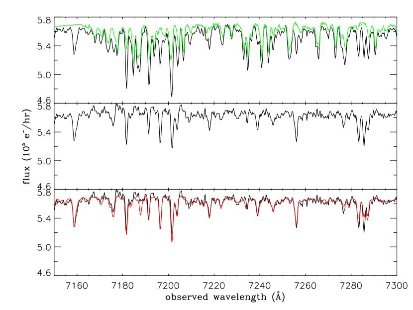
Figure 1.— A section of the spectrum for one star in M13. Top: The observed spectrum (black) with the telluric absorption template (green). Every feature in the telluric absorption template has a counterpart in the observed spectrum, but the reverse is not true. Middle: Applying the telluric absorption correction completely removes some of the absorption features seen in the raw spectrum, makes a few of the absorption features weaker, and leaves many of the features unaffected. Bottom: The telluric-divided spectrum (black, same as in middle panel) with the best-fit synthetic spectrum (red). The close agreement between the two spectra demonstrates that the features remaining in the observed spectrum are intrinsic to the star. Both the green and red lines have been scaled by the measured continuum.

Figure 1 demonstrates the efficacy of the telluric absorption removal. The upper panel shows part of an example spectrum before the telluric correction, along with the telluric absorption template. The middle panel shows the example spectrum after the correction. The bottom panel includes a synthetic stellar spectrum (see details in § 3), which shows that every absorption line left after the telluric correction is intrinsic to the star.

3.3. Radial velocities

We measure radial velocities of each target star to check its cluster membership and to shift its spectrum to the rest frame for abundance measurement. We cross-correlate each telluric-divided observed spectrum with a synthetic spectrum (see details in § 4) with $T_{\mathrm{eff}}=4500$ K, $\log g=1.5$, $\mathrm{[Fe/H]}=-1.5$, and $\mathrm{[\alpha/Fe]}=+0.2$ in the spectral region $8450~{}\mathrm{\AA}<\lambda<8700~{}\mathrm{\AA}$. This region includes the Ca II triplet, which is strong even in hot, extremely metal-poor stars, making it ideal for radial velocity determination in a wide range of stars. We shift the observed spectra to the rest frame to complete the remainder of the analysis.

3.4. Continuum determination

The abundance measurements are particularly sensitive to an accurate determination of the continuum. Underestimating the continuum will make absorption lines appear too shallow, and the derived abundances will be too low, the temperature too high, or both. The abundance analysis described in § 4 is insensitive to the global continuum shape and instead relies on high-frequency line-to-line variations in flux as a function of wavelength. Therefore, we have decided to focus on local continuum determination.

First, we determine the spectral regions free of stellar absorption. Following the procedures in § 4, we generate a synthetic spectrum between 6300 Å and 9100 Å of a star with $T_{\mathrm{eff}}=4300$ K, $\log g=1.5$, and $\mathrm{[Fe/H]}=-0.5$. The spectrum is smoothed through a moving Gaussian kernel of $\sigma=0.6$ Å to simulate the approximate spectral resolution of deimos. The synthetic spectrum has a perfectly flat continuum, and the units are such that the continuum is 1. We call spectral regions with synthetic flux greater than 0.96 and a minimum width of 0.5 Å “continuum regions.” Pixels at observed wavelengths outside of these regions will not contribute to the continuum determination of observed spectra.

Next, we compute the continuum. Each pixel in the continuum ($c_{j}$) is the weighted average of its neighboring pixels in the observed spectrum ($s_{i}$). The weight is a combination of the inverse variance ($\sigma_{i}^{2}$) and proximity in wavelength.

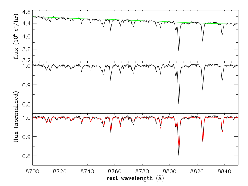
Figure 2.— A different section of the same star as in Fig. 1. Top: The observed spectrum (black) and the measured continuum (green). Middle: The observed spectrum divided by the continuum. Bottom: The continuum-normalized observed spectrum (black) with the best-fit synthetic spectrum (red), which has also been subjected to continuum normalization (see § 3.4 and § 4.4).

$$c_{j} = \frac{\sum_{i}s_{i}w_{i,j}m_{i}}{\sum_{i}w_{i,j}m_{i}}$$ (2)

$$w_{i,j} = \frac{1}{\sigma_{i}^{2}}\exp{\left(-\frac{(\lambda_{i}-\lambda_{j})^{2}}{2(10.0~{}\mathrm{\AA})^{2}}\right)}$$ (3)

$$m_{i} = \left\{\begin{array}[]{rl}1&\mathrm{if~{}}\lambda_{i}\in\mathrm{continuum~{}region}\\ 0&\mathrm{otherwise}\end{array}\right.$$ (6)

This process simultaneously accomplishes smoothing and interpolation across non-continuum regions. We normalize each observed spectrum by dividing by its measured continuum. Figure 2 shows the measured continuum in one example spectrum.

The continuum regions include some weak absorption lines, which will drag the continuum determination down by up to 4% in the coolest, most metal rich stars in our sample. In § 4.4, we determine the synthetic spectrum that most closely matches the observed spectrum. Before comparing a synthetic spectrum to the observed one, we apply the above continuum determination technique to both. Even though the synthetic spectrum has a perfectly flat continuum, application of this continuum determination technique causes the same degree of weak feature continuum suppression in both the synthetic and observed spectra, thereby correcting this effect.

3.5. Pixel mask

Table 2Spectral Masks

Feature	Lower Wavelength (Å)	Upper Wavelength (Å)
Telluric Absorption
B band	6864.000	7020.000
A band	7591.000	7703.000
strong telluric absorption	8225.000	8265.000
Stellar Absorption
Ca I $\lambda$6343	6341.000	6346.000
Ca I $\lambda$6362	6356.000	6365.000
H$\alpha$	6559.797	6565.797
K I $\lambda$7665	7662.000	7668.000
V I $\lambda$8116,$\lambda$8119 hyperfine structure	8113.000	8123.000
poorly modeled absorption in Arcturus (catalog NAME ARCTURUS)	8317.000	8330.000
Ca II $\lambda$8498	8488.023	8508.023
Ca II $\lambda$8542	8525.091	8561.091
Ca II $\lambda$8662	8645.141	8679.141
Mg I $\lambda$8807	8804.756	8809.756

Each spectrum has its own pixel mask. Table 2 lists spectral regions in observed and rest wavelength that may confuse the abundance analysis. The first part of the table lists regions of saturated or very strong telluric absorption. We mask the pixels that fall in these regions before we shift the spectrum to zero velocity. The second part of the table lists stellar absorption features that are difficult to model. We mask the pixels that fall in these regions after shifting the spectrum to zero velocity. These features include the strongest $\alpha$ element lines in the spectral range of deimos: the Ca II triplet and Mg I $\lambda$8807. The cores of the Ca II lines are formed very high in the stellar atmosphere out of local thermodynamic equilibrium (LTE). Because we could not synthetically reproduce the width and shape of the Mg I line in Arcturus (see § 4.2), we excluded it from the abundance analysis.

In addition to the standard mask in Table 2, we inspected each spectrum to mask improperly subtracted sky lines, cosmic rays, and other obvious instrumental artifacts.

4. Chemical Abundance Analysis

Table 3Grid of Synthetic Spectra

Parameter	Lower Limit	Upper Limit	Step	Number
$T_{\mathrm{eff}}$ (K)	4000	8000	$\left\{\begin{array}[]{rl}100&\mathrm{if~{}}T_{\mathrm{eff}}\leq 5500\\ 200&\mathrm{if~{}}T_{\mathrm{eff}}\geq 5600\end{array}\right.$	29
$\log g$	$\left\{\begin{array}[]{r}0.0\\ 0.0\\ 0.5\\ 0.5\\ 1.0\\ 0.5\\ 1.0\\ 1.0\\ 1.5\end{array}\right.$	$\begin{array}[]{rl}4.5&\mathrm{if~{}}T_{\mathrm{eff}}<4500\mathrm{~{}and~{}}\mathrm{[Fe/H]}<-2.5\\ 5.0&\mathrm{if~{}}(T_{\mathrm{eff}}<4500\mathrm{~{}and~{}}\mathrm{[Fe/H]}\geq-2.5)\mathrm{~{}or~{}}4500\leq T_{\mathrm{eff}}\leq 6000\\ 5.0&\mathrm{if~{}}6000<T_{\mathrm{eff}}\leq 7000\\ 5.0&\mathrm{if~{}}7000<T_{\mathrm{eff}}\leq 7200\mathrm{~{}and~{}}\mathrm{[Fe/H]}\geq-3.5\\ 5.0&\mathrm{if~{}}7000<T_{\mathrm{eff}}\leq 7200\mathrm{~{}and~{}}\mathrm{[Fe/H]}<-3.5\\ 5.0&\mathrm{if~{}}7200<T_{\mathrm{eff}}\leq 7500\mathrm{~{}and~{}}\mathrm{[Fe/H]}\geq-2.5\\ 5.0&\mathrm{if~{}}7200<T_{\mathrm{eff}}\leq 7500\mathrm{~{}and~{}}\mathrm{[Fe/H]}<-2.5\\ 5.0&\mathrm{if~{}}T_{\mathrm{eff}}>7500\mathrm{~{}and~{}}\mathrm{[Fe/H]}\geq-2.5\\ 5.0&\mathrm{if~{}}T_{\mathrm{eff}}>7500\mathrm{~{}and~{}}\mathrm{[Fe/H]}<-2.5\end{array}$	0.5	$\left\{\begin{array}[]{r}10\\ 11\\ 10\\ 10\\ 9\\ 10\\ 9\\ 9\\ 8\end{array}\right.$
[Fe/H]	$-4.0$	+0.0	0.1	41
[$\alpha$/Fe]	$-0.6$	$+1.0$	0.1	17
Total				210 902

The heart of this analysis is a very large grid of synthetic stellar spectra. The grid contains four dimensions: effective temperature ($T_{\mathrm{eff}}$), surface gravity ($\log g$), metallicity ([Fe/H]), and alpha enhancement ([$\alpha$/Fe]). Table 3 lists the details of the grid.

In this article, we use the standard spectroscopic abundance notation. The ratio of any two elements A and B in a star relative to their ratio in the Sun is

$$\mathrm{[A/B]}\equiv\log[n(\mathrm{A})/n(\mathrm{B})]-\log[n(\mathrm{A})/n(\mathrm{B})]_{\sun}$$ (7)

where $n$ is number density. [Fe/H] represents metallicity, the overall bulk content of the heavy elements. Because neutral Fe and neutral $\alpha$ element lines dominate the red spectra of stars in our $T_{\mathrm{eff}}$-$\log g$-[Fe/H] domain, we assume $\mathrm{[X/H]}=\mathrm{[Fe/H]}$ for most elements. We stress, however, that lines of all elements except the $\alpha$ elements contribute to the MRS measurement of [Fe/H]. The abundances of the $\alpha$ elements Mg, Si, S, Ar, Ca, and Ti are modified by the additional parameter [$\alpha$/Fe]:

$$\mathrm{[\alpha/H]}=\mathrm{[Fe/H]}+\mathrm{[\alpha/Fe]}\>.$$ (8)

The abundance enhancements of all six elements vary together.

We have found the best agreement with HRS by fixing the microturbulent velocity ($v_{t}$) to $\log g$ with an empirical relation. The best linear fit to the RGB sample ($\log g<3.3$) of Fulbright (2000) is

$$v_{t}=2.700-0.509\,\log g~{}\mathrm{km/s}.$$ (9)

4.1. Model atmospheres

The starting point for generating a synthetic spectrum is a model stellar atmosphere, which is a tabulation of temperature, pressure, electron fraction, and opacity as a function of optical depth. We choose to use the Castelli & Kurucz grid of models with no convective overshooting (Castelli et al., 1997). For atmospheres with $\mathrm{[Fe/H]}\geq-2.5$, we use the “ODFNEW” models, with updated opacity distribution functions (Castelli & Kurucz, 2004).

The published model atmosphere grid points of $T_{\mathrm{eff}}$, [Fe/H], and [$\alpha$/Fe] are coarser than the step sizes listed in Table 3. Therefore, for a fixed array of optical depths, we linearly interpolate temperatures, pressures, electron fractions, and opacities between model atmosphere grid points to generate a single model atmosphere for every grid point in Table 3.

The alpha enhancement changes the ionization balance and free election fraction in the atmosphere. ODFNEW ($\mathrm{[Fe/H]}\geq-2.5$) models are available for $\mathrm{[\alpha/Fe]}=0.0$ and $+0.4$. For synthesizing spectra with $\mathrm{[\alpha/Fe]}\leq 0.0$, we choose the former and for spectra with $\mathrm{[\alpha/Fe]}\geq+0.4$, we choose the latter. For intermediate values of $\mathrm{[\alpha/Fe]}$, we linearly interpolate between the two regimes. Atmospheres with $\mathrm{[Fe/H]}<-2.5$ are available only with $\mathrm{[\alpha/Fe]}=0.0$. For the model atmospheres only, the $\alpha$ elements are O, Ne, Mg, Si, S, Ar, Ca, and Ti.

4.2. Line lists

We assembled a line list of wavelengths, excitation potentials (EP), and oscillator strengths ($gf$) for atomic and molecular transitions that occur in the red spectral regions of stars in our stellar parameter range. In standard HRS analyses, it is often possible to use only transitions with accurately measured oscillator strengths. For this MRS analysis that covers a broad spectral range with many blended lines, we must use a database of lines with oscillator strengths of varying accuracy.

To begin, we queried the Vienna Atomic Line Database (VALD, Kupka et al., 1999) for all transitions of neutral or singly ionized atoms with $\mathrm{EP}<10$ eV and $\log gf>-5$. We supplemented the list with CN, $\mathrm{C}_{2}$, and MgH molecular transitions (Kurucz, 1992) and Li, Sc, V, Mn, Co, Cu, and Eu hyperfine transitions (Kurucz, 1993). By far, CN is the most important molecule for our red spectra. TiO is also strongly present in cool, metal-rich stars. However, the TiO system is extremely complex and difficult to model accurately. The large number of TiO electronic transitions in red spectra makes TiO spectral synthesis computationally daunting. Fortunately, TiO becomes a significant absorber only in metal-rich stars with $T_{\mathrm{eff}}<4000$ K. Therefore, we did not include TiO in our line list, and we chose $T_{\mathrm{eff}}=4000$ K as the grid’s lower limit.

Next, we generated synthetic spectra of the Sun and Arcturus (catalog NAME ARCTURUS) using our line list, model atmospheres as described in § 4.1, and the current version of the LTE spectral synthesis software MOOG (Sneden, 1973). The spectral range is 6300 Å to 9100 Å, and the resolution is 0.02 Å. The line broadening accounts for collisions with neutral hydrogen for for lines with tabulated damping constants (Barklem et al., 2000; Barklem & Aspelund-Johansson, 2005). For other lines, the Unsöld approximation multiplied by 6.3 gives the van der Waals line damping parameter, and MOOG calculates additional radiative and Stark broadening. However, the choice of damping parameter does not noticeably affect the spectra of low-pressure giant stars such as Arcturus, nor any star in the domain of $T_{\mathrm{eff}}$ and $\log g$ that we consider here.

The atmospheric parameters for the Sun are $T_{\mathrm{eff}}=5798$ K, $\log g=4.44$, and $\mathrm{[Fe/H]}=0.0$. For Arcturus (catalog NAME ARCTURUS), we adopt the atmospheric parameters and non-solar abundance ratios determined by Peterson et al. (1993): $T_{\mathrm{eff}}=4300$ K, $\log g=1.50$, and $\mathrm{[Fe/H]}=-0.50$. We compared these two synthetic spectra to the Hinkle et al. (2000) atlases of the Sun and Arcturus (catalog NAME ARCTURUS). After smoothing the synthetic spectra through a Gaussian kernel to match the line profiles of the atlas, we inspected the spectra in detail. First, we adjusted oscillator strengths of aberrant atomic lines in the solar synthetic spectrum until the strengths of the synthesized lines matched that of the observed lines. Then, we repeated the process for Arcturus (catalog NAME ARCTURUS), making adjustments that did not cause disagreement in the solar spectrum.

Table 4Line List

Wavelength (Å)	Species	EP (eV)	$\log gf$
8647.703	022.000	4.654	$-3.561$
8647.792	025.100	6.834	$-2.489$
8647.799	021.000	4.558	$-1.759$
8647.807	026.000	5.720	$-1.519$
8647.940	026.000	6.500	$-0.5$00
8648.024	021.000	4.126	$-2.710$
8648.040	607.000	1.093	$-3.058$
8648.366	607.000	1.093	$-1.096$
8648.400	607.000	0.912	$-2.763$
8648.455	014.000	6.210	+$0.0$00
8648.556	016.000	8.408	$-1.720$
8648.630	027.059	2.280	$-3.852$
8648.688	607.000	0.912	$-1.466$
8648.699	027.059	2.280	$-4.068$
8648.716	020.000	4.554	$-2.024$

Note. — Table 4 is published in its entirety in the electronic edition of the Astrophysical Journal. A portion is shown here for guidance regarding form and content. The first column is the line wavelength. The second is a code representing the atomic or molecular species. The integer part of the code is the element’s atomic number. Codes greater than 100 represent molecules. For example, 607 represents CN. The first decimal place of the code is the ionization state, where 0 is neutral. Remaining decimal places are mass numbers for isotopic hyperfine transitions. The third column is EP. The invented Fe I transitions have EP with fewer than three decimal places. The fourth column is oscillator strength. The transitions that we modified have oscillator strengths with fewer than three decimal places.

Occasionally, we encountered observed lines not present in the line list. Most of these cases could be resolved by relaxing the $\log gf>-5$ restriction. However, in cases where a single line was not represented in the VALD or Kurucz line lists, we invented a transition of Fe I of the EP and $gf$ required to reproduce the line’s observed strength in both the Sun and Arcturus (catalog NAME ARCTURUS). The final line list contains 30873 atomic and 17345 molecular transitions, representing 71 elements. Table 4 presents the entire line list.

With the final line list, the mean absolute deviation between the pixels of the solar spectrum and the pixels of its synthesis is $5.6\times 10^{-3}$, and the standard deviation is $1.3\times 10^{-2}$. For Arcturus (catalog NAME ARCTURUS), the mean absolute deviation is $9.4\times 10^{-3}$, and the standard deviation is $2.1\times 10^{-2}$. The units are such that the continuum is 1.

4.3. Synthetic spectra generation

We generate the library of synthetic spectra from the final line list. Each spectrum ranges from 6300 Å to 9100 Å with a resolution of 0.02 Å. To save computation time in the abundance determination, we bin each synthetic spectrum by a factor of 7 (0.14 Å resolution). When the binned and unbinned spectra are smoothed to the best resolution provided by deimos ($\sim 1.1$ Å FWHM), individual pixels in the binned spectra differ from the unbinned spectra by less than one part in $10^{3}$.

4.4. [Fe/H] and [$\alpha$/Fe] determination

Our continuum normalization for observed spectra (see § 3.4) may be depressed very slightly by weak absorption lines. To counteract this effect, we allow weak absorption in synthetic spectra to affect their normalizations in the same way that they affect observed spectra. First, we interpolate a synthetic spectrum onto the same wavelength array as the observed spectrum. Then, we smooth the synthetic spectrum through a Gaussian filter whose width is the observed spectrum’s measured spectral resolution as a function of wavelength (see § 2.2). To complete the renormalization, we divide the synthetic spectrum by the synthetic “continuum” determined exactly the same way as in § 3.4, including the continuum regions and weighting by the inverse variance of the observed spectrum.

We discard all stars with photometric $T_{\mathrm{eff}}<4000$ K because such stars are susceptible to TiO absorption, which we do not attempt to model. The coolest temperature on the synthetic grid is 4000 K for this reason.

Next, we compute $\chi^{2}$ for an initial guess at the four atmospheric parameters $T_{\mathrm{eff}}$, $\log g$, [Fe/H], and [$\alpha$/Fe]. A Levenberg-Marquardt optimization algorithm finds the values within the bounds of the grid that minimize $\chi^{2}$ computed from the difference between the observed spectrum and trial synthetic spectrum. We sample the parameter space between grid points by linearly interpolating the synthetic spectra at the neighboring grid points. The parameters for the best-fit spectrum are the final atmospheric parameters for the star. The fitting error on each parameter is $\sqrt{\sigma^{2}\chi^{2}}$ where $\sigma^{2}$ is the parameter’s diagonal element of the covariance matrix. The fitting errors are usually much smaller than the total error, including systematic error, which will be discussed in § 6. Fitting errors are particularly small for high S/N spectra.

Finding the global minimum $\chi^{2}$ in four dimensions is difficult. Surface gravity is particularly difficult to measure. First, the red spectral region contains very few gravity sensitive lines that are easy to model. Second, few transitions from ionized species are visible in our spectra, making surface gravity poorly constrained. To reduce the dimensionality of the parameter space, we fix $T_{\mathrm{eff}}$ and $\log g$ based on photometry (P. B. Stetson, private communication) and theoretical isochrones shifted to the distance modulus of the target. MRS abundances almost always agree with HRS abundances more closely when we fix $T_{\mathrm{eff}}$ and $\log g$ photometrically. Harris (1996, revised 2003) provides the distance modulus and reddening of each cluster.

For the GCs in this article, we use 14.0 Gyr, $\mathrm{[\alpha/Fe]}=+0.3$ isochrones from the Yonsei-Yale group (YY, Demarque et al., 2004). $T_{\mathrm{eff}}$ and $\log g$ are mostly insensitive to age and $\alpha$ enhancement. Given a star’s $I$ magnitude and $V-I$ color, we linearly interpolate between tracks of constant age to recover $T_{\mathrm{eff}}$ and $\log g$. (We do not have $I$ measurements for a few stars in M13 (catalog ) nor any star in NGC 7492 (catalog ). Instead, we use $V$ and $B-V$.) We have also experimented with Victoria-Regina (VandenBerg et al., 2006) and Padova (Girardi et al., 2002) isochrones. Although the Padova photometric [Fe/H] is quite different from the other two sets of isochrones near the tip of the RGB, the photometric $T_{\mathrm{eff}}$ and $\log g$ do not change enough to affect abundance analysis. We have also compared theoretical YY temperatures to the empirical temperatures of Ramírez & Meléndez (2005, RM05). For $T_{\mathrm{eff}}\lesssim 4800$ K, the average discrepancy $\Delta T_{\mathrm{eff}}<50$ K. For $T_{\mathrm{eff}}\gtrsim 5000$ K, the RM05 $T_{\mathrm{eff}}$ tends to be up to 250 K lower than the YY $T_{\mathrm{eff}}$. Given their success in reproducing GC abundances (§ 5.2), we have chosen to use YY temperatures.

Future applications of this method to inhomogeneous stellar populations may require an assumption of the age or iteration of the age until the spectroscopic [Fe/H] agrees with the photometric [Fe/H]. In theory, this iteration will give the age of the star. However, photometric errors and the systematic errors in both abundance measurement methods will undoubtedly make such an age very uncertain. In reality, $T_{\mathrm{eff}}$ and $\log g$ change little with age or metallicity for a given $V-I$ color, so the assumed isochrone parameters hardly affect the abundance results.

5. Results and comparison to HRS abundances

To demonstrate the effectiveness of the MRS abundance technique, we have observed GCs specifically to compare MRS to HRS metallicities and $\alpha$ enhancements. In this section, we present those comparisons and examine MRS results for systematic trends.

5.1. $T_{\mathrm{eff}}$

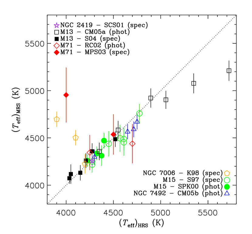
Figure 3.— $T_{\mathrm{eff}}$ determined from MRS without photometric information for individual stars (this work) vs. $T_{\mathrm{eff}}$ used in HRS studies of the same stars. $(T_{\mathrm{eff}})_{\mathrm{HRS}}$ is not necessarily determined spectroscopically. The figure legend indicates whether $(T_{\mathrm{eff}})_{\mathrm{HRS}}$ is determined spectroscopically (“spec”) or photometrically (“phot”). At $T_{\mathrm{eff}}>5000$ K, MRS analysis may underpredict $T_{\mathrm{eff}}$ because at high temperatures, lines with low EPs become immeasurably weak. Alternatively, the photometric temperatures for M13 based on theoretical atmospheres (Cohen & Meléndez, 2005a) may be overestimates. The dotted line is one-to-one. The following references provide $(T_{\mathrm{eff}})_{\mathrm{HRS}}$: SCS01: Shetrone et al. (2001), CM05a: Cohen & Meléndez (2005a), S04: Sneden et al. (2004), RC02: Ramírez & Cohen (2002), MPS03: Mishenina et al. (2003), K98: Kraft et al. (1998), S97: Sneden et al. (1997), SPK00: Sneden et al. (2000), and CM05b: Cohen & Meléndez (2005b).

The MRS technique can recover $T_{\mathrm{eff}}$ even without photometry. Figure 3 shows the $T_{\mathrm{eff}}$ of the best-fit atmospheric parameters when we allow $T_{\mathrm{eff}}$, $\log g$, [Fe/H], and [$\alpha$/Fe] to vary compared to the published $T_{\mathrm{eff}}$ used in HRS studies of the same stars. Not all authors of HRS studies determine $T_{\mathrm{eff}}$ spectroscopically. The figure legend indicates which HRS studies choose $T_{\mathrm{eff}}$ such that lines of different excitation potential yield the same abundance (“spec”) and which HRS studies rely exclusively on broadband photometry to determine $T_{\mathrm{eff}}$ (“phot”).

$(T_{\mathrm{eff}})_{\mathrm{MRS}}$ reproduces $(T_{\mathrm{eff}})_{\mathrm{HRS}}$ very well in most cases. The absolute deviation for 77% of stars falls within 150 K. At $T_{\mathrm{eff}}>5000$ K, MRS analysis underpredicts $T_{\mathrm{eff}}$ because at high temperatures, lines with low EPs become immeasurably weak. [An alternative explanation is that the photometric temperatures of Cohen & Meléndez (2005a) could be inaccurate.] Spectroscopic temperature is measured by comparing the strengths of lines with a range of EP. Without the low-EP lines, the temperature is difficult to measure. Fixing $T_{\mathrm{eff}}$ photometrically alleviates this problem and also eliminates the large random error in a spectroscopic $T_{\mathrm{eff}}$ of lower S/N stars. For the remainder of this article, both $T_{\mathrm{eff}}$ and $\log g$ are set by photometry.

5.2. [Fe/H]

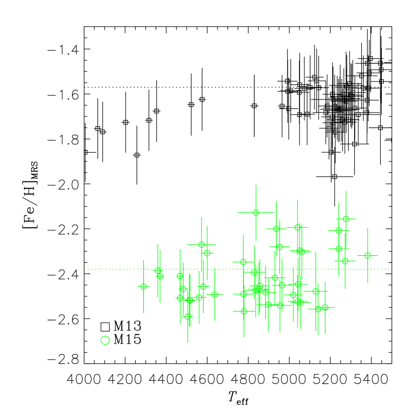
Figure 4.— $\mathrm{[Fe/H]}_{\mathrm{MRS}}$ vs. $T_{\mathrm{eff}}$ determined from $V-I$ color of individual stars in M13 and M15. (A few stars in M13 rely on $B-V$ rather than $V-I$.) The lack of a trend suggests little systematic covariance between measurements of $\mathrm{[Fe/H]}_{\mathrm{MRS}}$ and $T_{\mathrm{eff}}$. The dotted lines show $\mathrm{[Fe/H]}_{\mathrm{HRS}}$ (Pritzl et al., 2005).

We expect any spread in [Fe/H] within a single GC to be random error because these GCs are monometallic. Correlation of [Fe/H] with other parameters can indicate systematic errors. First, we show in Fig. 4 the spectroscopic [Fe/H] vs. photometric $T_{\mathrm{eff}}$ in M13 (catalog ) and M15 (catalog ). In all of M15 (catalog ) and above 5000 K in M13 (catalog ), we see only random scatter. The bright, cool stars near the tip of the RGB in M13 (catalog ) show a slight positive slope of $\sim 0.1$ dex from 4000 K to 5000 K. The covariance is undesirable but not unexpected. Both higher temperatures and lower metallicities weaken absorption lines. The magnitude and significance of the trend are small and restricted to the hottest stars. Furthermore, we emphasize that M13 (catalog ) is the worst case. No other GC shows this correlation.

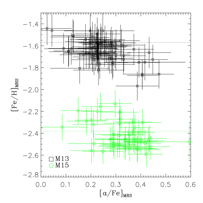
Figure 5.— $\mathrm{[Fe/H]}_{\mathrm{MRS}}$ vs. $\mathrm{[\alpha/Fe]}_{\mathrm{MRS}}$ of individual stars in M13 and M15. The lack of a trend suggests little systematic covariance between measurements of $\mathrm{[\alpha/Fe]}_{\mathrm{MRS}}$ vs. $\mathrm{[Fe/H]}_{\mathrm{MRS}}$. The dotted lines show $\mathrm{[Fe/H]}_{\mathrm{HRS}}$ (Pritzl et al., 2005).

We also expect no correlation between [$\alpha$/Fe] and [Fe/H] within a single GC. Both [$\alpha$/Fe] and [Fe/H] affect the strength of $\alpha$ element absorption lines. If there were a systematic trend, we would expect the two parameters to be anti-correlated. No cluster shows a convincing anti-correlation. Figure 5 shows both parameters for M13 (catalog ) and M15 (catalog ). M13 (catalog ) is again the worst case, and the significance of any trend is destroyed by removing the one or two points with the most discrepant [Fe/H].

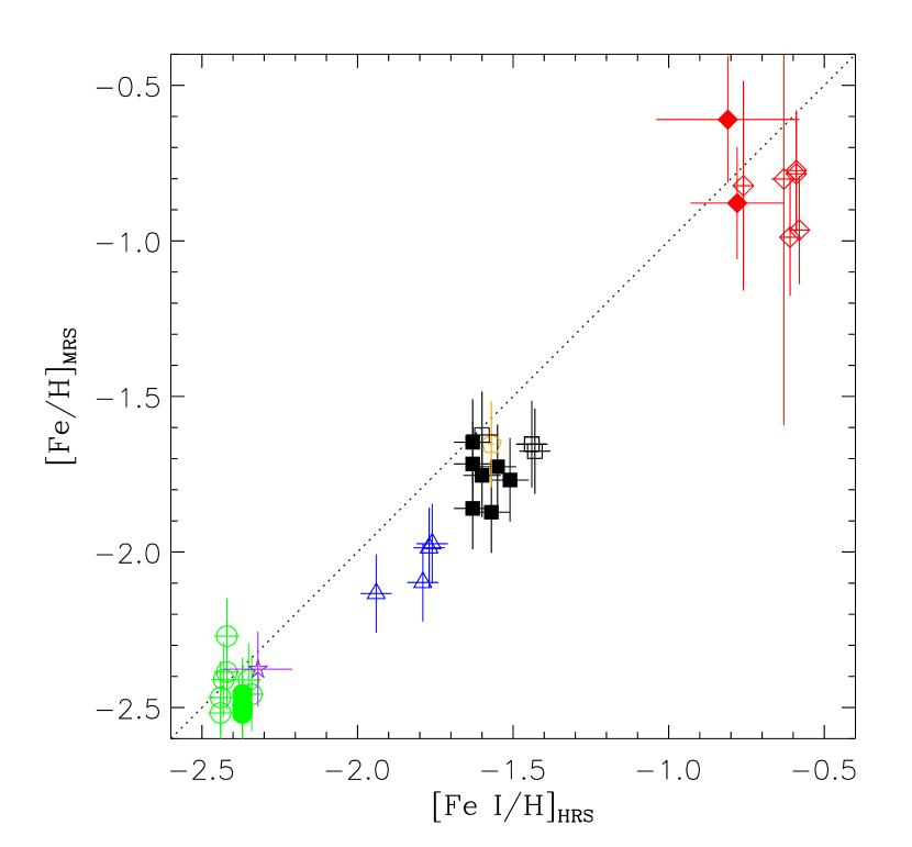
Figure 6.— This work’s [Fe/H] vs. [Fe I/H] determined from neutral iron lines in HRS. The dotted line is one-to-one. The symbols, colors, and references are the same as in Fig. 3.

The MRS technique matches the metallicities determined from HRS to within the HRS metallicity scatter for a given GC. Figure 6 shows [Fe/H] of the best-fit atmospheric parameters (where photometry determines $T_{\mathrm{eff}}$ and $\log g$) compared to $\mathrm{[Fe/H]}_{\mathrm{HRS}}$ determined from Fe I lines in the range $-2.38<\mathrm{[Fe/H]}<-0.76$. We choose Fe I because Fe I lines greatly outnumber Fe II lines in the deimos spectra with our range of $T_{\mathrm{eff}}$ and $\log g$. Although these GCs are almost certainly monometallic, we have plotted the measurements for individual stars on both axes. The range of $\mathrm{[Fe/H]}_{\mathrm{HRS}}$ within a single GC, particularly depending on the authors of the measurement, demonstrates the uncertainty to which the mean metallicity is known. The MRS measurements do not fall outside of this scatter.

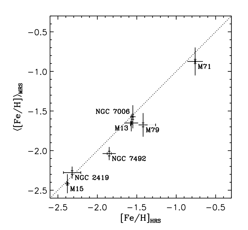
Figure 7.— Mean [Fe/H] values in GCs observed with deimos vs. values of [Fe/H] determined from HRS (Pritzl et al., 2005). The dotted line is one-to-one. The full error bars are weighted sample standard deviations, and the hash marks along the error bars are weighted errors on the mean. The HRS errors are weighted by the inverse square of the measurement errors of all of the individual stars in the following references. M79: Gratton & Ortolani (1989), NGC 2419 (the HRS error bar is the individual measurement error for the only star available): Shetrone et al. (2001), M13: Sneden et al. (2004) and Cohen & Meléndez (2005a), M71: Gratton et al. (1986), Sneden et al. (1994), Ramírez & Cohen (2002), and Mishenina et al. (2003), NGC 7006: Kraft et al. (1998), M15: Sneden et al. (1997) and Sneden et al. (2000), NGC 7492: Cohen & Meléndez (2005b)

Table 5Average Globular Cluster Abundances Comparison

Cluster	$N_{\mathrm{HRS}}$	$\mathrm{[Fe/H]}_{\mathrm{PVI05}}$	$\langle\mathrm{[\alpha/Fe]}_{\mathrm{HRS}}\rangle$	$N_{\mathrm{DEIMOS}}$	$\langle\mathrm{[Fe/H]}_{\mathrm{MRS}}\rangle$	$\mathrm{rms}\,(\mathrm{[Fe/H]}_{\mathrm{MRS}})$	$\langle\mathrm{[\alpha/Fe]}_{\mathrm{MRS}}\rangle$	$\mathrm{rms}\,(\mathrm{[\alpha/Fe]}_{\mathrm{MRS}})$
M79 (catalog )	02	$-1.42$	$+0.26\pm 0.08$	33	$-1.69\pm 0.02$	0.15	$+0.27\pm 0.01$	0.11
NGC 2419 (catalog )	01	$-2.32$	$+0.20\pm 0.08$	30	$-2.28\pm 0.02$	0.08	$+0.28\pm 0.01$	0.09
M13 (catalog )	60	$-1.57$	$+0.20\pm 0.01$	69	$-1.66\pm 0.02$	0.11	$+0.25\pm 0.01$	0.09
M71 (catalog )	40	$-0.76$	$+0.27\pm 0.01$	47	$-0.92\pm 0.04$	0.17	$+0.27\pm 0.01$	0.17
NGC 7006 (catalog )	06	$-1.55$	$+0.24\pm 0.01$	20	$-1.59\pm 0.03$	0.13	$+0.35\pm 0.01$	0.08
M15 (catalog )	49	$-2.38$	$+0.42\pm 0.03$	44	$-2.42\pm 0.01$	0.12	$+0.33\pm 0.01$	0.07
NGC 7492 (catalog )	04	$-1.85$	$+0.23\pm 0.02$	21	$-2.04\pm 0.02$	0.08	$+0.32\pm 0.02$	0.10

Note. — The rms values and errors on the mean are weighted by the inverse square of individual measurement errors.

We measure individual metallicities for all stars that we observe. We eliminate non-members by radial velocity, and we discard stars with photometric $T_{\mathrm{eff}}$ outside the range of the spectral grid. We also discard HB stars and stars with noticeable TiO absorption. Figure 7 shows the weighted mean of $\mathrm{[Fe/H]}_{\mathrm{MRS}}$ of all the stars in each cluster. The abscissa is $\mathrm{[Fe/H]}_{\mathrm{HRS}}$ from the compilation of Pritzl et al. (2005). Two types of errors bars are shown on both axes: the standard error on the mean and the sample standard deviation. The latter represents the typical measurement error on one star. The HRS error bars are determined from $\mathrm{[Fe/H]}_{\mathrm{HRS}}$ of individual stars in the references given in the figure caption. The error bars for both MRS and HRS are weighted by the inverse square of the individual measurement errors. Table 5 lists the same data along with the number of stars in each sample. The HRS measurements for NGC 2419 (catalog ), M79 (catalog ), and NGC 7492 (catalog ) are based respectively on only 1, 2, and 4 stars. We suggest that, in these cases, a cluster’s mean [Fe/H] may be more precisely determined with our larger MRS samples.

Table 7 lists MRS results for individual stars. Where available, all three photometric magnitudes ($B$, $V$, and $I$) are given, but only two determine $T_{\mathrm{eff}}$ and $\log g$. $V$ and $I$ are preferred. $T_{\mathrm{eff}}$ and $\log g$ in this table are the values that we have determined photometrically. The last three columns are data from and references to HRS studies for the stars in common between the MRS and HRS datasets.

All GCs seem to display internal variations in [C/H] and [N/H] (e.g., Grundahl, 1999). Cohen et al. (2005) show ranges of 2–3 dex of [N/H] in five GCs, including M13 (catalog ), M71 (catalog ), and M15 (catalog ). The variations could alter the strength of CN absorption. M71 (catalog ) is the only GC in our sample metal-rich enough to exhibit strong red CN absorption. If star-to-star CN abundance variations affect $\mathrm{[Fe/H]}_{\mathrm{MRS}}$, then the metallicity determined only from the spectral region affected by CN (7850–8400 Å) should differ from the metallicity determined from the rest of the spectrum. We subjected M71 (catalog ) to this test, and [Fe/H] measurements from the two cases agree very closely for every star. CN abundance variations, if they exist, do not appear to contribute to the error on individual stars or to the large scatter in $\mathrm{[Fe/H]}_{\mathrm{MRS}}$ for M71 (catalog ).

5.3. [$\alpha$/Fe]

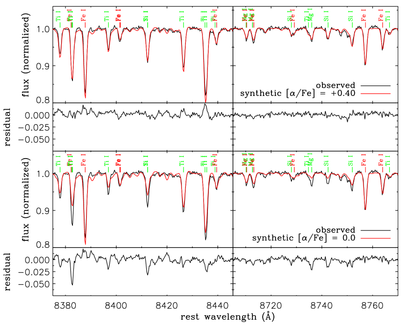
Figure 8.— Top: Portions of an observed spectrum of a star in M13 (black) and the best fit synthetic spectrum (red), which has $\mathrm{[\alpha/Fe]}=+0.40$. Fe lines are labeled in red and $\alpha$ element lines are labeled in green. The residual is the difference between the observed and synthetic spectra. Bottom: The same observed spectrum (black) and a synthetic spectrum (red) with the same parameters as the synthetic spectrum in the top panel except that $\mathrm{[\alpha/Fe]}=0.0$. The observed spectrum is highly inconsistent with the solar value of [$\alpha$/Fe].

MRS can give an abundance dimension beyond metallicity. Most of the stellar absorption lines visible in deimos spectra are from Fe I, but there are a comparable number of $\alpha$ element absorption lines. By far, the most abundant are Ti, Si, Ca, and Mg, in order of decreasing prevalence. Figure 8 shows two spectral regions with high concentrations of lines from all of these elements except Ca. The figure also shows two synthetic spectra that are identical except for their values of [$\alpha$/Fe]. The observed spectrum is consistent with the synthetic spectrum for which $\mathrm{[\alpha/Fe]}=+0.40$, but highly inconsistent with the synthetic spectrum for which $\mathrm{[\alpha/Fe]}=0.0$. The discrepancy demonstrates that MRS can easily distinguish between the halo plateau and solar values of [$\alpha$/Fe].

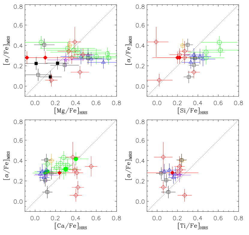
Figure 9.— $\mathrm{[\alpha/Fe]}_{\mathrm{MRS}}$ vs. individual $\alpha$ element abundances determined from HRS. The dotted lines are one-to-one. The symbols, colors, and references are the same as in Fig. 3.

In order to build additional confidence in the ability of MRS to determine [$\alpha$/Fe], we compare values of $\mathrm{[\alpha/Fe]}_{\mathrm{MRS}}$ to HRS measurements. Figure 9 shows $\mathrm{[\alpha/Fe]}_{\mathrm{MRS}}$ compared to HRS measurements of [Mg/Fe], [Si/Fe], [Ca/Fe], and [Ti/Fe]. All four plots show weak or no correlations. The lackluster agreement is not surprising because $\mathrm{[\alpha/Fe]}_{\mathrm{MRS}}$ is a weighted combination of all four elements.

To better compare MRS and HRS results, we define $\mathrm{[\alpha/Fe]}_{\mathrm{HRS}}$, which is a weighted mean of the four $\alpha$ element ratios.

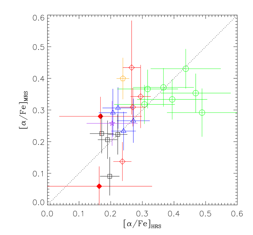
Figure 10.— $\mathrm{[\alpha/Fe]}_{\mathrm{MRS}}$ vs. a weighted average of the available [Mg/Fe], [Si/Fe], [Ca/Fe], and [Ti/Fe] HRS measurements for individual stars. Eqs. 5.3 and 5.3 give the formulas for deriving $\mathrm{[\alpha/Fe]}_{\mathrm{HRS}}$ and its error from the individual element measurements. The dotted line is one-to-one. The symbols, colors, and references are the same as in Fig. 3. See § 5.3 for a discussion of the large values of $\mathrm{[\alpha/Fe]}_{\mathrm{HRS}}$ for M15 (green points).

$$\mathrm{[\alpha/Fe]}_{\mathrm{HRS}} = (\gamma_{\mathrm{Mg}}\,\mathrm{[Mg/Fe]}+4\gamma_{\mathrm{Si}}\,\mathrm{[Si/Fe]}$$

$$+2\gamma_{\mathrm{Ca}}\,\mathrm{[Ca/Fe]}+6\gamma_{\mathrm{Ti}}\,\mathrm{[Ti/Fe]})$$

$$\times(\gamma_{\mathrm{Mg}}+4\gamma_{\mathrm{Si}}+2\gamma_{\mathrm{Ca}}+6\gamma_{\mathrm{Ti}})^{-1}$$

$$\delta\mathrm{[\alpha/Fe]}_{\mathrm{HRS}} = \big{[}\gamma_{\mathrm{Mg}}\left(\delta\mathrm{[Mg/Fe]}\right)^{2}+\gamma_{\mathrm{Si}}\left(4\,\delta\mathrm{[Si/Fe]}\right)^{2}$$

$$+\gamma_{\mathrm{Ca}}\left(2\,\delta\mathrm{[Ca/Fe]}\right)^{2}+\gamma_{\mathrm{Ti}}\left(6\,\delta\mathrm{[Ti/Fe]}\right)^{2}\big{]}^{1/2}$$

$$\times(\gamma_{\mathrm{Mg}}+4\gamma_{\mathrm{Si}}+2\gamma_{\mathrm{Ca}}+6\gamma_{\mathrm{Ti}})^{-1}$$

The $\gamma_{\mathrm{X}}$ coefficients are 1 if the element X has a published HRS value and 0 otherwise. $\delta\mathrm{[X/Fe]}$ is the published error. For those studies that quote [X/H] instead of [X/Fe], $\delta\mathrm{[X/Fe]}=\sqrt{(\delta\mathrm{[X/H]})^{2}+(\delta\mathrm{[Fe/H]})^{2}}$. The weights 1, 4, 2, and 6 mimic the relative presence of absorption from the four elements. This combination of weights also gives good correlation between $\mathrm{[\alpha/Fe]}_{\mathrm{MRS}}$ and $\mathrm{[\alpha/Fe]}_{\mathrm{HRS}}$, shown in Fig. 10. These data are also listed in Table 7. Although the weights in $\mathrm{[\alpha/Fe]}_{\mathrm{HRS}}$ approximate the weights that the individual elements receive in determining $\mathrm{[\alpha/Fe]}_{\mathrm{MRS}}$, matching the elemental averages exactly is not possible. Therefore, the comparisons between $\mathrm{[\alpha/Fe]}_{\mathrm{MRS}}$ and $\mathrm{[\alpha/Fe]}_{\mathrm{HRS}}$ are approximate checks of agreement.

Three studies deserve particular mention. The M15 (catalog ) measurements of Sneden et al. (2000) use Hydra spectra, which have lower spectral resolution than most HRS studies. They do not attempt to measure Mg, and most of their stars do not display enough Si or Ti absorption to permit accurate measurements of those elemental abundances. Furthermore, their Ca measurements are based on only one line. The M13 (catalog ) measurements of Sneden et al. (2004) do not include Si, Ca, or Ti. They do measure Mg, but Mg is the least visible $\alpha$ element in the deimos spectra. For these reasons, we exclude the $\mathrm{[\alpha/Fe]}_{\mathrm{HRS}}$ measurements of Sneden et al. (2000) and Sneden et al. (2004) from Fig. 10 and Table 7. We also draw attention to the M15 (catalog ) measurements of Sneden et al. (1997). They measure particularly large values for [Si/Fe], and they do not recover [Ti/Fe] for any of the stars that are in common between their HRS sample and our MRS sample. Therefore, $\mathrm{[\alpha/Fe]}_{\mathrm{HRS}}$ has a different meaning for the M15 (catalog ) data (green points in Fig. 10) than for the data from other clusters.

Figure 11.— Mean cluster values of $\mathrm{[\alpha/Fe]}_{\mathrm{MRS}}$ vs. $\mathrm{[\alpha/Fe]}_{\mathrm{HRS}}$. The range of [$\alpha$/Fe] in these GCs is very small, but the points are roughly consistent with the one-to-one line (dotted line). See § 5.3 for a discussion of the large value of $\langle\mathrm{[\alpha/Fe]}_{\mathrm{HRS}}\rangle$ for M15.

Comparing individual stars limits the sample to stars observed with both MRS and HRS. In order to draw on the full set of stars observed with either MRS or HRS, we compute mean values of [$\alpha$/Fe] for entire clusters. $\langle\mathrm{[\alpha/Fe]}\rangle$ is weighted by the inverse square of $\delta\mathrm{[\alpha/Fe]}$. Figure 11 shows the comparison. These averages are also listed in Table 5. The range of $\langle\mathrm{[\alpha/Fe]}\rangle$ for these GCs is very small, but $\langle\mathrm{[\alpha/Fe]}\rangle_{\mathrm{MRS}}$ and $\langle\mathrm{[\alpha/Fe]}\rangle_{\mathrm{HRS}}$ agree to $\lesssim 0.1$ dex for all clusters.

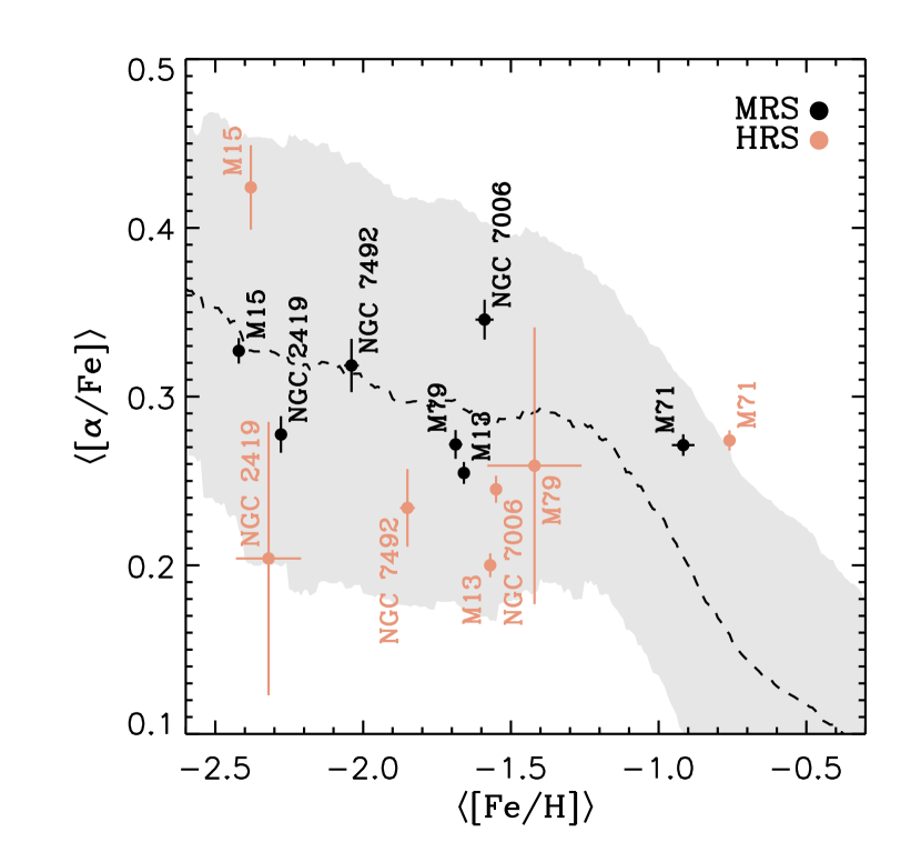
Figure 12.— Mean cluster values of [$\alpha$/Fe] vs. [Fe/H] for MRS (black) and HRS (pink). For comparison, we show the relation for MW stars from Venn et al. (2004). The dashed line is the average [$\alpha$/Fe] in a moving window with a half width of 0.5 dex in [Fe/H], and the shaded region is the rms spread. $\mathrm{[\alpha/Fe]}_{\mathrm{MRS}}$ is very near the MW halo plateau value of $\mathrm{[\alpha/Fe]}=+0.3$ for every cluster.

Finally, we show $\langle\mathrm{[\alpha/Fe]}\rangle$ vs. $\langle\mathrm{[Fe/H]}\rangle$ in Fig. 12. Also shown is the relationship between these two quantities for MW stars tabulated by Venn et al. (2004). The $\langle\mathrm{[Fe/H]}\rangle$ values from both MRS and HRS are consistent with the halo plateau value of $\mathrm{[\alpha/Fe]}\sim+0.3$.

6. Quantification of Abundance Errors

6.1. Total Error on [Fe/H]

The Levenberg-Marquardt algorithm which determines the best-fit synthetic spectrum by minimizing $\chi^{2}$ gives an estimate of the fitting error based on the depth of the $\chi^{2}$ minimum in parameter space. However, the fitting error is usually a small part of the total error. The major sources of error in high S/N spectra are errors in atmospheric parameters and imperfect spectral modeling. Two effects make the total error a function of [Fe/H]. First, higher metallicity spectra are more sensitive to errors in $T_{\mathrm{eff}}$ and $\log g$ (see § 6.3). Second, higher metallicity spectra exhibit more complex absorption from molecular transitions not seen at lower metallicity.

In order to quantify the total error on $\mathrm{[Fe/H]}_{\mathrm{MRS}}$, for each cluster we find the systematic error $\delta_{\mathrm{sys}}\mathrm{[Fe/H]}_{\mathrm{MRS}}$ that satisfies

Figure 13.— The systematic error in [Fe/H] as a function of the mean [Fe/H] for each cluster. The line is the best fit of the function $\ln\left(e^{0.1}+e^{a+bx}\right)$.

$$\mathrm{rms}\,\left(\frac{\mathrm{[Fe/H]}_{\mathrm{MRS}}-\langle\mathrm{[Fe/H]}_{\mathrm{MRS}}\rangle}{\sqrt{\left(\delta_{\mathrm{fit}}\mathrm{[Fe/H]}_{\mathrm{MRS}}\right)^{2}+\left(\delta_{\mathrm{sys}}\mathrm{[Fe/H]}_{\mathrm{MRS}}\right)^{2}}}\right)=1\>.$$ (12)

Figure 13 shows the results. $\delta_{\mathrm{sys}}\mathrm{[Fe/H]}_{\mathrm{MRS}}$ appears to approach 0.1 at low [Fe/H] and increase as [Fe/H] rises above $-1.6$. We choose to fit a function that asymptotically approaches a constant at low [Fe/H] and increases linearly at large [Fe/H]. A function that satisfies these requirements is $\ln\left(e^{0.1}+e^{a+bx}\right)$. The least-squares fit with uniform weighting is

$$\delta_{\mathrm{sys}}\mathrm{[Fe/H]}_{\mathrm{MRS}}=\ln\left(e^{0.1}+e^{-0.758+1.86\,\mathrm{[Fe/H]}}\right)\>.$$ (13)

The total error is

$$\delta_{\mathrm{tot}}\mathrm{[Fe/H]}_{\mathrm{MRS}}=\sqrt{\left(\delta_{\mathrm{fit}}\mathrm{[Fe/H]}_{\mathrm{MRS}}\right)^{2}+\left(\delta_{\mathrm{sys}}\mathrm{[Fe/H]}_{\mathrm{MRS}}\right)^{2}}\>.$$ (14)

The error bars on $\mathrm{[Fe/H]}_{\mathrm{MRS}}$ for all plots and tables in this article are calculated from Eqs. 13 and 14.

6.2. Total Error on [$\alpha$/Fe]

We repeat the same procedure to find the systematic error in $\mathrm{[\alpha/Fe]}_{\mathrm{MRS}}$. However, we compute the deviation from the $\mathrm{[\alpha/Fe]}_{\mathrm{HRS}}$—accounting for HRS error—rather than the mean of $\mathrm{[\alpha/Fe]}_{\mathrm{MRS}}$.

$$\mathrm{rms}\,\left(\frac{\mathrm{[\alpha/Fe]}_{\mathrm{MRS}}-\mathrm{[\alpha/Fe]}_{\mathrm{HRS}}}{\sqrt{\left(\delta_{\mathrm{fit}}\mathrm{[\alpha/Fe]}_{\mathrm{MRS}}\right)^{2}+\left(\delta_{\mathrm{sys}}\mathrm{[\alpha/Fe]}_{\mathrm{MRS}}\right)^{2}+\left(\delta\mathrm{[\alpha/Fe]}_{\mathrm{HRS}}\right)^{2}}}\right)=1$$ (15)

The value that satisfies this equation is $\delta_{\mathrm{sys}}\mathrm{[\alpha/Fe]}_{\mathrm{MRS}}=0.03$. The total error is

$$\delta_{\mathrm{tot}}\mathrm{[\alpha/Fe]}_{\mathrm{MRS}}=\sqrt{\left(\delta_{\mathrm{fit}}\mathrm{[\alpha/Fe]}_{\mathrm{MRS}}\right)^{2}+\left(\delta_{\mathrm{sys}}\mathrm{[\alpha/Fe]}_{\mathrm{MRS}}\right)^{2}}\>.$$ (16)

The error bars on $\mathrm{[\alpha/Fe]}_{\mathrm{MRS}}$ for all plots and tables in this article are calculated from Eq. 16.

6.3. Errors from Atmospheric Parameters

Errors in $T_{\mathrm{eff}}$ and $\log g$ have the potential to change the measured abundances significantly. The total $\mathrm{[Fe/H]}_{\mathrm{MRS}}$ error estimates in § 6.1 account for random error about the true values of $T_{\mathrm{eff}}$ and $\log g$, but not systematic offsets. The total $\mathrm{[\alpha/Fe]}_{\mathrm{MRS}}$ error estimates in § 6.2 do account for both random and systematic error in the atmospheric parameters to the extend that $T_{\mathrm{eff}}$ and $\log g$ in the comparison HRS studies are accurate.

Table 6Errors from Atmospheric Parameters

Atmospheric Error	$\delta\mathrm{[Fe/H]}$	$\delta\mathrm{[\alpha/Fe]}$
$T_{\mathrm{eff}}-250~{}\mathrm{K}$	$-0.21\pm 0.08$	$+0.01\pm 0.12$
$T_{\mathrm{eff}}-125~{}\mathrm{K}$	$-0.10\pm 0.04$	$+0.01\pm 0.08$
$T_{\mathrm{eff}}+125~{}\mathrm{K}$	$+0.11\pm 0.05$	$-0.03\pm 0.06$
$T_{\mathrm{eff}}+250~{}\mathrm{K}$	$+0.20\pm 0.08$	$-0.07\pm 0.10$
$\log g-0.6$	$-0.06\pm 0.06$	$+0.00\pm 0.07$
$\log g-0.3$	$-0.03\pm 0.04$	$+0.01\pm 0.06$
$\log g+0.3$	$+0.04\pm 0.03$	$-0.01\pm 0.05$
$\log g+0.6$	$+0.07\pm 0.07$	$-0.01\pm 0.07$

We quantify the abundance error introduced by errors in atmospheric parameters by varying $T_{\mathrm{eff}}$ and $\log g$ for all stars in the GC sample. We recompute abundances at $T_{\mathrm{eff}}\pm 125~{}\mathrm{K}$, $T_{\mathrm{eff}}\pm 250~{}\mathrm{K}$, $\log g\pm 0.3$, and $\log g\pm 0.6$. Table 6 shows the differences in [Fe/H] and [$\alpha$/Fe] between the altered and unaltered atmospheres. The numbers presented are the mean difference and standard deviations for all stars in all seven GCs.

As expected, increasing $T_{\mathrm{eff}}$ causes [Fe/H] to increase because the synthetic atmosphere must have a higher density of absorbers to compensate for the temperature-induced weakening in line strength. Increasing $\log g$ also causes [Fe/H] to increase because a higher electron pressure increases the density of $\mathrm{H}^{-}$ ions. $\mathrm{H}^{-}$ is the dominant source of continuous optical and near-infrared opacity in these cool giants. Therefore, as $\log g$ increases, the decreasing ratio of line opacity to continuous opacity depresses line strength. The synthetic atmosphere needs to be more metal-rich to compensate. We also point out a few trends with $T_{\mathrm{eff}}$, $\log g$, and [Fe/H]:

1. $\delta\mathrm{[Fe/H]}_{\mathrm{MRS}}$ is gradually less sensitive to $\delta T_{\mathrm{eff}}$ as $T_{\mathrm{eff}}$ increases.

2. $\delta\mathrm{[Fe/H]}_{\mathrm{MRS}}$ does not show a trend with $\delta\log g$ as $\log g$ increases.

3. $\delta\mathrm{[Fe/H]}_{\mathrm{MRS}}$ does not show a trend with $\delta T_{\mathrm{eff}}$ as [Fe/H] increases.

4. $\delta\mathrm{[Fe/H]}_{\mathrm{MRS}}$ is gradually more sensitive to $\delta\log g$ as [Fe/H] increases.

5. On average, $\delta\mathrm{[\alpha/Fe]}_{\mathrm{MRS}}$ has the same sign as $\delta T_{\mathrm{eff}}$ for $T_{\mathrm{eff}}<4600~{}\mathrm{K}$ and the opposite sign otherwise. $\delta\mathrm{[\alpha/Fe]}_{\mathrm{MRS}}$ is most sensitive to $\delta T_{\mathrm{eff}}$ at low $T_{\mathrm{eff}}$.

6. $\delta\mathrm{[\alpha/Fe]}_{\mathrm{MRS}}$ does not show a trend with $\delta\log g$ as $\log g$ increases.

7. $\delta\mathrm{[\alpha/Fe]}_{\mathrm{MRS}}$ does not show any trends with [Fe/H].

6.4. Effect of Noise

Stars at the tip of the RGB in MW GCs are easy targets for high resolution spectrometers. The intended targets of the MRS method are much fainter. Therefore, we explore the effect of noise on the measurement of [Fe/H] and [$\alpha$/Fe]. To estimate S/N, we compute the absolute deviation from 1.0 of all pixels in the continuum regions (see § 3.4). We clip pixels that exceed 3 times this mean deviation. The S/N per pixel is the inverse of the mean absolute deviation of the remaining pixels. To convert to S/N per Å, multiply by 1.74, the inverse square root of the pixel scale.

Figure 14.— Examples of the Ca II triplet region of spectra at three different signal-to-noise ratios. These are three different stars in NGC 2419, obtained with 20 minutes of exposure time on deimos. Shown in each panel is the S/N, $I$ magnitude, and measured [Fe/H]. The value from one star (not shown) observed with HRS is $\mathrm{[Fe/H]}_{\mathrm{HRS}}=-2.32$ (Shetrone et al., 2001).

Figure 14 shows the Ca II triplet region of three deimos spectra of stars in NGC 2419 (catalog ) in three different S/N regimes. The three strongest lines are the Ca II triplet, and the five weaker lines are individual or blended Fe I transitions. We show the Ca II triplet to demonstrate spectral quality, but we do not use any spectral information from any of the three lines because we do not model them accurately. Instead, we use the weaker metal lines, any one of which is difficult to identify in low S/N spectra. As an ensemble over $\sim 2800$ Å of spectral range, they provide accurate abundances. Below, we discuss spectra at $\mathrm{S/N}\sim 10~{}\mathrm{\AA}^{-1}$, in which even the Ca II triplet is barely identifiable.

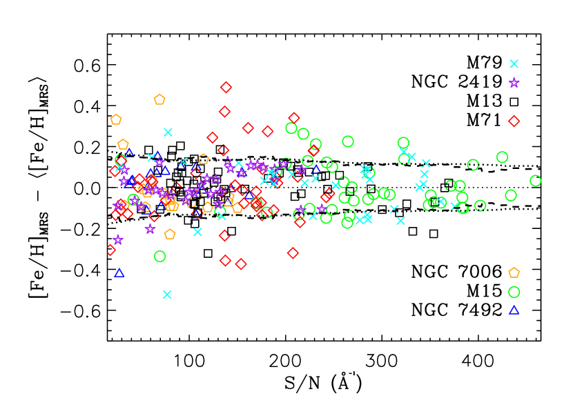
Figure 15.— The difference between individual measurements of $\mathrm{[Fe/H]}_{\mathrm{MRS}}$ and the cluster’s mean $\langle\mathrm{[Fe/H]}_{\mathrm{MRS}}\rangle$ vs. signal-to-noise ratio. The dashed line is the rms in a moving window with a half width of $50~{}\mathrm{\AA}^{-1}$. The dotted line is the average error determined from Eqs. 13 and 14 in the same moving window.

Figure 15 shows the difference between $\mathrm{[Fe/H]}_{\mathrm{MRS}}$ for an individual star and the mean $\mathrm{[Fe/H]}_{\mathrm{MRS}}$ that we measure for its cluster ($\Delta\mathrm{[Fe/H]}_{\mathrm{MRS}}$) vs. S/N. We also include the rms of all points in a moving window with a half width of $50~{}\mathrm{\AA}^{-1}$. At $\mathrm{S/N}>200~{}\mathrm{\AA}^{-1}$, the rms scatter in $\Delta\mathrm{[Fe/H]}$ is about 0.15 dex. The rms rises to about 0.20 dex in the range $20~{}\mathrm{\AA}^{-1}<\mathrm{S/N}<200~{}\mathrm{\AA}^{-1}$. Errors such as these are about the magnitude of typical HRS abundance errors. We also include the average $\delta_{\mathrm{tot}}\mathrm{[Fe/H]}_{\mathrm{MRS}}$ in the same moving window. The close agreement between the two error averages demonstrates that we determine $\delta_{\mathrm{tot}}\mathrm{[Fe/H]}_{\mathrm{MRS}}$ well.

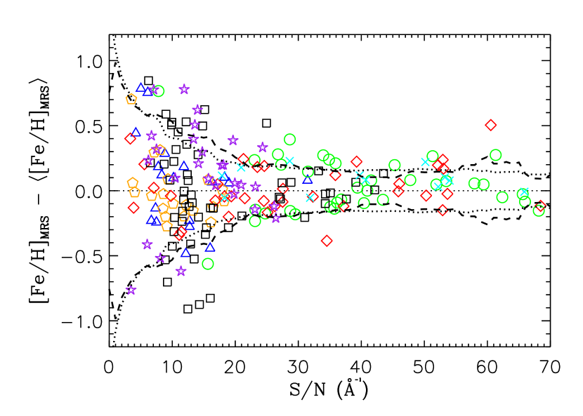
Figure 16.— Same as Fig. 15 for measurements injected with artificial noise. The ranges of both axes are different from Fig. 15. The dashed line is the rms in a moving window with a half width of $5~{}\mathrm{\AA}^{-1}$. The dotted line is the average error determined from Eqs. 13 and 14 in the same moving window.

In order to better scrutinize noisier spectra at $\mathrm{S/N}<20~{}\mathrm{\AA}^{-1}$, we inject the raw spectra with Gaussian random noise proportional to the square root of the measured variance in each pixel. On average, the S/N of a given spectrum decreases by a factor of 10. We repeat the complete analysis, including continuum determination and velocity cross-correlation. Figure 16 shows that rms scatter gradually increases as S/N decreases, but even at $\mathrm{S/N}\sim 10~{}\mathrm{\AA}^{-1}$, the rms scatter is only 0.5 dex. The Ca II triplet is barely identifiable, and the analysis includes only lines weaker than the triplet, yet the spectra still contain enough information to yield decent metallicity estimates.

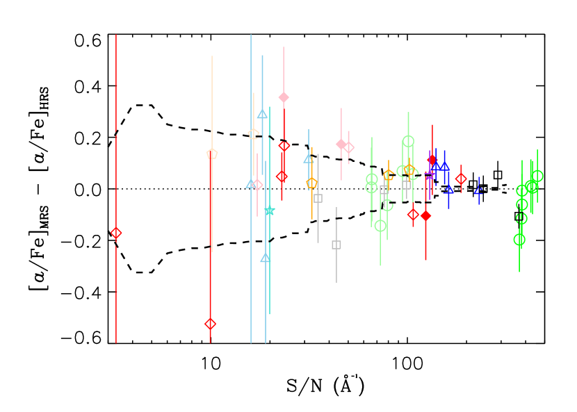
Figure 17.— Differences between $\mathrm{[\alpha/Fe]}_{\mathrm{MRS}}$ and $\mathrm{[\alpha/Fe]}_{\mathrm{HRS}}$ vs. signal-to-noise ratio. The error bars are the sum in quadrature of $\delta_{\mathrm{tot}}\mathrm{[\alpha/Fe]}_{\mathrm{MRS}}$ (Eq. 16) and $\delta\mathrm{[\alpha/Fe]}_{\mathrm{HRS}}$ (Eq. 5.3). The dashed line is the average of $\sqrt{(\mathrm{[\alpha/Fe]}_{\mathrm{MRS}}-\mathrm{[\alpha/Fe]}_{\mathrm{HRS}})^{2}-(\delta\mathrm{[\alpha/Fe]}_{\mathrm{HRS}})^{2}}$ in a moving window with a half width of 0.5 dex in S/N. At $\mathrm{S/N}\gtrsim 320$, $\delta\mathrm{[\alpha/Fe]}_{\mathrm{HRS}}$ completely accounts for the total error, and the argument of the square root becomes negative. The symbols, colors, and references are the same as in Fig. 3 except that faded symbols represent measurements from spectra injected with artificial noise.

We also investigate the effect of noise in estimating [$\alpha$/Fe]. We repeat the comparison in Fig. 10 in which the sample is restricted to those stars also observed with HRS. In Fig. 17 we plot the difference between $\mathrm{[\alpha/Fe]}_{\mathrm{MRS}}$ and $\mathrm{[\alpha/Fe]}_{\mathrm{HRS}}$ vs. S/N. In the same figure, we also plot the results from the same stars injected with artificial noise (faded symbols). The dashed line is the scatter about zero in a moving window with a half width of 0.5 dex in S/N, correcting for the error on $\mathrm{[\alpha/Fe]}_{\mathrm{HRS}}$: $\sqrt{(\mathrm{[\alpha/Fe]}_{\mathrm{MRS}}-\mathrm{[\alpha/Fe]}_{\mathrm{HRS}})^{2}-(\delta\mathrm{[\alpha/Fe]}_{\mathrm{HRS}})^{2}}$. At $\mathrm{S/N}\gtrsim 320$, $\delta\mathrm{[\alpha/Fe]}_{\mathrm{HRS}}$ becomes comparable to $\left|\mathrm{[\alpha/Fe]}_{\mathrm{MRS}}-\mathrm{[\alpha/Fe]}_{\mathrm{HRS}}\right|$. Even at $\mathrm{S/N}\sim 10~{}\mathrm{\AA}^{-1}$ (the typical S/N of a one-hour exposure of an RGB star in M31 (catalog )), the average error is $\sim 0.2$ dex, small enough to distinguish between the halo plateau value of $\mathrm{[\alpha/Fe]}\sim+0.3$ and $\mathrm{[\alpha/Fe]}\sim 0.0$.

A Gaussian noise model is a simplified representation of the actual noise model. In reality, the spectral error contains a systematic component, particularly around night sky lines. A thorough noise model is beyond the scope of this article, but we intend to address this issue in future work. In the meantime, the Gaussian noise model gives a good approximation of the abundance precision we expect with lower S/N spectra.

7. Applications

GCs are already well studied at high resolution. MRS abundance measurement is not intended to provide more accurate abundances for GCs. After all, it has only two dimensions of abundance, although future versions may even allow estimates of individual element enhancements, such as Al, O, Na, Mg, Ca, Ti, La, Ba, and Eu. However, the real strength of MRS is to probe large samples at large distances.

Upcoming studies will focus on the metallicities and $\alpha$ enhancements of the dwarf galaxies of the MW and M31 (catalog ). We also intend to explore the differences between the chemical properties of different kinematic components of M31 (catalog ): the cold dSphs, the disrupted satellites and streams, and the hot halo. We intend for the MRS measurements to be a direct test of chemical evolution simulations, such as those of Font et al. (2006).

In exploring these diverse systems, we will need to recognize some shortcomings of the MRS technique. First, we do not model TiO absorption, and we have discarded all stars that show TiO. In future applications, we intend to continue discarding stars with $T_{\mathrm{eff}}<4000$ K due to the complexity of modeling TiO absorption. Second, the errors at the higher metallicity of M71 (catalog ) ($\mathrm{[Fe/H]}=-0.76$, Pritzl et al., 2005) become somewhat large (0.2 dex), though not larger than typical errors for photometric or Ca II triplet-based metallicities. Both problems will affect metal-rich samples such as the inner halo of M31 (catalog ) ($\langle\mathrm{[Fe/H]}\rangle=-0.47$, Kalirai et al., 2006). Finally, samples of very faint stars may require spectral coaddition in bins of $T_{\mathrm{eff}}$ and $\log g$ to achieve S/N ratios high enough to make measurements of $\alpha$ enhancement with precision greater than 0.3 dex. Although enhancements of individual stars would be unrecoverable, coadded spectra would contain enough information to estimate a stellar population’s overall chemical properties.

We have demonstrated that metallicity measurements of medium resolution spectra via spectral modeling approach the accuracy and precision of measurements from HRS. Furthermore, the leverage of a large number of absorption lines from many different elements allows abundance measurement in multiple dimensions. Presently, the method estimates $\alpha$ enhancement, but future versions may provide individual element enhancements. Spectral modeling is superior to spectrophotometric indices, such as the Ca II triplet EW. First, the precision from modeling is comparable or better at the same S/N. Second, modeling requires no empirical calibration. Therefore, the result is not tied to intrinsic parameters (e.g., [Ca/Fe]) of the calibrators. Additionally, modeling is not subject to the range of metallicities of the calibrators. Whereas empirical calibrations to GCs will be inaccurate at $\mathrm{[Fe/H]}\lesssim-2.4$, the MRS method is applicable to arbitrarily low metallicities, which may exist in some of the lowest mass MW satellites (Simon & Geha, 2007). These advantages make medium resolution spectral modeling the only abundance technique that will be able to test theories of hierarchical structure formation through large samples of individual stars at large distances.

Table 7Abundances for Individual Stars

$\alpha$ (2000.0)	$\delta$ (2000.0)	$B$	$V$	$I$	$T_{\mathrm{eff}}$	$\log g$	$\mathrm{[Fe/H]}_{\mathrm{MRS}}$	$\mathrm{[\alpha/Fe]}_{\mathrm{MRS}}$	$\mathrm{[Fe/H]}_{\mathrm{HRS}}$	$\mathrm{[\alpha/Fe]}_{\mathrm{HRS}}$	HRS reference
M13 (catalog )
$16^{\mathrm{h}}40^{\mathrm{m}}52.1^{\mathrm{s}}$	$+36\arcdeg 29\arcmin 25\arcsec$	$17.31\pm 0.04$	$16.64\pm 0.03$	$15.82\pm 0.01$	5336	3.09	$-1.69\pm 0.13$	$+0.33\pm 0.07$	$\cdots$	$\cdots$	$\cdots$
$16^{\mathrm{h}}40^{\mathrm{m}}58.4^{\mathrm{s}}$	$+36\arcdeg 26\arcmin 04\arcsec$	$16.70\pm 0.02$	$16.03\pm 0.01$	$15.17\pm 0.01$	5204	2.80	$-1.86\pm 0.11$	$+0.41\pm 0.05$	$\cdots$	$\cdots$	$\cdots$
$16^{\mathrm{h}}41^{\mathrm{m}}01.6^{\mathrm{s}}$	$+36\arcdeg 28\arcmin 00\arcsec$	$17.37\pm 0.04$	$16.79\pm 0.02$	$15.95\pm 0.01$	5260	3.13	$-1.71\pm 0.12$	$+0.28\pm 0.07$	$\cdots$	$\cdots$	$\cdots$
$16^{\mathrm{h}}41^{\mathrm{m}}02.6^{\mathrm{s}}$	$+36\arcdeg 26\arcmin 16\arcsec$	$15.68\pm 0.01$	$14.92\pm 0.01$	$\cdots$	4965	2.26	$-1.65\pm 0.12$	$+0.22\pm 0.04$	$-1.44\pm 0.05$	$+0.22\pm 0.03$	Cohen & Meléndez (2005a)
$16^{\mathrm{h}}41^{\mathrm{m}}04.8^{\mathrm{s}}$	$+36\arcdeg 27\arcmin 45\arcsec$	$17.48\pm 0.04$	$16.92\pm 0.01$	$16.10\pm 0.01$	5318	3.20	$-1.82\pm 0.12$	$+0.23\pm 0.09$	$\cdots$	$\cdots$	$\cdots$
$16^{\mathrm{h}}41^{\mathrm{m}}05.8^{\mathrm{s}}$	$+36\arcdeg 26\arcmin 30\arcsec$	$17.47\pm 0.04$	$16.86\pm 0.01$	$16.05\pm 0.01$	5379	3.19	$-1.68\pm 0.13$	$+0.27\pm 0.07$	$\cdots$	$\cdots$	$\cdots$
$16^{\mathrm{h}}41^{\mathrm{m}}06.2^{\mathrm{s}}$	$+36\arcdeg 25\arcmin 22\arcsec$	$15.30\pm 0.01$	$14.46\pm 0.01$	$\cdots$	4829	2.02	$-1.65\pm 0.12$	$+0.23\pm 0.04$	$-1.44\pm 0.05$	$+0.17\pm 0.04$	Cohen & Meléndez (2005a)
$16^{\mathrm{h}}41^{\mathrm{m}}06.5^{\mathrm{s}}$	$+36\arcdeg 28\arcmin 14\arcsec$	$14.29\pm 0.01$	$13.25\pm 0.01$	$\cdots$	4522	1.37	$-1.65\pm 0.12$	$+0.11\pm 0.04$	$-1.63\pm 0.06$	$\cdots$	Sneden et al. (2004)
$16^{\mathrm{h}}41^{\mathrm{m}}09.7^{\mathrm{s}}$	$+36\arcdeg 26\arcmin 45\arcsec$	$15.52\pm 0.02$	$14.73\pm 0.01$	$13.79\pm 0.01$	4997	2.19	$-1.67\pm 0.12$	$+0.30\pm 0.04$	$\cdots$	$\cdots$	$\cdots$
$16^{\mathrm{h}}41^{\mathrm{m}}09.9^{\mathrm{s}}$	$+36\arcdeg 27\arcmin 42\arcsec$	$17.31\pm 0.03$	$16.73\pm 0.02$	$15.91\pm 0.01$	5352	3.13	$-1.52\pm 0.14$	$+0.13\pm 0.08$	$\cdots$	$\cdots$	$\cdots$

Note. — Table 7 is published in its entirety in the electronic edition of the Astrophysical Journal. A portion is shown here for guidance regarding form and content.

References

- Allende Prieto et al. (2006) Allende Prieto, C., Beers, T. C., Wilhelm, R., Newberg, H. J., Rockosi, C. M., Yanny, B., & Lee, Y. S. 2006, ApJ, 636, 804
- Anders & Grevesse (1989) Anders, E., & Grevesse, N. 1989, Geochim. Cosmochim. Acta, 53, 197
- Armandroff & Zinn (1988) Armandroff, T. E., & Zinn, R. 1988, AJ, 96, 92
- Barklem & Aspelund-Johansson (2005) Barklem, P. S., & Aspelund-Johansson, J. 2005, A&A, 435, 373
- Barklem et al. (2000) Barklem, P. S., Piskunov, N., & O’Mara, B. J. 2000, A&AS, 142, 467
- Battaglia et al. (2008) Battaglia, G., Irwin, M., Tolstoy, E., Hill, V., Helmi, A., Letarte, B., & Jablonka, P. 2008, MNRAS, 383, 183
- Brown et al. (2003) Brown, T. M., Ferguson, H. C., Smith, E., Kimble, R. A., Sweigart, A. V., Renzini, A., Rich, R. M., & VandenBerg, D. A. 2003, ApJ, 592, L17
- Brown et al. (2006) Brown, T. M., Smith, E., Ferguson, H. C., Rich, R. M., Guhathakurta, P., Renzini, A., Sweigart, A. V., & Kimble, R. A. 2006, ApJ, 652, 323
- Carbon et al. (1982) Carbon, D. F., Romanishin, W., Langer, G. E., Butler, D., Kemper, E., Trefzger, C. F., Kraft, R. P., & Suntzeff, N. B. 1982, ApJS, 49, 207
- Castelli et al. (1997) Castelli, F., Gratton, R. G., & Kurucz, R. L. 1997, A&A, 318, 841
- Castelli & Kurucz (2004) Castelli, F., & Kurucz, R. L. 2004, ArXiv Astrophysics e-prints, arXiv:astro-ph/0405087
- Chapman et al. (2006) Chapman, S. C., Ibata, R., Lewis, G. F., Ferguson, A. M. N., Irwin, M., McConnachie, A., & Tanvir, N. 2006, ApJ, 653, 255
- Cohen et al. (2005) Cohen, J. G., Briley, M. M., & Stetson, P. B. 2005, AJ, 130, 1177
- Cohen & Meléndez (2005a) Cohen, J. G., & Meléndez, J. 2005a, AJ, 129, 303
- Cohen & Meléndez (2005b) Cohen, J. G., & Meléndez, J. 2005b, AJ, 129, 1607
- Demarque et al. (2004) Demarque, P., Woo, J.-H., Kim, Y.-C., & Yi, S. K. 2004, ApJS, 155, 667
- Dutton et al. (2005) Dutton, A. A., Courteau, S., de Jong, R., & Carignan, C. 2005, ApJ, 619, 218
- Faber et al. (2003) Faber, S. M., et al. 2003, Proc. SPIE, 4841, 1657
- Font et al. (2006) Font, A. S., Johnston, K. V., Bullock, J. S., & Robertson, B. E. 2006, ApJ, 646, 886
- Font et al. (2008) Font, A. S., Johnston, K. V., Ferguson, A. M. N., Bullock, J. S., Robertson, B. E., Tumlinson, J., & Guhathakurta, P. 2008, ApJ, 673, 215
- Fulbright (2000) Fulbright, J. P. 2000, AJ, 120, 1841
- Girardi et al. (2002) Girardi, L., Bertelli, G., Bressan, A., Chiosi, C., Groenewegen, M. A. T., Marigo, P., Salasnich, B., & Weiss, A. 2002, A&A, 391, 195
- Gratton & Ortolani (1989) Gratton, R. G., & Ortolani, S. 1989, A&A, 211, 41
- Gratton et al. (1986) Gratton, R. G., Quarta, M. L., & Ortolani, S. 1986, A&A, 169, 208
- Grundahl (1999) Grundahl, F. 1999, in Spectrophotometric Dating of Stars and Galaxies, ed. I. Hubeny, S. Heap, & R. Cornett, ASP Conf. Proc., 192, 223
- Guhathakurta et al. (2006) Guhathakurta, P., et al. 2006, AJ, 131, 2497
- Harris (1996) Harris, W. E. 1996, AJ, 112, 1487
- Hinkle et al. (2000) Hinkle, K., Wallace, L., Valenti, J., & Harmer, D. 2000, Visible and Near Infrared Atlas of the Arcturus Spectrum 3727-9300 A ed. Kenneth Hinkle, Lloyd Wallace, Jeff Valenti, and Dianne Harmer. (San Francisco: ASP) ISBN: 1-58381-037-4, 2000.,
- Kalirai et al. (2006) Kalirai, J. S., et al. 2006, ApJ, 648, 389
- Koch et al. (2008) Koch, A., Grebel, E. K., Gilmore, G. F., Wyse, R. F. G., Kleyna, J. T., Harbeck, D. R., Wilkinson, M. I., & Wyn Evans, N. 2008, AJ, 135, 1580
- Koch et al. (2007) Koch, A., et al. 2007, Astronomische Nachrichten, 328, 653
- Kraft et al. (1998) Kraft, R. P., Sneden, C., Smith, G. H., Shetrone, M. D., & Fulbright, J. 1998, AJ, 115, 1500
- Kupka et al. (1999) Kupka, F., Piskunov, N., Ryabchikova, T. A., Stempels, H. C., & Weiss, W. W. 1999, A&AS, 138, 119
- Kurucz (1992) Kurucz, R. L. 1992, Revista Mexicana de Astronomia y Astrofisica, vol. 23, 23, 45
- Kurucz (1993) Kurucz, R. L. 1993, Physica Scripta Volume T, 47, 110
- Lee et al. (2007) Lee, Y. S., et al. 2007, ApJ, submitted, ArXiv e-prints, 710, arXiv:0710.5645
- Mishenina et al. (2003) Mishenina, T. V., Panchuk, V. E., & Samus’, N. N. 2003, Astronomy Reports, 47, 248
- Olszewski et al. (1991) Olszewski, E. W., Schommer, R. A., Suntzeff, N. B., & Harris, H. C. 1991, AJ, 101, 515
- Peterson et al. (1993) Peterson, R. C., Dalle Ore, C. M., & Kurucz, R. L. 1993, ApJ, 404, 333
- Preston (1961) Preston, G. W. 1961, ApJ, 134, 633
- Pritzl et al. (2005) Pritzl, B. J., Venn, K. A., & Irwin, M. 2005, AJ, 130, 2140
- Ramírez & Meléndez (2005) Ramírez, I., & Meléndez, J. 2005, ApJ, 626, 465
- Ramírez & Cohen (2002) Ramírez, S. V., & Cohen, J. G. 2002, AJ, 123, 3277
- Robertson et al. (2005) Robertson, B., Bullock, J. S., Font, A. S., Johnston, K. V., & Hernquist, L. 2005, ApJ, 632, 872
- Rutledge et al. (1997) Rutledge, G. A., Hesser, J. E., & Stetson, P. B. 1997, PASP, 109, 907
- Sandage & Wildey (1967) Sandage, A., & Wildey, R. 1967, ApJ, 150, 469
- Searle & Zinn (1978) Searle, L., & Zinn, R. 1978, ApJ, 225, 357
- Shetrone et al. (2001) Shetrone, M. D., Côté, P., & Sargent, W. L. W. 2001, ApJ, 548, 592
- Shetrone et al. (2003) Shetrone, M., Venn, K. A., Tolstoy, E., Primas, F., Hill, V., & Kaufer, A. 2003, AJ, 125, 684
- Simon & Geha (2007) Simon, J. D., & Geha, M. 2007, ApJ, 670, 313
- Sneden (1973) Sneden, C. A. 1973, Ph.D. Thesis, The University of Texas at Austin
- Sneden et al. (2004) Sneden, C., Kraft, R. P., Guhathakurta, P., Peterson, R. C., & Fulbright, J. P. 2004, AJ, 127, 2162
- Sneden et al. (1994) Sneden, C., Kraft, R. P., Langer, G. E., Prosser, C. F., & Shetrone, M. D. 1994, AJ, 107, 1773
- Sneden et al. (1992) Sneden, C., Kraft, R. P., Prosser, C. F., & Langer, G. E. 1992, AJ, 104, 2121
- Sneden et al. (1997) Sneden, C., Kraft, R. P., Shetrone, M. D., Smith, G. H., Langer, G. E., & Prosser, C. F. 1997, AJ, 114, 1964
- Sneden et al. (2000) Sneden, C., Pilachowski, C. A., & Kraft, R. P. 2000, AJ, 120, 1351
- Sohn et al. (2007) Sohn, S. T., et al. 2007, ApJ, 663, 960
- Suntzeff (1981) Suntzeff, N. B. 1981, ApJS, 47, 1
- VandenBerg et al. (2006) VandenBerg, D. A., Bergbusch, P. A., & Dowler, P. D. 2006, ApJS, 162, 375
- Venn et al. (2004) Venn, K. A., Irwin, M., Shetrone, M. D., Tout, C. A., Hill, V., & Tolstoy, E. 2004, AJ, 128, 1177
- White & Rees (1978) White, S. D. M., & Rees, M. J. 1978, MNRAS, 183, 341