The White Mountain Polarimeter Telescope and an Upper Limit on CMB Polarization

Abstract

The White Mountain Polarimeter (WMPol) is a dedicated ground-based microwave telescope and receiver system for observing polarization of the Cosmic Microwave Background. WMPol is located at an altitude of 3880 meters on a plateau in the White Mountains of Eastern California, USA, at the Barcroft Facility of the University of California White Mountain Research Station. Presented here is a description of the instrument and the data collected during April through October 2004. We set an upper limit on $E$-mode polarization of 14 $\mu\mathrm{K}$ ($95\%$ confidence limit) in the multipole range $170<\ell<240$. This result was obtained with 422 hours of observations of a 3 $\mathrm{deg}^{2}$ sky area about the North Celestial Pole, using a 42 GHz polarimeter. This upper limit is consistent with $EE$ polarization predicted from a standard $\Lambda$-CDM concordance model.

1 Introduction

Polarization of the Cosmic Microwave Background (CMB) results from Thomson scattering of CMB photons from local quadrupolar temperature anisotropies during last scattering. Measurements of CMB polarization promise to help to constrain cosmological models, as discussed in, for example, Hu & White (1997). To date, detections of $E$-mode CMB polarization have been reported by DASI (Kovac et al., 2002; Leitch et al., 2005), CBI (Readhead et al., 2004), CAPMAP (Barkats et al., 2005), BOOMERanG (Montroy et al., 2006), WMAP (Page et al., 2007), and MAXIPOL (Wu et al., 2007).

The White Mountain Polarimeter (WMPol) is a ground-based telescope and receiver system designed to observe CMB polarization. This article describes the WMPol instrument and the observing site, including systems used to control WMPol remotely and monitor the weather. Also presented is a summary of the data collected during 2004 and the data analysis methods and results.

2 WMPol Instrument

The WMPol instrument, consisting of a microwave telescope and receiver, is located at an altitude of 3880 meters in the White Mountains east of Bishop, California at longitude 118°14′19″W, latitude 37°35′21″N. The University of California White Mountain Research Station (WMRS) operates the Barcroft Facility, which includes the Barcroft Observatory where the telescope is located. WMPol was installed in the observatory in September 2003 and a concerted data taking effort ran from April to October 2004.

2.1 Telescope

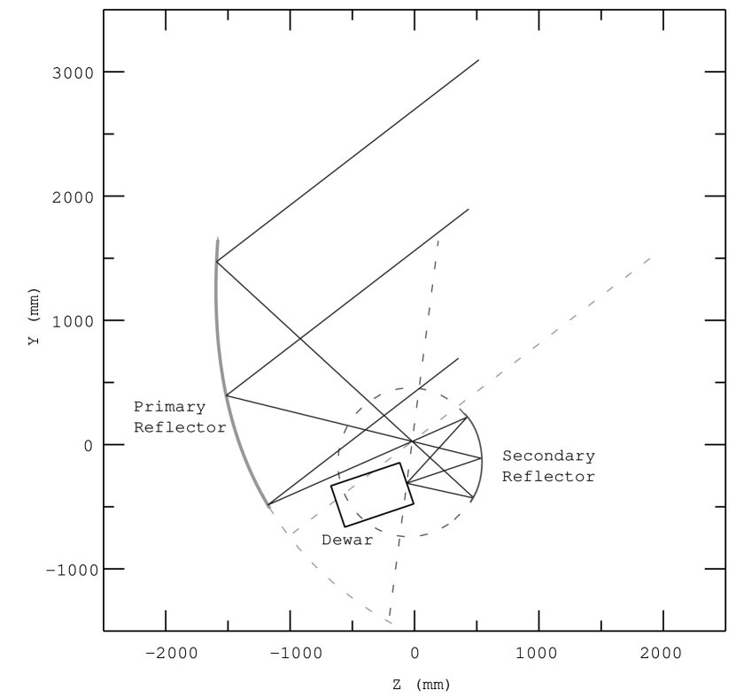
Figure 1: Optical design of WMPol telescope. The primary reflector (with its parent parabola), the secondary reflector (with its parent ellipsoid), and the dewar are shown. Radiation from the sky is focused by the primary at the common focal point of the primary and secondary (the origin of the plot) and then focused by the secondary at the phase center of the central horn in the dewar.

The WMPol telescope is an off-axis Gregorian telescope with a 2.2-meter diameter parabolic primary. The telescope design, which obeys the Dragone-Mizugutch condition (Dragone, 1978; Mizugutch, Akagawa, & Yokoi, 1976), is similar to that of BEAST, a telescope dedicated to mapping CMB temperature anisotropies (Childers et al., 2005; Figueiredo et al., 2005; Meinhold et al., 2005; Mejía et al., 2005; O’Dwyer et al., 2005; Donzelli et al., 2006), and uses identical aluminum coated carbon fiber reflectors. Figure 1 shows the optical design including the primary, 0.9-meter diameter ellipsoidal secondary, and the dewar that houses the receivers.

The WMPol telescope is mounted on top of a table that rotates in azimuth. The table is attached to a shallow cone that rests on four smaller conical roller bearings. A motor drives the motion in azimuth by rotating one of the roller bearings through a harmonic reducing gear. This table, as described in Meinhold et al. (1993), was used previously to observe CMB temperature anisotropies from the South Pole.

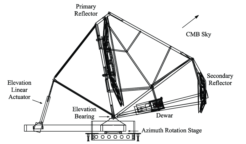
Figure 2: Drawing of the WMPol telescope with primary, secondary, dewar, and frame shown.

The telescope itself consists of a section that is mounted directly to the table and another section (held by two bearings) that can move in elevation via a linear actuator. The motors for the azimuth drive and elevation actuator are controlled by a dual-axis motion controller that uses relative encoders for feedback and linear servo amplifiers to drive the motors. Removable switches that limit the motion in azimuth to approximately $\pm 5\arcdeg$ were installed to prevent the possibility of damage to the telescope during remote operation. Figure 2 shows the major elements of the telescope.

The position of the telescope in azimuth and elevation is measured by two 16-bit absolute encoders and tilt is measured by two biaxial clinometers, one with a $\pm 10\arcmin$ range and the other with a $\pm 10\arcdeg$ range. In practice, tilt of the telescope can be controlled to within $\sim\pm 2\arcmin$ over the full $360\arcdeg$ azimuth range of motion.

A PC operates the telescope using code written at UCSB. This code controls the telescope motion and reads position and tilt, takes data through a data acquisition card, operates an optical CCD camera, and controls the calibrator as described in Section 4.5 below. Temperature at two points on each reflector is measured using AD590 ambient temperature sensors.

A great deal of effort went into arranging the power connections to the telescope to suppress noise. Separate isolated linear power supplies are used for the receiver and housekeeping electronics and isolation transformers are used on the computer and receiver power supplies. All telescope power comes from a dedicated ferroresonant uninterruptible power supply, or FERRUPS, and separate cables from the FERRUPS bring power to the telescope drive, telescope computer, and receiver. In addition, the linear servo amplifiers are installed on the azimuth and elevation drives specifically to reduce noise.

2.2 Receiver

The microwave receiver system consists of two continuous comparison polarimeters, one in Q-band ($38-46$ GHz) and one in W-band ($82-98$ GHz) plus a W-band radiometer to measure CMB temperature anisotropies. Figure 3 shows the Q-band and W-band filter bands. The front ends of the receivers are contained inside an evacuated vacuum vessel (dewar) and cooled to below 30 K with a two-stage Gifford-McMahon cycle cryogenic refrigerator using helium as the refrigerant. The receivers view the optics through a 10.8 cm diameter $50\,\mu$m thick mylar vacuum window which was measured to have a radiometric temperature of 3 K in W-band. A 0.3 cm thick sheet of microwave transparent extruded polystyrene (“blue foam”) is attached to the radiation shield inside the dewar between the receivers and the window to block infrared radiation and thus reduce the heat load on the cold stage.

The receiver topology is similar to the design of the NASA WMAP radiometers (Jarosik et al., 2003) and the baseline design for the Low Frequency Instrument (LFI) for ESA-Planck (Seiffert et al., 2002). The polarimeters are designed to measure the (local - i.e. in the telescope reference frame) $Q$ Stokes parameter, or $\langle E^{2}_{hor}\rangle-\langle E^{2}_{ver}\rangle$, while the anisotropy measuring radiometer is designed to measure the temperature difference between two points on the sky separated by $\sim 1^{\circ}$.

As shown in Figure 4, conical corrugated scalar feed horns (Villa, Bersanelli, & Mandolesi, 1997, 1998) couple the microwave radiation from the telescope to the polarimeters. As is the case for other CMB polarization measurements, WMPol calls for feed horns with a highly symmetric radiation pattern, extremely low cross-polarization, low loss over a relatively large bandwidth ($\sim 20\%$ in our case), and optimal sidelobe rejection. The optimized electromagnetic design for the W-band feeds required throat section grooves $\sim 0.13$ mm thick and $\sim 1.5$ mm deep. To meet these requirements, the W-band feeds were manufactured via electroforming, with a measured deviation from the theoretical mandrel dimensions of less than 10 microns. The larger physical size of the Q-band feeds and their corrugations made it possible to machine the horns from an aluminum cylinder rather than electroforming. The main design parameters and measured performances for the WMPol feeds are shown in Table 1. Figure 5 displays the return loss of the Q-band and W-band feeds.

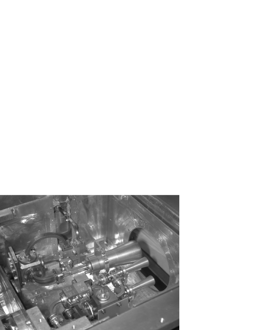
Figure 6: View inside the dewar. The W-band polarimeter horn (top, small horn) is aligned with the optical axis of the telescope and the two W-band horns underneath are for the W-band anisotropy radiometer. The Q-band polarimeter horn is tilted $4\arcdeg$ towards the W-band polarimeter horn due to the curvature of the focal plane when off of the optical axis.

For each polarimeter, the radiation from a horn feeds into an orthomode transducer (OMT). The OMTs use an asymmetric design with specifications as reported in Table 2. From the OMT, the two polarizations are split and go into the two inputs of a $180$ degree hybrid coupler. The two outputs of the $180$ degree hybrid lead to cryogenic amplification with High Electron Mobility Transistor (HEMT) monolithic microwave integrated circuit (MMIC) amplifiers and then more amplification outside of the dewar, plus bandpass filtering in the case of the W-band polarimeter, before leading to the second 180 degree hybrid. The path between the two hybrid couplers is phase-sensitive and $180\arcdeg$ phase switches are installed to facilitate changing one of the path lengths by $\lambda/2$ at a modulation frequency of $100-250$ Hz. Adjustable attenuators are also installed in the phase-sensitive paths to match the gain of the two paths and thin brass shims (approximately $\lambda/40$ or 0.23 mm for Q-band and 0.10 mm for W-band) are used to match the phase lengths of the two paths. The outputs of the second hybrid go to square-law detector diodes. The bandpass filters for the Q-band receiver are placed between the hybrid and the detector diodes. The diode outputs are fed into a $\times 100$ gain differential amplifier before going to a lock-in amplifier referenced to the phase modulation frequency. The purpose of differencing the detector diodes is to improve the 1/$f$ noise performance of the instrument. Finally, the output of the lock-in goes to an ideal integrator and the data acquisition card in the telescope computer. The individual diode signal levels after $\times 100$ gain are also recorded. These DC levels do not benefit from the improved 1/$f$ performance that differencing provides and do not go to a lock-in amplifier. However, these measurements were found to be very helpful for calibration and measuring sky temperature as described further below. Table 3 identifies the sources of various elements of the polarimeters and Figure 6 is a photograph of the inside of the dewar.

The W-band CMB temperature anisotropy radiometer is similar to the polarimeters except that two horns feed into the first hybrid coupler and the outputs of the second hybrid coupler feed into a single pole double throw PIN switch modulated at 5 kHz which then feeds a square law detector diode. Phase sensitive detection at this modulation frequency provides a signal that is proportional to the temperature difference between the two points on the sky that the horns view. Due to space limitations and other considerations, adjustable attenuators are not used in the phase sensitive paths; instead, the gains are matched through small changes in the bias voltages.

All the radiometer electronics and the microwave components outside of the dewar are contained in a contiguous aluminum shield. To reduce noise, the dewar is electrically isolated from the telescope frame except for two ground connections. One ground connection goes from the dewar to the cryogenic refrigerator cold head and the helium compressor through the compressed gas lines and electrical cable that connect the cold head to the compressor. Another ground connection from the dewar to the radiometer power supply ground ensures that the dewar ground connection is not severed if the cryocooler power cable is disconnected from the wall.

The noise temperatures of the Q-band and W-band polarimeters are measured using manual calibrations of the non-differenced DC channels. The resulting Q-band noise temperature is 127 K and the W-band noise temperature is 120 K. The high noise temperature, especially for the Q-band system, is mostly due to the quality of amplifiers that were available to us at the time that the receivers were assembled, tested, and deployed. As the measured room temperature losses due to the OMT and hybrid coupler before the cryogenic amplifiers are less than 0.5 dB for Q-band and 1.5 dB for W-band, the maximum contribution to the polarimeter noise temperature due to front end losses, assuming the polarimeters are at a physical temperature of 30 K, is 4 K for Q-band and 12 K for W-band. The W-band anisotropy measuring radiometer failed soon after the telescope was installed in the Barcroft Obsevatory and repeated attempts to discover the problem have not been successful. Table 4 is a list of receiver noise temperatures, effective bandwidths, and sensitivities for the Q and W polarimeters.

During the testing and commissioning of the instrument, it was found that the polarized offsets were rather high ($\sim 26$ K) which limited the amount of gain that the polarimeter output could be multiplied by before going to a data acquisition channel. The offset is due to a change in DC signal out of the diodes when the phase switches are in different states. We believe the origin of the offset is the asymmetry between the two output arms of the OMT, which is not correctable in our radiometer design. A circuit was designed and successfully implemented to remove the offset before sending the signal to the data acquisition system.

3 The Barcroft Observatory

Although microwave atmospheric emission is known to be not significantly polarized (Hanany & Rosenkranz, 2003), the choice of a suitable observing site is mandatory to optimize the data taking efficiency, reduce systematic effects and avoid large baseline drifts. The WMRS Barcroft Facility provides an excellent site for CMB observations. The addition of a remote control system to operate WMPol and weather monitoring at the Barcroft Observatory improved our ability to collect data safely and efficiently.

3.1 Sky Temperature

Marvil et al. (2006) and a previous study of atmospheric emission at Barcroft (Bersanelli et al., 1995) show low water vapor content at the Barcroft Facility, with observed limits as low as $\sim 0.2$ mm. Assuming precipitable water vapor content in the range $0.2-6$ mm and calibrating the atmospheric emission model of Danese & Partridge (1989) with more recent data, we expect zenith atmospheric (sky) temperatures at the centers of the WMPol bands in the ranges of $9-12$ K at 43 GHz and $7-16$ K at 90 GHz. It should be noted that the atmospheric emission spectrum in the $40-45$ GHz range, dominated by O₂ broadened line complex, is extremely steep so that the tail of the band can contribute significantly to the zenith sky temperature (see Figure 3 for the WMPol Q-band filter band).

The sky temperature is measured with sky dips. For WMPol, the sky dips are scans in elevation from $32\arcdeg$ to $48\arcdeg$ at azimuth $0\arcdeg$, which give the zenith sky temperature after fitting to the model

$$T_{\mathrm{antenna}}=T_{\mathrm{system}}+\frac{T_{\mathrm{zenith}}}{\sin(\theta)}$$ (1)

where $\theta$ is the elevation angle. During the observing campaign, the measured mean zenith sky temperature was $(9\pm 0.2)$ K and $(10\pm 0.6)$ K for Q-band and W-band respectively with measurements ranging from $8-11$ K for Q-band and $9-15$ K for W-band. These values agree well with the predicted values and measurements from Marvil et al. (2006), Childers et al. (2005), and Bersanelli et al. (1995).

3.2 Remote Control System

We considered it quite advantageous to be able to operate the telescope remotely. In order to facilitate remote operation and data collection a number of elements were installed in the observatory to enable monitoring and control of the telescope.

The core of the remote control system is a Stargate automation system. The Stargate has the capability to control X10 (i.e. on/off signals sent over power lines) devices and on-board mechanical relays as well as read digital and analog inputs. The Stargate can accept commands by phone line, internet, or computer via a serial port. The X10 and mechanical relays are used to turn on and off (or power cycle to reset, as needed) the computers and other elements of the telescope.

Another key element of the remote control system is the ability to communicate with and operate the computers in the observatory from other locations. This is achieved by using the Remote Administrator (Radmin) software. Radmin allows for control of the computers at the observatory from the Barcroft station and also from Santa Barbara and potentially anywhere with an internet connection.

For remote operation, it is important to be able to monitor the weather so that the telescope may be protected by closing the observatory shutter in case of high winds or precipitation. As described in Section 3.3, a weather station and a web camera (pointed towards north) are used to monitor sky and weather conditions. The weather station data and camera images are archived every ten minutes and downloaded to a web site at least every half hour for easy monitoring. We also have the ability to view the web camera live.

The optical CCD camera installed on the telescope to assist with pointing reconstruction can be used to monitor cloud conditions at night by checking whether or not Polaris is visible. The CCD camera is also sensitive to clouds during the day.

While it is critical for remote operations to maintain communication with the observatory, the location of the Barcroft Facility and potential for rough weather makes communication a challenge. WMRS has installed two systems to connect to the internet, a satellite connection and a wireless T1 connection through radios at the observatory, White Mountain peak (longitude 118°15′17″W, latitude 37°38′04″N, altitude 4342 meters), and the WMRS Owens Valley Lab, Bishop, CA. We also installed a cell phone base station with our cell phone line connected to the Stargate system. During the first campaign of data taking, lightning and other extreme weather conditions caused some communications outages but, fortunately, no damage to the telescope was suffered during these incidents. As more experience is gained with the communications infrastructure, it is expected to be more reliable.

Another potential issue is power outages due to inclement weather. All the critical elements in the observatory are on FERRUPS for protection and short term power. A planned upgrade to put the shutter control on a UPS and have the shutter close automatically if there is a loss of power would resolve this issue.

3.3 Weather Monitoring

To help protect the WMPol telescope from inclement weather and in order to aid data selection, a commercially available weather station and USB web camera were installed at the Barcroft Observatory. The weather station has the ability to measure temperature, relative humidity, barometric pressure, wind speed and direction, and solar irradiance. Relative humidity in conjunction with the web camera during the day and a CCD camera used for imaging of stars during the night are used to determine the onset of bad weather. To avoid damage to the telescope, the shutter was closed and data taking suspended if inclement weather was imminent or if the average wind speed exceeded 20 mph (8.9 m$\cdot\mathrm{s}^{-1}$) and/or wind gusts exceeded 30 mph (13 m$\cdot\mathrm{s}^{-1}$).

During the April through October 2004 observing campaign, the mean temperature was $3.3\arcdeg$C with an average daily temperature swing of approximately $8\arcdeg$C and the wind speed was lower than our damage-avoidance threshold 93 percent of the time. Marvil et al. (2006) give a more detailed analysis of the Barcroft Observatory weather station data

The web camera images were obtained every 10 minutes and were rated by eye. During the observing campaign, the sky was “Clear,” corresponding to a cloudless period, $46\%$ of the time and “Partly Cloudy,” indicating some scattered clouds, $30\%$ of the time. Periods that were rated “Mostly Cloudy” ($15\%$ of the time) or “Overcast” ($9\%$ of the time) were considered to be times when the weather conditions would not result in useful radiometer data.

4 Observing Campaign

After the telescope was installed in the Barcroft Observatory, Winter 2003-04 was spent commissioning and testing the telescope. We define 2004 April 23 as the official beginning of the observing campaign which ended on 2004 October 17 with the first winter storm of the year and the scheduled seasonal closure of the Barcroft Facility.

4.1 Data Acquisition

During the 178-day campaign, data were recorded during 2169 hours, or just over half of the available time. Table 5 describes the observing time lost due to various issues. Inclement weather, including precipitation and high wind speed, was a major factor and the Stargate automation system was damaged on multiple occasions, we believe due to lightning, causing a great deal of down time. Several levels of surge protection were added to the Stargate during the observing campaign but the seasonal lightning storms ended before it could be determined whether this solved the problem.

The cryogenic refrigerator used to cool the front ends of the radiometers also halted data collection for two reasons. First, the cold end of the refrigerator is known to have a mechanical problem that slightly reduces performance and seems to cause the cooler and dewar to warm up on its own after about fourteen days of continuous operation. In order to recycle the system, the inside dewar temperature has to be brought up all the way to ambient temperature ($\gtrsim 280$ K) before cooling down again; this process requires approximately 24 hours. The other reason for data loss was overheating of the refrigerator’s helium compressor during the middle of the day during summer. The compressor is liquid-cooled with a fan plus radiator to draw heat away from the compressor motor. A thermal cutout prevents damage due to overheating. During winter, a $50-50$ water-antifreeze (ethylene glycol) mix is used to prevent the coolant from freezing during times when the compressor is shut down. This mix has reduced thermal properties as compared to pure water and is not sufficient to transfer heat during midday from the compressor motor in the increased summer temperature conditions. Once this issue was discovered, replacing the anti-freeze mix with distilled water solved the problem.

4.2 Pointing Reconstruction

In order to determine our pointing, we used the Moon and stars to align the optical CCD camera (approximate field of view of $2\fdg 7\times 2\fdg 0$) with the radiometric channels. The size of each CCD camera image pixel, $15\arcsec\pm 1\arcsec$, was determined by observing known stars fields. Observations of the Moon were used to find the central pixel positions of the radiometers in the CCD camera. Subsequent observations of the pixel position of Polaris in the CCD camera allowed us to calculate any offset between the polarimeters and the position of the telescope as defined by the encoders. We estimate our pointing error to be $\pm 3\arcmin$ for the Q-band polarimeter and $\pm 2\arcmin$ for the W-band polarimeter. This pointing error is a small fraction of the beam size. To verify that there were no changes in the pointing on a day-to-day basis, CCD camera images were recorded at all times at a rate around one per minute. In addition we spent 1200 seconds each night of observation staring at Polaris and $\lambda$ Ursae Minoris at approximately 7:00 UT to build up a data base to reveal any changes in the pointing of the telescope or CCD camera.

4.3 Observing Strategy

WMPol used a constant elevation scan strategy, similar to the strategies employed by PIQUE (Hedman et al., 2001, 2002), COMPASS (Farese et al., 2003, 2004), and CAPMAP (Barkats et al., 2005). The telescope maintained an elevation of $37\fdg 6$ while scanning the sky in azimuth $\pm 45\arcmin$ about the North Celestial Pole (NCP) with a period of 9.5 seconds. An advantage of this strategy is that the atmospheric contribution remains nearly constant over short time intervals. Sky rotation allows the telescope to observe a circular region on the sky centered on the NCP. The useful region of the sky observed has an area of 5.5 $\mathrm{deg}^{2}$ in the Q-band polarimeter channel and 1.1 $\mathrm{deg}^{2}$ for the W-band polarimeter channel. The larger coverage area of the Q-band polarimeter is due to a $54\arcmin\pm 1\arcmin$ offset of the Q-band beam from the optical axis, the value of which was determined by observations of the Moon with both polarimeters.

WMPol only measures the Stokes parameter $Q^{\prime}$ in the frame defined by the orthomode transducer of the instrument. The sky Stokes parameters $Q$ and $U$, expressed according to IAU convention (IAU, 1974), are related to WMPol measurements by

$$Q^{\prime}\propto Q\cos 2\psi+U\sin 2\psi,$$ (2)

where $\psi$ is the parallactic angle measured from North and increasing through East (i.e. the angle at the intersection between two great circles passing through the observation point, one containing the NCP and the other the WMPol zenith). Due to the WMPol scan strategy, $\psi$ remains constant and approximately equal zero during data acquisition. So, in the absence of noise, Equation (2) allows us to interpret $Q^{\prime}\simeq Q$. Due to the choice of this scan strategy, WMPol measurements of $U$ Stokes parameter are negligible and are not considered during further analysis.

4.4 Beam Determination

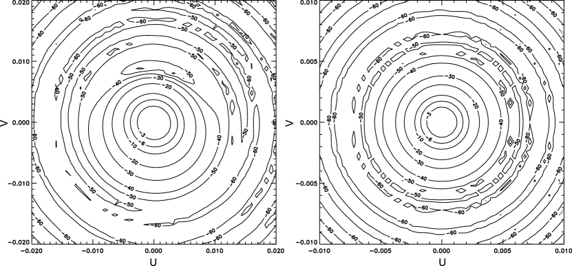
Figure 7: Contour plots of beam models for the Q-band (left) and W-band (right) polarimeters. The axes are dimensionless direction cosines given by $u=\sin\theta\cos\phi$ and $v=\sin\theta\sin\phi$, where $\theta$ and $\phi$ are spherical coordinate angles with respect to the maximum beam response. However, $u$ and $v$ are well approximated by radians for such small angles. The first three contours correspond to -3,-6, and -10 dB below the peak. Note the low level asymmetry (coma lobe) of the off-axis Q-band feed.

The beam sizes of the radiometers on the sky after passing through the optics were modeled using GRASP8. Geometrical optics with geometrical theory of diffraction was used for the secondary reflector, while for the primary reflector physical optics was applied. The geometry was analyzed in transmitting mode (i.e. from feed to sky). In the calculations, far field effects were neglected at the feed level as the feed aperture is only about $4.5\lambda$ and the secondary reflector is at the far field of the feeds. Gaussian beam models of the feeds for both Q-band and W-band were used with modeled FWHM beam sizes of $19.4$ degrees at 41.5 GHz and $19.3$ degrees at 92.5 GHz. Each beam was calculated using a regular (u,v) grid centered on each beam peak in the range (-0.02, 0.02) at 41.5 GHz and (-0.01, 0.01) at 92.5 GHz, for both u and v, corresponding to $1\fdg 15\times 1\fdg 15$ and $0\fdg 575\times 0\fdg 575$ on the sky. Figure 7 shows contour plots of the beam models for the polarimeters. To characterize each beam, an elliptical Gaussian fit of the beam in the whole angular region of calculation was obtained. The modeled characteristics are reported in Table 6 with expected beam sizes (average FWHM) of the Q-band and W-band polarimeters of $18\farcm 8$ and $8\farcm 5$ respectively.

Measurements of the actual beam size were accomplished using the Moon and Tau A. A least squares fit between the observations and the source convolved with a Gaussian beam was used to determine the beam size. The measured FWHM beam size of the Q-band polarimeter is $24\arcmin\pm 3\arcmin$ based on observations of Tau A, as shown in Figure 8. This result is similar to the $22\arcmin\pm 2\arcmin$ quoted in Childers et al. (2005). Presumedly due to 1/$f$ issues, Tau A was not detected with the W-band channel but, by using Moon observations and a model for the Moon as given by Keihm (1984), a FWHM beam size of $12\arcmin\pm 3\arcmin$ was found.

4.5 Calibration

Calibration of the receiver was accomplished with multiple techniques. A manual calibration of the non-differenced channels of the polarimeters was performed by recording the radiometer signals while an ECCOSORB ambient temperature load was placed in front of the radiometers and comparing to the signal levels when viewing the sky.

To calibrate the polarization channels, a grid of 150 $\mu$m diameter copper wires with a 485 $\mu$m spacing was used. This grid was held at an angle of 45 degrees with respect to the dewar window and provided a large polarized signal due to the difference between the temperature of the sky and an ECCOSORB ambient temperature load. As this calibration procedure was manual and required changing the lock-in gain, we also implemented an automated calibrator with a thin dielectric (polypropylene) sheet to perform a relative calibration every 10 minutes. This technique is similar to that described in detail in O’Dell et al. (2002). For each manual calibration of the polarized channels, a transfer standard was calculated and used to convert from the automatic calibrator. This transfer standard, $\alpha$, takes the form

$$\alpha=\frac{|\Delta V_{\mathrm{film}}|}{G|T_{\mathrm{ref}}-T_{\mathrm{sky}}|}$$ (3)

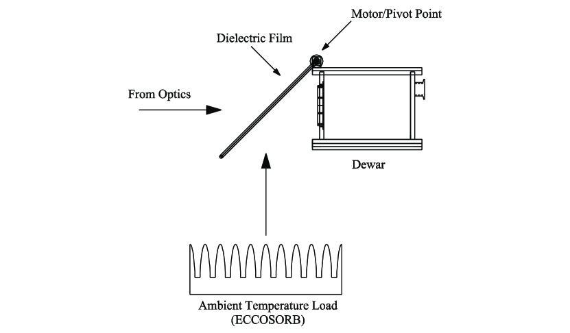
Figure 10: Automatic calibrator. The dielectric sheet is supported by a frame constructed of fiberglass tubing. During a calibration sequence, the dielectric sheet is moved in front of the dewar window as shown and unpolarized radiation from the ambient temperature load and the sky (through the optics) is slightly polarized after reflecting off of or passing through the sheet to the polarimeters. This small polarization signal is due to the difference in the reflection coefficients of the sheet for radiation polarized either parallel or perpendicular to the plane of incidence. After calibration, the frame is rotated away from the polarimeters about the pivot point until it rests on top of the dewar. Limit switches are used to properly position the frame and a digital flag is recorded in the data to identify when calibration sequences occur.

where $\Delta V_{\mathrm{film}}$ is the polarimeter signal offset due to placing the film in front of the dewar, $T_{\mathrm{ref}}$ is the antenna temperature of the ambient reference load, $T_{\mathrm{sky}}$ is the measured mean radiometric sky temperature at elevation $37\fdg 6$, and $G$ is the calibration constant (volts per kelvin) from a manual grid calibration. Figure 9 shows examples of the signal level change in the polarization channels due to the automatic calibration and Figure 10 shows the orientation of the automatic calibrator (or copper wire grid for manual calibration) with respect to the dewar. We estimate the calibration uncertainty on the adopted procedure to be $20\%$.

We verified our Q-band calibration by using Tau A as a target. This source was observed through 7 constant elevation scans during 41 minutes on 2004 September 1. The scans were combined to obtain a Stokes Q map of Tau A at a parallactic angle of $58\fdg 3\pm 0\fdg 4$. The map obtained was compared with Tau A on Q-band maps from the WMAP sky survey (Page et al., 2007; Hinshaw et al., 2007). This procedure allowed us to verify the Q-band automatic calibration within measurement error.

5 Data Analysis

Scientific and housekeeping data were stored in files corresponding to 20 minutes in length. For each file and channel we computed statistical estimators, polarimeter white-noise levels, the weather condition, calibration constants, and other information useful in classifying the data. This procedure allowed us to investigate long time scale behavior of instrument and data, and flag data before producing Stokes Q sky maps.

5.1 Data Selection

Table 7 gives the number of hours of data that were cut from the raw data to create a CMB data set. Data files for times when the telescope was not scanning about the NCP were not used except where data were specifically taken for the purposes of pointing reconstruction, beam size determination, and calibration as discussed below. Also, files shorter than 60 seconds were cut as these files were not expected to contain enough data to be useful. During midday in the late spring and summer the Sun was high enough in the sky to shine directly on the telescope. This not only caused the secondary reflector to heat up by as much as 20°C but also caused the warm components of the polarimeters to heat up to a temperature higher than the servo set point. Changes in signal and gain due to this heating caused the DC signal levels of the polarization channels to exceed the limits of the data acquisition electronics and we labeled these data as “saturated.”

The Q-band and W-band polarization-sensitive channels of each data file were visually inspected. The time-ordered data before and after removing the DC offset on these channels for each half scan (one sweep in azimuth from $-45\arcmin$ to $+45\arcmin$ or the reverse) was examined along with the power spectral density of both channels. The rms of the data after removing the offset was also calculated. Many files that were found to have a rms significantly different from the mean had unusual features in both polarization channels that were presumed to be due to clouds passing through the beam. These files were removed from the data analysis.

After the rms cut, we found that there were data that passed the cut that were collected during bad weather (i.e. web camera image rating equal to “Mostly Cloudy” or “Overcast”) and these data were discarded. Another small amount of data was cut due a cold plate temperature that was too high as a result of the dewar warming up. After cuts, 1574 hours of raw Q-band data and 1208 hours of raw W-band data remained for scientific analysis. These cuts rejected about 27$\%$ of Q-band data and 44$\%$ of W-band data.

5.2 Data Reduction

In order to go from raw time ordered data to calibrated data, the average offset per half scan, auto-calibration sequences, and time domain spikes were removed, the data were calibrated, and binned in azimuth.

Although the signal rms per azimuth bin was consistent with, but slightly higher than, what the instrument sensitivity would predict, calibrated data binned in azimuth did reveal the presence of a scan synchronous signal (SSS). The SSS was sensitive to atmospheric temperature changes and was likely due to thermal emission from the dome into the beam sidelobes of the telescope. A linear regression of calibrated signal as a function of azimuth, performed for each 20 minutes observing period, revealed an average slope of 1 mK/degree in both bands, with variations up to 5 mK/degree/day and 14 mK/degree/day in Q and W bands respectively. Several strategies were tested to minimize SSS contribution, but no reliable model could be established to describe the SSS as a function of ambient temperature, time, or housekeeping data. The SSS removal technique employed involved subtracting from each file a second-order polynomial fit to the calibrated data binned in azimuth. After this procedure, pointing reconstruction was performed and the resulting data was submitted to a maximum likelihood map making algorithm.

5.3 Map Making

We adopted the HEALPix pixelization scheme (Górski et al., 2005), and used the MADCAP package to produce Stokes Q maps (Borrill, 1999). The required inverse time-time noise correlation matrix in the frequency domain was computed as described in Stompor et al. (2002). Noise maps were estimated by computing the difference between two maps, each one produced with half of the available data. Finally, after removing any residual offset by imposing the condition that the map has zero mean, a $\chi^{2}$ test for statistical significance was performed on all the sky and noise maps to check if they were consistent with the null hypothesis, i.e. consistent with no signal.

For the Q-band maps, the null hypothesis was rejected in all the sky and noise maps produced when including data acquired during the day; these maps contain non-stationary residuals from spurious signals due to SSS and the Sun. We applied several masks to select sub-regions in the maps that may be less affected by SSS but the null hypothesis was also rejected in all these sub-regions. For maps obtained using only data acquired during the night, the null hypothesis was accepted in all the sky and noise maps produced. The same result was also obtained when applying masks to select sub-regions in these maps.

For the W-band maps, the situation was different. The W-band data suffered from much higher SSS contamination, and we were unable to determine a filter process that could retain sky signal and remove the SSS. Because of this, these maps were rejected during further analysis.

As a result, the Q-band night time data is the best data set available from WMPol. The Stokes Q map obtained with this subset contains 422 hours of integration, and covers an area of 3 $\mathrm{deg}^{2}$ in a region near the NCP with an effective resolution of $24\arcmin$ FWHM at 42 GHz. The Stokes Q map contains 231 pixels (HEALPix Nside=512, which corresponds to a 6.9 arcmin pixel size), an error of 45 $\mu\mathrm{K}/\mathrm{pixel}$, an rms of 76 $\mu\mathrm{K}$, and thus an error in the mean of 5 $\mu\mathrm{K}$. These 422 hours of data were collected between 2004 July 6 and October 17 and comprise $17\%$ of the possible observing time during this 104 day period. The day time data that were collected during this time period and passed all cuts but were ultimately not included in the final map comprise 378 additional hours.

5.4 Angular Power Spectra

From Monte Carlo simulations, the WMPol EE transfer function was computed assuming a Gaussian beam, the scan strategy, the pixelization scheme, the implemented data reduction pipeline, and the data analysis package. The transfer function is the ratio between the output pseudo angular power spectrum and the corresponding input angular power spectrum. This procedure allowed us to compute the transfer function in the multipole range $100<\ell<500$. The WMPol transfer function is noise dominated for $\ell<120$, it becomes negligible for $\ell>300$, and it takes into account that we have observed only the $Q$ Stokes parameter. Hence WMPol is sensitive to the multipole range $170\lesssim\ell\lesssim 240$. We estimated $EE$ using the PolSpice package (Chon et al., 2004; Szapudi, 2001), which is a method for estimating angular power spectrum from the two-point correlation function and deals with the effects of limited sky, beam smoothing, noise contamination, and inhomogeneous pixel errors. We obtained an upper limit of 14 $\mu\mathrm{K}$ with 95$\%$ confidence level. This upper limit does not include the uncertainties in the Q-band calibration ($20\%$), beam size ($13\%$, which corresponds to $26\%$ uncertainty in beam solid angle), or beam shape, which was assumed to be Gaussian. The Table 8 compares our result to recent CMB polarization measurements, Figure 11 displays the WMPol transfer function and Figure 12 shows our result in the context of the $\Lambda$-CDM concordance model.

6 Conclusion

WMPol was designed, built, and tested at University of California, Santa Barbara and installed in the WMRS Barcroft Observatory to measure CMB polarization in Q-band and W-band. With this telescope and receiver system 2169 hours of data were collected during 2004. The WMPol telescope proved to be robust and a novel remote control system using relatively inexpensive and commercially-available hardware and software was successfully implemented and utilized to operate the telescope over the internet.

WMPol sets an upper limit on $E$-mode polarization of 14 $\mu\mathrm{K}$ ($95\%$ confidence limit, not including calibration and beam uncertainties) in the multipole range $170<\ell<240$. This result was obtained from 422 hours of observations of a Q-band continuous comparison polarimeter on a 3 $\mathrm{deg}^{2}$ sky area near the North Celestial Pole. The reported upper limit is based on a method that estimates the CMB polarization power spectra via the two-point correlation function, and it is consistent with $EE$ polarization predicted from a standard $\Lambda$-CDM concordance model.

Table 1: Design of the WMPol Corrugated Scalar Feed Horns

Parameter	Q-band	W-band
Flare angle (degrees)	7	7
Aperture diameter (mm)	27.16	12.08
Aperture corrugation depth (mm)	1.9	0.88
Aperture corrugation width (mm)	1.45	0.67
Throat diameter (mm)	9.04	2.972
Throat corrugation depth (mm)	3.55	1.51
Throat corrugation width (mm)	1.45	0.13
Number of corrugations	34	37
Corrugation step (mm)	2.17	1.00
Design return loss (dB)	$<-35$	$<-35$
FWHM (degrees)	20	20
Side lobe level(dB)	$<-30$	$<-30$

Table 2: Specifications of the Orthomode Transducers

Parameter	Q-band	W-band
Passband (GHz)	$36.0-43.0$	$85.0-105.0$
VSWR	$1.2:1$ Max	$1.5:1$ Max
Insertion loss (dB)	$0.1$ Max	Not specified
Cross polarization (dB)	$-35$	$-30$

Table 3: Major Elements of the Polarimeters

Device	Source (Q-band)	Source (W-band)
Corrugated scalar feed horns	Univ. of Milan (Italy)	INAF-IASF (Italy)
Orthomode transducers	Custom Microwave	Vertex RSI
Hybrid couplers	QuinStar Technology	Millitech
Cryogenic amplifiers	JPL/UCSB	JPL
Warm amplifiers	Avantek	JPL
Phase switches	Pacific Millimeter Products	Pacific Millimeter Products
Adjustable attenuators	Aerowave	Aerowave
Bandpass filters	UCSB	UCSB
Microwave detector diodes	Pacific Millimeter Products	Pacific Millimeter Products
Differential amplifier	UCSB	UCSB

Table 4: Parameters of the Polarimeters

	$T_{system}$	$\Delta\nu_{eff}$	Sensitivity
Channel	(K)	(GHz)	(mK$\cdot\mathrm{s}^{1/2}$)
Q-band (38-46 GHz)	127	8.0	3.5
W-band (82-98 GHz)	120	12.6	3.0

Table 5: Primary Reasons for Not Taking Data

Issue	Hours
Weather (snow, hail, rain, high wind)	615
Problems with remote control system (often caused by lightning)	955
Scheduled power outages	71
Cryocooler recycling	147
Various glitches (computer/code crashes, cryocooler overheating, etc.)	121
Telescope maintenance and manual calibrations	194
Total lost observing time	2103
Total successful observing time (Raw data)	2169
Total possible observing time	4272

Table 6: WMPol Beam Model Characteristics

Parameter	Q-band	W-band
DIR (dBi)	55.65	62.62
XPD (dB)	39.81	67.01
% DEPOL	0.03	5.6E-05
FWHM X (arcmin)	19.08	8.45
FWHM Y (arcmin)	18.61	8.45
FWHM AVE (arcmin)	18.845	8.45
ELL	1.03	1.0

Note. — DIR is the maximum directivity of the co-polar component. XPD is the cross polar discrimination defined as the ratio between the copolar maximum and the cross polar maximum. % DEPOL is the integrated depolarization factor defined as $(1-\frac{\sqrt{Q^{2}+U^{2}+V^{2}}}{I})\times 100$ where Q, U, V, and I are the Stokes parameters. FWHM X and FWHM Y are the angular resolutions along the major and minor axis of the elliptical fit, ELL is the ellipticity of the -3 dB contour level

Table 7: Cuts of Raw Data

Issue	Q-band (hours)	W-band (hours)
Raw data	2169	2169
Not scanning (testing, calibration, sources)	130	130
Short files (less than 60 s)	$<$ 1	$<$ 1
Saturation (due to Sun)	188	468
RMS cut	173	295
Cold plate temperature	12	6
Weather image	92	62
Total cut	595	961
Data remaining	1574	1208

Table 8: Comparison between recent CMB polarization experiments

Multipole range	Frequency (GHz)	Main $EE$ result	Experiment	Site
$66<\ell<505$	$90$	$<14\ \mu\mathrm{K}$	PIQUE	NJ, USA
			Hedman et al. (2001)
$2<\ell<20$	$26-36$	$<10\ \mu\mathrm{K}$	POLAR	WI, USA
			Keating et al. (2001)
$59<\ell<334$	$90$	$<8.4\ \mu\mathrm{K}$	PIQUE	NJ, USA
			Hedman et al. (2002)
$30\lesssim\ell\lesssim 900$	$26-36$	Detection	DASI	South Pole
			Kovac et al. (2002)
$95<\ell<555$	$26-36$	$<32\ \mu\mathrm{K}$	COMPASS	WI, USA
			Farese et al. (2004)
$400\lesssim\ell\lesssim 1500$	$26-36$	Detection	CBI	Chile
			Readhead et al. (2004)
$640<\ell<1270$	$90$	Detection	CAPMAP	NJ, USA
			Barkats et al. (2005)
$446<\ell<779$	$26-36$	$<7\ \mu\mathrm{K}$	CBI	Chile
$930<\ell<1395$		$<12.8\ \mu\mathrm{K}$	Cartwright et al. (2005)
$1539<\ell<2702$		$<25.1\ \mu\mathrm{K}$
$201<\ell<1000$	$145$	Detection	BOOMERANG	Antarctica
			Montroy et al. (2006)
$2<\ell<6$	$23-94$	Detection	WMAP	L2
			Page et al. (2007)
$151<\ell<693$	$140$	Detection	MAXIPOL	NM, USA
			Wu et al. (2007)
$170<\ell<240$	$42$	$<14\ \mu\mathrm{K}$	WMPol	CA, USA
			This work

Figure 3: Q-band (left) and W-band (right) filter bands. The data show transmission (normalized to input signal) through the filters. The different lines denote each of the filters used in the radiometers.

Figure 4: Schematic of WMPol receiver array. Microwave radiation enters the radiometer through the vacuum window in the dewar (right) where it is fed into corrugated scalar feed horns.

Figure 5: Q-band (left) and W-band (right) feed horn return loss as a function of frequency. Both modeled return loss (dashed lines) and measured performance (solid lines) are reported.

Figure 8: Determination of the Q-band beam size. A least squares fit between observations of Tau A and a point source convolved with a Gaussian beam was used to determine the beam size. The measured FWHM beam size of the Q-band polarimeter is $24\arcmin\pm 3\arcmin$. The number of degrees of freedom is 347, corresponding to 347 HEALPix pixels (3.4 arcmin resolution, nside = 1024) that cover a 1.1 square degrees circular sky area centered on Tau A.

Figure 9: Example of automatic calibration sequence in Q-band (left) and W-band (right), 25 Hz data rate. Placing the dielectric film at a $45\arcdeg$ angle in front of the radiometers creates a relatively small polarization signal that is easily detected.

Figure 11: The WMPol transfer function for Q-band. The transfer function is noisy for $\ell<120$ and it was not computed for $\ell<100$. The multipole $\ell=120$ corresponds to an angular scale of about $1\fdg 5$, which is slightly larger than the radius of the sky area observed. The transfer function becomes negligible for $\ell>300$, which corresponds to an angular scale of about $0\fdg 6$, a value that approaches the Q-band beam size.

Figure 12: WMPol upper limit of 14 $\mu\mathrm{K}$ ($95\%$ confidence limit), on $E$-mode polarization, in the multipole range $170<\ell<240$. This result was obtained with 422 hours of observations of a 3 $\mathrm{deg}^{2}$ sky area near the North Celestial Pole. The predicted angular power spectra $TT$, $TE$, and $EE$ from a $\Lambda$-CDM concordance model are also plotted for illustration.

References

- Barkats et al. (2005) Barkats, D., et al. 2005, ApJ, 619, L127
- Bersanelli et al. (1995) Bersanelli, M., et al. 1995, ApJ, 448, 8
- Borrill (1999) Borrill, J. 1999, preprint (astro-ph/9911389)
- Cartwright et al. (2005) Cartwright, J. K., et al. 2005, Physical Review D, 17, 1901
- Childers et al. (2005) Childers, J., et al. 2005, ApJS, 158, 124
- Chon et al. (2004) Chon, G., et al. 2004, MNRAS, 350, 914
- Donzelli et al. (2006) Donzelli, S., et al. 2006, CMB and Physics of the Early Universe Proceedings, 33
- Dragone (1978) Dragone, C. 1978, The Bell System Technical Journal, 57, 2663
- Danese & Partridge (1989) Danese, L. & Partridge, R. B. 1989, ApJ, 342 604
- Farese et al. (2003) Farese, P. C., et al. 2003, New Astronomy Reviews, 47, 1033
- Farese et al. (2004) Farese, P. C., et al. 2004, ApJ, 610, 625
- Figueiredo et al. (2005) Figueiredo, N., et al. 2005, ApJS, 158, 118
- Górski et al. (2005) Górski, K. M., et al. 2005, ApJ, 622, 759
- Hanany & Rosenkranz (2003) Hanany, S. & Rosenkranz, P. 2003, New Astronomy Reviews, 47, 1159
- Hedman et al. (2001) Hedman, M. M., et al. 2001, ApJ, 548, L111
- Hedman et al. (2002) Hedman, M. M., et al. 2002, ApJ, 573, L73
- Hinshaw et al. (2007) Hinshaw, G., et al. 2007, ApJS, 170, 288
- Hu & White (1997) Hu, W., & White, M. 1997, New Astronomy, 2, 323
- IAU (1974) IAU, 1974, Transactions of the IAU Vol. XVB, 166
- Keating et al. (2001) Keating, B. G., et al. 2001, ApJ, 560, L1
- Keihm (1984) Keihm, S. J. 1984, Icarus, 60, 568
- Kovac et al. (2002) Kovac, J. M., Leitch, E. M., Pryke, C., Carlstrom, J. E., Halverson, N. W., & Holzapfel W. L. 2002, Nature, 420, 772
- Jarosik et al. (2003) Jarosik, N., et al. 2003, ApJS, 145, 413
- Leitch et al. (2005) Leitch, E. M., Kovac, J. M., Halverson, N. W., Carlstrom, J. E., Pryke, C. & Smith, M. W. E. 2005, ApJ, 624, 10
- Marvil et al. (2006) Marvil, J., et al. 2006, New Astronomy, 11, 218
- Meinhold et al. (1993) Meinhold, P. R., et al. 1993, ApJ, 406, 12
- Meinhold et al. (2005) Meinhold, P. R., et al. 2005, ApJS, 158, 101
- Mejía et al. (2005) Mejía, J., et al. 2005, ApJS, 158, 109
- Mizugutch, Akagawa, & Yokoi (1976) Mizugutch, Y., Akagawa, M., & Yokoi, H. 1976, Digest of 1976 AP-S International Symposium on Antennas and Propagation, 2
- Montroy et al. (2006) Montroy, T. E., et al. 2006, ApJ, 647, 813
- O’Dell et al. (2002) O’Dell, C. W., Swetz, D. S., & Timbie, P. T. 2002, IEEE-MTT, 50, 9, 2135
- O’Dwyer et al. (2005) O’Dwyer, I. J., et al. 2005, ApJS, 158, 93
- Page et al. (2007) Page, L., et al. 2007, ApJS, 170, 335
- Readhead et al. (2004) Readhead, A. C. S., et al. 2004, Science, 306, 836
- Seiffert et al. (2002) Seiffert, M., et al. 2002, Astronomy and Astrophysics, 391, 1185
- Stompor et al. (2002) Stompor, R., et al. 2002, Physical Review D, 65, 022003
- Szapudi (2001) Szapudi, I., et al. 2001, ApJ, 548, L115
- Villa, Bersanelli, & Mandolesi (1997) Villa, F., Bersanelli, M., & Mandolesi, N. 1997, ITESRE/CNR Internal Report, 188
- Villa, Bersanelli, & Mandolesi (1998) Villa, F., Bersanelli, M., & Mandolesi, N. 1998, ITESRE/CNR Internal Report, 206
- Wu et al. (2007) Wu, J. H. P., et al. 2006 ApJ, 665, 55