INSTITUT NATIONAL DE RECHERCHE EN INFORMATIQUE ET EN AUTOMATIQUE

Fine-grained parallelization of similarity search between protein sequences
Van Hoa NGUYEN, Dominique LAVENIER N° 6513
April 2008

Abstract: This report presents the implementation of a protein sequence comparison algorithm specifically designed for speeding up time consuming part on parallel hardware such as SSE instructions, multicore architectures or graphic boards. Three programs have been developed: PLAST-P, TPLAST-N and PLAST-X. They provide equivalent results compared to the NCBI BLAST family programs (BLAST-P, TBLAST-N and BLAST-X) with a speed-up factor ranging from 5 to 10.

Key-words: Parallelization, similarity search, indexing, BLAST, GPU, SIMD

Parallélisation à grain fin de la recherche de similarités entre séquences protéiques

Résumé : Ce rapporte présente l’implémentation d’un agorithme de comparaison de séquences protéiques spécialement conçu pour que les parties les plus coûteuses en temps de calcul puissent s’exécuter en parallèle sur des architectures à jeu d’instruction SSE, des architectures multi-coeurs, ou des cartes graphiques de dernières générations. Trois programmes ont été développés : PLAST-P, TPLAST-N et PLAST-X. Ils génèrent des résultats équivalents aux programmes de la famille BLAST (BLAST-P, TBLAST-P et BLAST-X) dévelo- ppés au NCBI. Les facteurs d’accélération (par rapport à BLAST) s’échelonnent de 5 à 10.

Mots-clés : Parallélisation, recherche de similarités, indexation, BLAST, GPU, SIMD

1 Introduction

In genomic, similarity search aims to find local alignments between two DNA or protein sequences, measured by match, mismatch and gap scores. Its objective is to locate regions in DNA or protein sequences having closed relationship. A typical application, for example, is to query a bank with a gene whose function is unknown in order to get some clues for further investigation.

Recent biotechnology improvements in the sequencing area have led to a huge increasing in the size of genomic databases. Genbank [1], for example, contains more than 193 billions of nucleotides (February 2008) and its size is multiplied by a factor ranging from 1.4 and 1.5 every year.

Several algorithms have been proposed to find alignments. One of the first, known as the Smith-Waternam algorithm, has been developed in 1981 [21] to detect local alignments. It uses dynamic programming techniques and has a quadratic complexity. Another one, BLAST, developed in 1990, is currently the reference in the domain [19][18]. This algorithm is based on a powerful heuristic coming from the following observation: an alignment includes at least a word of W characters (called a hit) shares by the two sequences. Thus, instead of exploring a large search space, as it is done in the dynamic programming technique, hits are first used to target small zones of high similarity before computing full alignments.

Many nucleotide search tools, using this heuristics, have been proposed to perform hit detection: MegaBLAST [16], BLAT [14] or PartternHunter [12] [15], for example, include this technique.

These programs (except BLAT) have been mainly designed for scanning genomic databases, that is, given an input sequence (a gene, or a protein), find in the database the other genes or other proteins which share common similarities. There are also used in the context of intensive sequence comparison whose purpose is to compare two genomic databases. In that case, they are not used in an optimal way, leading room for further algorithm improvement.

This report details the results obtained from three programs developed at IRISA: PLAST-P, TPLAST-N and PLAST-X. PLAST stands for Parallel Local Alignment Search Tools by comparison to BLAST (Basic Local Alignment Search Tools). They perform comparison of 2 genomic banks at the protein level by first indexing each bank, and then, by making successive refinements to compute alignments. In addition, hits are found using subset-seeds [3] to optimize memory access.

As in the BLAST family, PLAST-P takes as input 2 protein banks, TPLAST-N takes as input a protein bank and a nucleotide bank, and PLAST-X takes as input two nucleotide banks. In the two last programs, the nucleotide banks are translated into 6 reading frames and the comparison is made using amino acid substitution cost. Different implementations have been designed ranging from pure sequential version to highly parallel version using modern graphics processing units (GPU).

Practically, these programs need to have the input banks in the FASTA format. The alignments are generated following the -m 8 BLAST output format. As these programs are expected to be used in intensive comparison contexts, this format is well suited for automating post processing. Table 1 shows an example of three alignments in this format (-m 8 option). An alignment is summarized on a single line with the following items: contents ID of sequence in bank1 and sequence in bank2, alignment length, position of alignment on the two sequences, E-value and bit score.

	qry. id	sub. id	alig. len.	q. start	q. end	s. start	s. end	bit score
1	P93208	gi0689	249	1	247	1	243	296.3
2	P62261	gi0689	236	2	236	1	233	309.4
3	P30488	gi2750	93	217	305	64	155	43.9

Table 1: Example of BLAST output with option -m 8.

The remainder of this report is organized as follows: In the next section, a brief overview of the BLAST-P algorithm is given. Section 3 presents the PLAST-P algorithm. Section 4 details the sequential version of PLAST-P. Section 5 describes the parallel version of PLAST-P. Section 6 and 7 report results of TPLAST-N and PLAST-X.

2 BLAST-P algorithm

BLAST is one of the most popular bioinformatics tools and is used to run millions of queries every day. A family of BLAST programs has been developed, depending on the type of input. According to these input, the following naming is done: BLAST-P when the query is an amino acid sequence and the database is made of protein sequences; TBLAST-N when the query is an amino acid sequence and the database is made of nucleotide sequences; BLAST-X when the query is a nucleotide sequence and the database is make of amino acid sequences. This section briefly describes the principle of the BLAST-P algorithm. It will help for understanding the difference with the PLAST-P algorithm.

2.1 Context

Generally, in database search, when given a protein sequence, the objective is to extract from a database all the similar sequences, or zones of similarity. The biological motivation of this operation is generally to assign a function to unknown genes or proteins: in a cell, a protein adopts a specific 3D shape related to its sequence of amino acids. This 3D structure is important because the protein function and its interaction with other molecules are determined by this structure. Two proteins with nearly identical 3D shape are assumed to have similar functionalities. Thus, finding similar sequences is correlated to find similar structures and then to similar functionalities.

Furthermore, today (April 2008) there are about 760 genomes being completely sequenced, and there are more than 3600 other ongoing sequencing projects [22]. Now, entire genomes are considered as the main pivot in many bioinformatics research projects. Genes are no longer considered separately. The genes of a same family across multiple species, for example, may represent the abstract object one wants to study. Thus, instead of manipulating sequences with a few thousands of characters (genes), the needs have exploded to processing sequences of a few millions of characters, called intensive computation.

Database search has to explore large genomic banks (hundreds of billions of nucleotides), while intensive computations works on much less data. Suppose, that comparing two strings of respectively $L_{1}$ and $L_{2}$ characters has a complexity of $L_{1}\times L_{2}$. Searching a sequence of size $10^{4}$ over a $10^{10}$ character database has the same complexity as comparing two strings of size $10^{7}$.

In the first case, the problem is I/O bounded: the search time mainly depends on the bandwidth capacity of the system to transfer the database from the disk to the CPU. In the second case, the problem is compute bounded since the search time mainly depends on the computational resources available for computing alignments. The BLAST-P family programs have been primarily designed for scanning large databases. Their use in intensive comparison context is possible, but don’t provide optimal performances.

2.2 Generic algorithm

This section gives an overview of the BLAST family algorithm for searching proteins. We will focus on BLAST-P, but the TBLAST-N and BLAST-X extensions are governed by similar procedures and won’t be detailed.

BLAST-P can be described by the following algorithm when comparing two protein banks referred as bank1 and bank2.

BLAST-P Algorithm
for all sequences in bank1
make index	#stage 0
for all sequences in bank2         // scan of bank2
compute double hits from index	#stage 1
for all double hits
compute ungapped alignment	#stage 2
if score $\geq S_{1}$
compute gapped alignment	#stage 3
if score $\geq S_{2}$
trace-back & display alignment	#stage 4

In the context of intensive genomic computation between bank1 and bank2, bank2 is scanned N times (N is the number of sequences of bank1). From a computational point view, this approach is not efficient since bank2 need to be read a potentially large number of times. Actually, from version 2.2.10 to 2.2.13, the -B N option has been added to search block of multiple sequences. This option allows the user to concatenate all sequences in bank1 into a single one. Thus, the argument of the -B option must be equal to the number of sequences in bank1. Processing multiple sequences in one run can be much faster than processing them separately because bank2 is scanned only one time. From version 2.2.14 to 2.2.17, BLAST-P automatically concatenates several sequences (in bank1) and then compares it with bank2. The concatenated size is about 10,000 amino acids. The execution time is improved, but for processing large database this is still not sufficient.

BLAST-P can be split into 5 different stages (from 0 to 4) which are now described in the next sections.

2.3 The 5 stages of the BLAST-P algorithm

2.3.1 Stage 0: Indexing.

This first stage computes an index structure for each sequence of bank1 using words of W characters [17]. To do this, the sequence is parsed into fixed-length overlapping subsequences of size W. For example, if we suppose W = 3, then, from the following sequence NTHELYSLEISPQ, words are: NTH, THE, HEL, ELY, LYS, YSL, SLE, and so on. These words are called seeds since they are used to generated hits.

To augment the sensibility, BLAST-P computes neighborhood seeds. They are identified by computing a score between pairs of words using substitution costs from a substitution matrix. Pairs having a score greater than a predefined threshold value T are considered as neighborhood seeds. Figure 1 illustrates the identification of neighborhood seeds tacking a threshold value T = 11 (default value of BLAST-P).

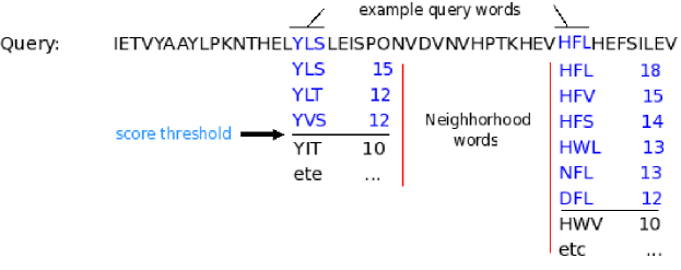
Figure 1: Example of neighborhood seeds with threshold equal to 11.

More formally, two seeds $A_{1},...,A_{i}$ and $B_{1},...B_{i}$ are considered as neighborhood seeds if:

$$\sum_{k=1}^{i}Sub(A_{k},B_{k})\geq T$$

with $Sub(A,B)$ the cost for substituting A by B.

Once neigborhood seeds have been identified, they are are stored into a lookup table acting as an index structure. Typically, seeds of 3 or 4 amino acids are taken (default value of BLAST-P is 3).

2.3.2 Stage 1: Double hit computation

When two seeds coming respectively from the query sequence and the bank sequence match, the seed positions are labeled as a hit. It can be seen as an anchoring point between the two sequences to locate zone of potential alignment.

BLAST-P starts an alignment if two hits are found within a small zone with no gaps. To determine these zones, hits are assigned with a diagonal number. Hits with identical diagonal numbers, and closed to each other, potentially belong to the same ungapped alignment.

BLAST-P detects these pairs of hits thanks to the index previously construct. All the overlapping words of the sequence from the bank are considered and search in the look-up table. Interesting pairs of hits are selected if their distance is smaller than a window size of 40 amino acids.

2.3.3 Stage 2: Ungapped extension

For each pair of hits selected in the previous stage, left and right ungapped extensions are started. This process ignores insertion and deletion events. The aim is to quickly compute a score according to a given substitution matrix. Starting from 0, the score is increased or decreased depending on the substitution cost between successive amino acids. The process start on the right hit and run to the left (to reach the left hit). It stops when the score becomes lower than a predefined threshold value or when it decreases too much. If the left hit has been reached, then a right extension is run.

If the score exceeds a threshold value $S_{1}$, – a constant determined by an external parameter – then the next stage can be started.

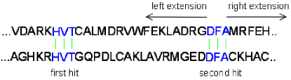
Figure 2: Example about two hits on the same diagonal.

BLAST-P can also be run in one hit mode, where a single hit, rather than two hits, is required to trigger an ungapped extension. This leads to an increase in the number of ungapped extensions performed, increasing runtimes, but improving search accuracy. To reduce the number of hits, a larger value of the neighbor threshold T is typically used when BLAST-P is run in this mode. The original BLAST-P algorithm [19] was using the one hit mode. The double hit optimization was one of the main changes introduced in the 1997 BLAST-P [18].

2.3.4 Stage 3: Gapped extension

In the third stage, the dynamic programming algorithm is used in an attempt to build gapped alignments that passes through ungapped region. A start point is chosen from ungapped alignment, then dynamic programming is used to find the highest-scoring gapped alignment that passes through this point. The gapped alignment algorithm used by BLAST-P differs from Smith-Waterman [21] local alignment. Rather than exhaustively computing all possible paths between the sequences, the gapped scheme explores only insertions and deletions that augment the high-scoring ungapped alignment. After this, a gapped alignment is attempted. The term gapped alignment is referred to the approach used by BLAST-P and local alignment to refer to the exhaustive Smith-Waterman approach.

A gapped alignment stops when the score falls below a drop-off parameter, X. This parameter controls the sensitivity and speed tradeoff: higher the value of X, greater the alignment sensitivity but slower the search process. If the resulting gapped alignment score exceed $S_{2}$ – which is determined from an external E-value cutoff parameter – it is passed to the final stage.

2.3.5 Stage 4: Trace-back & display.

In this stage, the final alignments are constructed and displayed. During the scoring process, the alignment trace-back pathway is recorded so that it can be easily reconstructed. Only alignments that are considered as statistically significant are output. More precisely, only alignments having a score reflecting an expected value greater than a threshold value set by the user are reported.

2.4 Code profiling

In [11] a profiling of the NCBI BLAST-P code has been conducted. It is summarized in the following table.

Task	Percentage of overall time
Find high-scoring short hits	37%
Identify pairs of hits on the same diagonal	18%
Perform ungapped alignment	13%
Perform gapped alignment	30%
Trace-Back and display alignments	2%

Table 2: Average runtime for each stage of BLAST-P algorithm on Genbank non-redundant protein database [11].

In this experiment, the database is the release 113 (August 1999) of GenBank non redundant protein bank and 100 queries have been randomly selected from this bank. The processor is an Intel Pentium 4 cadenced at 2.8 GHz with 1 GByts of main-memory. BLAST-P has been run on the version 2.2.8 with default parameters.

This table shows the percentage of execution time spent on each stage. It can be seen that nearly half of the time is spent in detecting positions where alignments can be started (stage 1). Our approach aims at reducing the time spent during this stage even if the next stages will have to performed more computation. The idea is that computing gapped or ungapped alignments is much more suited for parallelization and that, globally, we should gain on the total execution time.

3 PLAST-P algorithm

3.1 Introduction

An immediate way to speed-up database search is to split the genomic database into N parts on a N-node cluster and to process them separately as it is done with the mpiBLAST implementation [13]. A query sequence is broadcasted and independently processed on each PE before merging the results. The advantages of this parallelization are manifold: access to the data is fast and efficiency is nearly maximal since the communication overhead between the PEs minimal.

For the last 2-3 years, because of the difficulty of increasing clock frequency, processor performance growth has been limited. To keep a high computational power, manufactures now propose chips having several processor cores. These new architectures will be efficient for high performance computation only if codes fit these architectures.

During the last decade, GPUs (graphics Processing Units) have been highly improved by including a large number of specialized processors. The GPUs have many advantages over CPU architectures for processing highly parallel algorithms. They now become a real alternative for deporting very time consuming general purpose computations.

To benefit from these last technologies, we propose a double indexing bank approach allowing both a strong reuse of data and a high potential parallelism on the new generation of multicore processors together with the use of accelerators such as GPU and FPGA.

3.2 PLAST generic algorithm

To avoid the problem of scanning database many times, the two banks are first indexed in the main computer memory before any processing. Through an appropriate index structure, we can point directly to all the identical words (seeds) in both sides of the two banks. If a seed appears $|nb1|$ times in bank1 and $|nb2|$ times in bank2, then there are $|nb1|\times|nb2|$ hits. It means that there are also $|nb1|\times|nb2|$ ungapped alignments to calculate. The PLAST-P algorithm proceeds in 5 successive stages. Stage 0 index the two banks, stage 1 constructs two neighborhood blocks, stage 2 performs ungapped extension, stage 3 computes gapped alignment and stage 4 displays alignments. These stages are described in the following sections.

PLAST-P generic algorithm
	index1 = make index (bank1)	#stage 0
	index2 = make index (bank2)
	for all possible seeds
	construct neighborhood block nb1 from index1	#stage 1
	construct neighborhood block nb2 from index2
	for each subsequence of nb1
	for each subsequence of nb2
	compute ungapped alignment	#stage 2
	if score $\geq S_{1}$
	compute small gapped alignment	#stage 3.1
	if score $\geq S_{2}$
	compute full gapped alignment	#stage 3.2
	if score $\geq S_{3}$
	trace-back & display alignment	#stage 4

3.3 The 5 stages of the PLAST-P algorithm

3.3.1 Stage 0: Bank indexing.

In the PLAST-P algorithm, bank indexing is done using the subset seed concept [8] [9]. Subset seeds have an intermediate expressiveness between spaced seeds [12] and vector seeds [10]. Their main advantage is that they provide a powerful seed definition while preserving the possibility of direct indexing. Here, we use the following subset seed:

A,C,D,E,F,G,H,K,L,M,N,P,Q,R,S,T,V,W,Y

c={C,F,Y,W,M,L,I,V}, g={G,P,A,T,S,N,H,Q,E,D,R,K}

A,C,f={F,Y,E},G,i={I,V},m={M,L},n={N,H},P,q={Q,E,D},r={R,K},t={T,S}

A,C,D,E,F,G,H,K,L,M,N,P,Q,R,S,T,V,W,Y

The index structure of a bank is shown figure 3. All words of length W (seeds) are considered and translated into their corresponding subset seed. For example, the words AQAA, APAA, ASAA are translated to a unique word: AgAA. Then, words having the same subset seed are linked together.

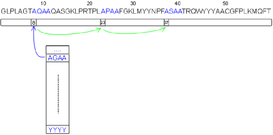
Figure 3: Index structure for storing the positions of the word AGAA.

A look-up table containing all the subset seeds gives a direct access to the linked lists. For each subset seed, its first occurrence in the database is provided.

3.3.2 Stage 1: Neighborhood block building

Hits detected in the first stage are the starting point for computing ungapped alignments. The objective is to be able to rapidly decide if one hit has favorable environment to build an alignment. The index structure gives the position of the W-AA words, allowing to access to the neighboring amino acids for processing ungapped alignments.

In this stage, for all identical seeds, two neighborhood blocks are built: one block (nb1) for bank1 and another block (nb2) for bank2. A block is made of neighborhood amino acids around each seed. Building blocks allow a best reuse of the cache memory when computing ungapped alignment. Figure 4 shows the blocks of subsequences for words AGAA, AGCG and YCFA with four neighborhood amino acids on the left and on the right.

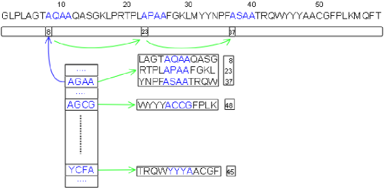
Figure 4: Neighborhood blocks including seeds and 4 characters on their left and right hand side

3.3.3 Stage 2: Ungapped alignment.

For each different seed, we perform $|nb1|\times|nb2|$ ungapped alignments from the two neighborhood blocks previously built. More precisely, for each subsequence in block nb1, we calculate the ungapped score with $|nb2|$ subsequences in block nb2. Unlike BLAST-P, ungapped extension is performed on subsequences of bounded length. Another major difference is that ungapped extension starts as soon as a single hit is identified (BLAST-P requires two hits on the same diagonal and closed to each another before starting an alignment). If the score of the ungapped alignment is greater than a threshold value $S_{1}$, it is passed to the next stage.

According to our experimentations, the computation time of this stage is very important. This part of code is thus a strong candidate for parallelization.

The ungapped algorithm is the following: starting from the first character of seed on both subsequences, the extension runs on the right. It stops when the score becomes lower than a predefined threshold value or when it decreases too much. If the score dose not exceeds a threshold value $S_{1}$ then a left extension is run.

3.3.4 Stage 3: Gapped alignment.

Dynamic programming technique is used to extend ungapped alignments. Actually, this stage is divided into two sub-stages: the first find small gapped alignments (stage 3.1). It aims to limit the searching space of dynamic programming by allowing only a maximal number of gaps. If the score exceeds a threshold value $S_{2}$, the standard dynamic programming procedure is launched (stage 3-2). Experiments have shown that, in many cases, the second step is not done (90%).

The reason why this stage is divided into two parts is that the first one is much more suited for parallelization on hardware accelerator and appears as a good filter before starting a full dynamic programming search.

Most of the time, gapped alignments content more than one ungapped alignment. In such a case, two ungapped alignments are not on the same diagonal. For this reason, sometime, same gapped alignments are recalculated from different ungapped alignments. To avoid this problem, all ungapped alignments belonging to gapped alignments are stored in a structured list. Before starting the computation of a new gapped alignment, we first check if the hit doesn’t belong to ungapped alignment of this list.

In the list, for each ungapped alignment, three fields are stored: the diagonal number, the start position and the stop position. Actually, a linked lists is used to store alignments as shown Figure 5. There are k linked lists, each linked list storing a group of diagonal.

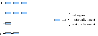
Figure 5: Linked lists of three ungapped alignment fields.

3.3.5 stage 4: Trace-back & display.

In this stage, trace-back information optimizes the alignments recorded in the previous stage and displays them to the user. It is similar to The NCBI BLAST-P processing.

4 PLAST-P sequential version

4.1 Code profiling

The execution time of each stage are detailed in Table 3. In this experiment, data input are bank1 and bank2 (cf. Annex 1). Stage 2 and stage 3.1 respectively consumed an average of 71.8% and 17.5% of the total execution time.

Stage	Task	Percentage of overall time
0	Index the two banks	0.1%
1	Construct neighborhood blocks	0.2%
2	Perform ungapped alignment	71.8%
3-1	Perform small gapped alignment	17.5%
3-2	Perform full gapped alignment	7.9%
4	Trace-Back information and display alignments	2.4%

Table 3: Average runtime for each stage of PLAST-P algorithm when taking as input bank1 and bank2.

The processing times of both ungapped and small gapped alignments represent the majority of the runtime. Thus, to get a significant speed up, both stages need to be optimized. To improve the performances of these stages, two methods have been implemented. The first one is based on the distribution of values in the substitution matrix, and acts as a filter which eliminates hits generating potentially not good alignments. The second approach uses Single-Instruction Multiple Data (SIMD), a technique employed to achieve data level parallelism.

4.2 Filter optimization

The filter aims to eliminate hits providing not a good environment to produce significant ungapped alignments. Its function is based on the distribution of scores which are greater than zero in the substitution matrix (about 15%). A score between two sequences is calculated as the sum of all amino acids pairwise having a matrix score greater than zero. Thus, $|nb1|\times|nb2|$ scores are computed and only pairs of sequences exceeding a threshold values $S_{0}$ are considered as good candidates for the next stage.

To implement this filter, a three-dimensional table stores the positions of scores greater than zero between all amino acids in block nb1. The three dimensions correspond respectively to (1) the number of elements in block nb1, (2) the length of the subsequences and (3) the number of amino-acid (20).

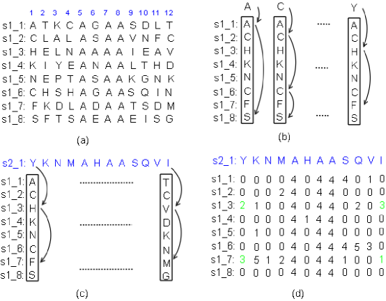
Figure 6: Filtering based on the calculation of a raw score for subsequences of 12 amino-acids.

One example is shown Figure 6: nb1 contains 8 subsequences (s1_1, s1_2, …, s1_8) of length 12. For each character position in the subsequences, 20 linked lists are created (they correspond to the 20 amino acids). Each linked list contents the positions of the amino acid where the score is superior to zero. The next step is to compute the score between subsequence (s2_1) in block nb2 with the 8 subsequences in nb1. To do this, for each amino acid in subsequence s2_1, one linked list corresponding to this acid amino is chosen (Figure 6.c). Based on the elements in this linked list, we calculate a score as depicted Figure 6.d.

To evaluate the filter, the protein bank1 and bank2 (cf. Annex 1) have been considered as input data. Measures indicate that the filter can reduce the execution time of 50% compared to direct ungapped alignment. Only 2,5% of the hits are really processed by the original ungapped procedure. In that scheme, the filtering time represents about 86% of the overall ungapped alignment stage.

Table 4 shows the new code profiling when the filter is activated. It can be seen that the second and third (3-1) stages are still time consuming (82% of the total execution time).

Stage	Task	Percentage of overall time
0	Index the two banks	0.1%
1	Construct neighborhood blocks	0.2%
2	Perform ungapped alignment	55.8%
3-1	Perform small gapped alignment	26.4%
3-2	Perform full gapped alignment	11.8%
4	Trace-Back and display alignments	3.6%

Table 4: Average runtime for each stage of PLAST-P algorithm taking as input bank1 and bank2 with filter optimization.

4.3 SIMD optimization

4.3.1 Ungapped alignments

Generally, the scores of ungapped alignments are small since they are computed on subsequences of limited size. Hence, they need a small number of bits to store the integer values. Here, 1 byte is enough for allowing a 128-bit SIMD register to contain 16 scores.

                 block nb1                                block nb2
    s1_01: .. K C A G A A S D ..             s2_01: .. N M A H A A S Q ..
    s1_02: .. A G A S A A V N ..
    s1_03: .. L N A A A A W E ..

    ...

    s1_14: .. S H A G A A S Q ..
    s1_15: .. W Q A D A A T S ..
    s1_16: .. T S A E A A E M ..

In our implementation, the idea is to compute in parallel the score of 16 subsequences from block nb1 with 1 subsequence of block nb2 as shown on the above figure. If the score exceeds the 8-bit range, it is tagged as an overflow value and passed to next stage.

4.3.2 Gapped alignments

SIMD instructions are also used for speeding up the execution of the small gapped alignment step. To exploit SIMD parallelism, ungapped alignments (coming from the previous step) are first stored in a list. When the list contains at least K elements, they are processed in a SIMD fashion for computing gapped extension.

Unlike ungapped alignments, the score of gapped extensions generally exceed 255 (8-bit). Thus, the SIMD registers use a 16-bit partitioning.

                   bank1                                 bank2
   s1_1: P L..K S A G A A S G..S R       s2_1: R N..A D A H A A G P..K R
   s1_2: I K..R N A S A A F K..Y L       s2_2: F E..Q Q A G A A F K..Y Q
   s1_3: F I..V R A A A A K Q..L I       s2_3: F F..G Q A N A A K I..Q A
   s1_4: D F..I V A N A A Q D..P K       s2_4: D F..Y G A P A A I F..A K
   s1_5: G D..R I A S G A E L..S D       s2_5: L Q..L I A K A A E V..M E
   s1_6: Q G..H R A G A A L S..D I       s2_6: Q L..H L A R A A V N..E K
   s1_7: K S..D L A D A A E I..F S       s2_7: L T..N F A N A A D F..F S
   s1_8: S F..R S A E A A Q N..I L       s2_8: G P..G F A T A A Q N..L L

Here, the SIMD implementation considers the computations of 8 alignments in parallel, each of one performing the Smith-Waterman algorithm restricted to a limited diagonal [21]. The figure above illustrates the data involved in one iteration. The SIMD algorithm can be found in Annex 3.

To evaluate the benefit of the SIMD parallelism, the protein bank1 and bank2 (cf. Annex 1) have been considered as input data. For ungapped (respectively small gapped) alignments, SIMD implementation achieves a speed-up ranging from 4 to 6 (respectively 2.5 to 3) compared to the filter implementation.

Table 5 shows that the second and third (3-1) stages still consumed about 57.5% of the total execution time.

Stage	Task	Percentage of overall time
0	Index the two banks	0.4%
1	Construct neighborhood blocks	0.7%
2	Perform ungapped alignment	33%
3-1	Perform small gapped alignment	24.5%
3-2	Perform full gapped alignment	32.1%
4	Trace-Back and display alignments	9.3%

Table 5: Average runtime for each stage of PLAST-P algorithm taking as input bank1 and bank2 with SIMD 16-bit optimization.

4.4 Perfornamces

In this section, we report measures of the different implementations of PLAST-P. For each of them, the same data set is used: bank1 (141.7K sequences) and bank2 (5K, 10K, 20K, 40K sequences).

4.4.1 Total execution time

Table 6 reports the total execution time of NCBI BLAST-P and four implementations of PLAST-P. The last column is dedicated to the NCBI BLAST-P using default parameters (e-value = 0.001). The second column (PLAST-P – no opt) corresponds to the program PLAST-P with no optimization. The third column (PLAST-P – filter) includes the filter optimization. The two next columns are related to the SIMD implementation, first, with SIMD registers partitioned into 8 16-bit registers (PLAST-P – SIMD 16 bit) and, second, with SIMD registers partitioned into 16 8-bit registers for the ungapped extension stage only.

nb. seq.	PLAST-P	PLAST-P	PLAST-P	PLAST-P	BLAST-P
bank2	(no opt.)	(filter)	(SIMD 16-bit)	(SIMD 8-bit)	(NCBI)
5k	3,766	2,570	940	857	3,521
10k	7,188	4,741	1,775	1,585	6,832
20k	14,394	9,333	3,489	3,188	13,597
40k	28,397	18,996	6,677	6,053	26,111

Table 6: Execution time (sec) of BLAST-P and various versions of PLAST-P.

nb. seq.	PLAST-P	PLAST-P	PLAST-P	PLAST-P
bank2	(no opt.)	(filter)	(SIMD 16-bit)	(SIMD 8-bit)
5k	0.93	1.37	3.74	4.1
10k	0.95	1.44	3.84	4.3
20k	0.94	1.45	3.89	4.26
40k	0.91	1.37	3,91	4.31

Table 7: Speed-up of PLAST-P compared to BLAST-P.

From Tables 6 and 7, it can be seen that the SIMD implementation is much more efficient than the filter optimization. It achieves a global speed up of 4.3 compared to NCBI BLAST-P.

4.4.2 Execution time of ungapped alignments

As the ungapped extension step is very time consuming, it is important to have a closer look on the way the different implementations improve this critical part. Table 8 reports the different execution times. The 8-bit SIMD implementation provides a speed-up of 12 compared to the original code.

nb. seq.	PLAST-P	PLAST-P	PLAST-P	PLAST-P
bank2	(no opt.)	(filter)	(SIMD 16-bit)	(SIMD 8-bit)
5k	2,741	1,511	312	230
10k	5,195	2,643	600	423
20k	10,187	5,102	1,204	830
40k	20,259	10,256	2,237	1,534

Table 8: Execution time (sec) of ungapped alignment in different implementations.

nb. seq.	PLAST-P	PLAST-P	PLAST-P
bank2	(filter)	(SIMD 16-bit)	(SIMD 8-bit)
5k	1.81	8.78	11.91
10k	1.96	8.65	12.28
20k	1.99	8.46	12.27
40k	1.95	9.05	13.02

Table 9: Speed-up of ungapped alignment compared to no optimization.

4.4.3 Selectivity of stage 2

The stage 2 acts as a filter to eliminate hits which have not a good chance to provide significant alignments. Hits are discarded if the score of ungapped alignments are lower than a threshold value. We can then measure the percentage of hits which pass successfully this stage, as it is shown table 10. Lower this percentage, smaller the number of gap extensions to perform. From table 10, it can be seen that the filter optimization loses a few hits compared to other implementations.

nb. seq.	% successful ungapped extension			number of alignments found
bank2	(no opt.)	(filter)	(SIMD)	(no opt.)	(filter)	(SIMD)
5k	0.186%	0.166%	0.186%	305,493	305,044	305,498
10k	0.185%	0.165%	0.185%	611,005	610,543	611,093
20k	0.185%	0.165%	0.185%	1,059,776	1,058,660	1,059,822
40k	0.184%	0.165%	0.184%	2,237,061	2,235,328	2,237,122

Table 10: Results of different PLAST-P sequential implementations.

4.4.4 Sensitivity

Based on the definition of two equivalent alignments (see cf. Annex 2), we compared the sensitivity between PLAST-P and BLAST-P implementations. Here, the 8-bit SIMD optimization is only considered as it provides the best performances. The sensitivity is evaluated by considering three values of % margin: 2% 5% and 10% (cf Annex 2). Table 11 summarizes the results. For each test, the number of alignments found by BLAST-P and SIMD PLAST-P is specified as a percentage of equivalent alignments.

nb. seq	nb. alig. BLAST-P	nb. alig. PLAST-P	2%	5%	10%
5k	305,435	305,489	94.7%	94.9%	95.4%
10k	611,031	611,093	95.3%	95.3%	95.8%
20k	1,047,794	1,059,822	94.8%	95.0%	95.4%
40k	2,237,076	2,237,122	94.5%	95.2%	95.6%

Table 11: Comparison of sensitivity between PLAST-P and BLAST-P

Both programs (BLAST-P and PLAST-P) detect about the same number of alignments, and approximately 95 % of the alignments are equivalent. The difference can be explained as both programs don’t consider the same seeds to detect hits. Thus, there are some alignments found by BLAST-P and not by PLAST-P and, on the contrary, some alignments found by PLAST-P and not by BLAST-P. As an example, Figure 7 presents two alignments which have not been detected by each program. The first alignment is found by PLAST-P and not by BLAST-P because it doesn’t exist a pair of hits on the same diagonal. The second alignment is found by BLAST-P, but not by PLAST-P because the subset seed system of PLAST-P did not detect such hits.

Alignment 1 (found by PLAST-P)

     I980: 112  STKIMKSAIIADSATIGKNCYIGHNVVIEDDVIIGDNSIID----AGTFIGRGVNIGKNA  167
                + KI  SA+I  + TIG N  +G    I+  V++ ++ + D      T +G    IGK A
     P190: 261  TAKIHPSALIGPNVTIGPNVVVGEGARIQRSVLLANSQVKDHAWVKSTIVGWNSRIGKWA  320
     I980: 168  RIEQHVSINYAIIGDD--V---VILVGAK  191
                R E        ++GDD  V   + + GAK
     P190: 321  RTE-----GVTVLGDDVEVKNEIYVNGAK  344

Alignment 2 (found by BLAST-P)

     I914: 109  HSCFNMSSSVMKQMRNQNYGRIVNISSINAQAGQIGQTNYSAAKAGIIGFTKALARETAS  168
                     M  + +  M+ +  GR++   S+    G      Y A+K  + G  ++LA
     1FDV: 116  VGTVRMLQAFLPDMKRRGSGRVLVTGSVGGLMGLPFNDVYCASKFALEGLCESLAVLLLP  175
     I914: 169  KNITVNCIAPGYIATEMVNTV---PKDILTK  196
                  + ++ I  G + T  +  V   P+++L +
     1FDV: 176  FGVHLSLIECGPVHTAFMEKVLGSPEEVLDR  206

Figure 7: Example of two alignments: (1) found by PLAST-P; (2) found by BLAST-P.

5 PLAST-P parallel version

This section presents three parallel version of PLAST-P. The first one – multicore PLAST-P – works on multicore processors, the second one – GPU PLAST-P – uses graphic processors to accelerate stage 2 and stage 3-2 and the final version – multicore GPU PLAST-P – combines the two approaches.

5.1 Multicore processors

On the PLAST-P algorithm, it can be noticed that stages 1, 2 and 3 can be computed independently for each seed. Thus, if M is the number of all the possible seeds, then the PLAST-P algorithm can be splitted into M different processes working separately.

As the number of available CPUs on a multicore processor is much less, one CPU will have – on average – the charge of computing $\frac{M}{P}$ tasks. For load balancing purpose, a CPU is not initialized with a predefined list of tasks. It is just initialized with one task assigned to one specific seed. When its task is finished, it asks for another seed to process. The program stops when there are no more tasks to process.

In summary, the sequential algorithm is changed into a parallel algorithm as follows:

PLAST-P parallel algorithm on multicore processors
Main thread
index1 = make index (bank1)	#stage 0
index2 = make index (bank2)
initialize the shared index variable idx = 1
create P slave threads
wait slave threads to finish and join results
Slave threads
while ( idx $\leq$ M ) do
pthread_mutex_lock()
get a seed from idx
modify idx (idx++)
pthread_mutex_unlock()
construct two neighbouring blocks (nb1 & nb2)	#stage 2
for all hits between nb1 and nb2
compute ungapped alignment
if score $\geq S_{1}$
compute small gapped alignment	#stage 3.1
if score $\geq S_{2}$
compute full gapped alignment	#stage 3.2
if score $\geq S_{3}$
store them in T_ALIGN[$P_{i}$]
end while
trace-back alignments in T_ALIGN[$P_{i}$]	#stage 4

The implementation has been done with the pthread library: the main thread performs sequentially stage 0, then creates P slave threads to perform in parallel stages 1, 2 and 3 for each seeds. Alignments detected by thread $P_{i}$ are stored in its private T_ALIGN structure. When there are no more seed task to process, each threads perform stage 4 for alignments in their T_ALIGN structure.

5.2 GPU - Graphics Processing Units

During the last decade, GPUs [4] have been developed as highly specialized processors for the acceleration of graphical processing. The GPUs have several advantages over CPU architectures for highly parallel intensive workloads, including higher memory bandwidth, significantly higher floating-point capability, and thousands of hardware thread contexts with hundreds of parallel processing units executing programs in a single instruction multiple data (SIMD) fashion.

Recently (2007), NVIDIA has introduced the Geforce 8800 GTX board together with a C-language programming called CUDA [4] (Compute Unified Device Architecture). Geforce 8800 GTX architecture comprises 16 multiprocessors. Each multiprocessor has 8 SPs (Streaming Processors) for a total of 128 SPs. Each group of 8 SPs shares one L1 data cache. A SP contains a scalar ALU (Arithmetic Logic Unit) and can perform floating point operations. Instructions are executed in a SIMD mode.

On the GPU, threads are organized in blocks. A grid of thread blocks is executed on the device. Thread blocks have the same dimensions, and are processed by only one multiprocessor, so that the shared memory space resides in the on-chip shared memory leading to very fast memory accesses. A multiprocessor can process several thread blocks concurrently by partitioning among the set of registers and the shared memory.

For each seed, $|nb1|\times|nb2|$ ungapped alignments are performed in parallel by the GPU. The ungapped extensions passed to the stage 3.1 are stored in a list. When this list contains at least K elements, all elements on this list are considered for small gapped alignment, again on the GPU.

5.2.1 Ungapped alignment

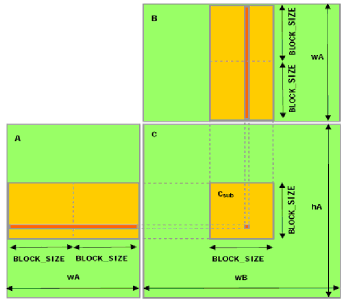
Figure 8: Computing ungapped alignment on GPU.

We implemented the ungapped alignment stage by adapting the matrix multiplication algorithm given in the CUDA documentation [4]. For each seed, there are two subsequence blocks. Suppose that block A[wA, hA] corresponds to block nb1: wA is the length of subsequences, and hA is the number of subsequences in block nb1, and block B[wB, hB] corresponds to block nb2: wB is the number of subsequences in block nb2, and hB is the length of subsequences. Actually, Block B is the transposition of block nb2. Furthermore, we use an other block C[hA, wB] to store scores of ungapped alignments between block nb1 and block nb2. The value of each cell[i,j] in block C corresponds to the score of subsequence j (row j of block nb1) and subsequence i (column i of block nb2).

The task of $|nb1|\times|nb2|$ ungapped alignments between block A and block B is split among threads on GPU as followed: each thread block is responsible for computing a square subblock $C_{sub}$ of C. Each thread within the block is responsible for computing one element of $C_{sub}$ (Figure 8). The dimension block_size of $C_{sub}$ is chosen to be equal to 16. Thus, there are $\frac{hA}{16}$ x $\frac{wB}{16}$ thread blocks in grid. Threads within the same block share the same memory space.

Two subsequence blocks are mapped to the texture memory of the GPU. The texture memory is shared by all the processors, and speed up comes from its space which is implemented as a read-only region of the device memory. At the beginning of the computation, each thread loads a character from the texture memory to the shared memory using a texture reference, called texture fetching.

5.2.2 Small gapped alignments

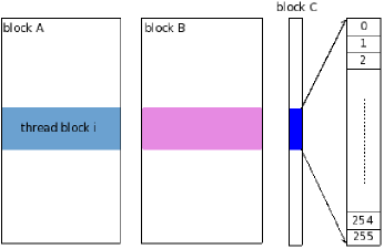
Figure 9: Computing small gapped alignment on GPU.

The use of high performance computing on GPU is efficient only to perform large tasks. Thus, we use the GPU to execute small gapped alignments when there are at least K elements ready for computation. With K small gapped alignments, there are K extensions - extending in two directions. To be able to compute 2K extensions on the GPU, we have to construct two subsequence blocks as already done for ungapped alignment: one block (A) for bank1 and one block (B) for bank2. Compared to ungapped alignment, there is a difference: for one small gapped alignment, we copy two subsequences in bank1 - one at the left and one at the right of the seed - to block A, and two subsequences (bank2) to block B. Consequently, there are 2K subsequences in each block. The GPU divides 2K extensions into thread blocks; each thread within a block is responsible for computing one extension.

The form of thread block is $1\times 256$. Thus, there are $\frac{2K}{256}$ thread blocks. Two subsequence blocks are mapped to the texture memory. At the beginning of the computation, each thread copies its pair of subsequences from the texture memory by the texture reference to its local memory for reducing memory access conflict. The scores of 2K extensions are stored in block C[2K,1] as shown Figure 9.

5.3 Multicore processors and GPU

This section describes a parallelization based on a platform made of a single dual core processor and a single GPU board. The parallelization works as follows: the first core constructs the two neighborhood blocks and controls the computation – ungapped alignment and small gapped alignment – on the GPU. The second core performs full gapped alignment and stage 4. The two cores communicate together by a queue Q. The multicore GPU parallel algorithm can be described as follows:

Multicore GPU PLAST-P algorithm
	index1 = make index (bank1)	#stage 0
	index2 = make index (bank2)
Processor 1
	for all possible seeds
	construct neighborhood block nb1 from index1	#stage 1
	construct neighborhood block nb2 from index2
	compute $|nb1|\times|nb2|$ ungapped alignments on GPU	#stage 2
	store ungapped alignments if score $\geq S_{1}$ in list R
	if the list R contains at least K elements
	compute K small gapped alignments on GPU	#stage 3.1
	store small gapped alignments if score $\geq S_{2}$ in queue Q
	deleted K elements in R
	flag = FALSE
Processor 2
	while(flag==TRUE)
	if list Q != $\varnothing$
	compute full gapped alignment for all elements in Q	#stage 3-2
	if score $\geq S_{3}$
	trace-back display alignment	#stage 4

5.4 Perfornamces

In this section, we report measures of the different parallel implementations of PLAST-P. For each of them, the same data set is used: bank1 and bank2(cf. Annex 1).

The multicore processors version has been tested with the SIMD 8-bit optimization. The GPU version uses the NVIDIA GeForce 8800 graphic board (cf. Annex 1). The multicore-GPU version combines the two approaches: dual core processor + GPU board.

5.4.1 Total execution time

The execution time is compared between the different parallel versions of PLAST-P and the parallel version of the NCBI BLAST-P program. Actually, BLAST-P can be run on a parallel machine by specifying the number of nodes. For this experimentation, this option (- a) has been set to 2.

nb. seq.	multi	GPU	multi-GPU	multicore
bank2	PLAST-P	PLAST-P	PLAST-P	BLAST-P
5k	472	646	379	1,953
10k	889	1,186	692	3,794
20k	1,761	2,420	1,442	7,573
40k	3,282	4,581	2,745	14,281

Table 12: Execution time (sec) of multicore BLAST-P and various versions of PLAST-P.

nb. seq.	multi	GPU	multi-GPU
bank2	PLAST-P	PLAST-P	PLAST-P
5k	4.13	3.02	5.15
10k	4.26	3.19	5.48
20k	4.30	3.12	5.25
40k	4.35	3.11	5.20

Table 13: Speed-up of PLAST-P compared to multicore BLAST-P

Table 12 reports the total execution time for various size of bank2. Both the execution times of multicore BLAST-P and multicore PLAST-P are reduced by about 55% when compared to their sequential version (Table 6). Similarly, the multicore PLAST-P program achieves an acceleration factor of 4.2 compared to the multicore BLAST-P program.

When comparing performances between multicore PLAST-P and GPU PLAST-P, multicore PLAST-P gains 25% over the GPU PLAST-P program. This can be explained as follows: The execution time of stage 3-1 and stage 4 in GPU PLAST-P represents 63% of the total execution time and only stage 2 and 3-1 are performed in parallel. In the multicore GPU PLAST-P version, the first processor and GPU take about 40% of the execution time. The second takes about 60%, so that this version obtained a 40% speed-up over the GPU version.

5.4.2 Selectivity of stage 2

We have examined the number of alignments found in different PLAST-P parallel implementations. The percentage of ungapped alignments considered as successful is presented in Table 14. The percentage of successful ungapped alignments in multicore PLAST-P is the same as in the sequential version (with SIMD optimization). Thus, the number of alignments found by both versions is also equal.

However, the percentage of successful ungapped alignments in the two GPU versions is higher than the others because of the computation performed on the GPU: the length of the subsequences (in the ungapped extension stage) must be a multiple of 16. Thus, subsequences are longer than the subsequences of other versions. Consequently, the percentage of successful ungapped alignments increases.

nb. seq.	% successful ungapped extension			number of alignments found
bank2	multi	GPU	multi-GPU	multi	GPU	multi-GPU
5k	0.186%	0.194%	0.194%	305,502	305,663	305,662
10k	0.185%	0.193%	0.193%	611,154	610,993	610,989
20k	0.185%	0.193%	0.193%	1,059,796	1,062,130	1,062,129
40k	0.185%	0.192%	0.193%	2,237,086	2,237,140	2,237,137

Table 14: Results of different PLAST-P parallel implementations.

5.4.3 GPU Execution time

The computing times of ungapped and small gapped alignments are reported in Table 15. The second column shows execution time of ungapped alignment in PLAST-P program (sequential version with filter optimization). In GPU PLAST-P program, GPU achieved a speed-up ranging from 8.5 to 10. The execution times of small gapped alignments are presented in the three last columns. As it can be seen, GPU also achieved a speed-up ranging from 9 to 11 for when comparing with the version without optimization.

nb. seq.	ungapped extension		small gapped extension
bank2	filter opt.	GPU	no opt.	SIMD 8-bit	GPU
5k	1,511	148 (10.21)	626	226 (2.76)	64 (9.78)
10k	2,643	295 (8.95)	1,232	443 (2.78)	136 (9.05)
20k	5,102	594 (8.59)	2,602	822 (3.16)	275 (9.64)
40k	10,256	1,079 (9.51)	5,213	1,564 (3.33)	470 (11.09)

Table 15: Execution time (sec) of ungapped and small gapped alignment in different implementations. Numbers in brackets represent speed-up.

6 TPLAST-N

A TBLAST-N search compares a protein sequence to the six translated frames of a nucleotide database. It can be a very productive way of finding homologous proteins in an unannotated nucleotide sequence. Like BLAST-P, TBLAST-N is not specifically adapted for intensive sequence comparison. Thus, similarly to PLAST-P, TPLAST-N uses the double indexing technique for speeding up the search. In this section, details of implementation are not described. We only focus on the TPLAST-N program performances.

All the measures have been done with the following data set:

• DNA bank: bank3 (cf. Annex 1)

• 4 protein banks: bank2 (cf. Annex 1)

6.1 TPLAST-N sequential version

This section presents the performances of three sequential versions:

• no optimization: TPLAST-N (no opt.)

• filter optimization: TPLAST-N (filter)

• SIMD optimisation: TPLAST-N (SIMD)

6.1.1 TPLAST-N Profiling

Table 16 shows the percentage of time spent in the different stages of the TPLAST-N (no opt.) program. Again, stages 2 and 3.1 are good candidates for parallelization since 72% and 23% of the execution time is spent in these two stages.

Stage	Task	Percentage of overall time
0	Index the two banks	0.4%
1	Construct neighborhood blocks	0.6%
2	Perform ungapped alignment	72.0%
3-1	Perform small gapped alignment	23.0%
3-2	Perform full gapped alignment	2.7%
4	Trace-Back information and display alignments	1.3%

Table 16: Average runtime for each stage of TPLAST-N (no opt.)

6.1.2 Execution time

Table 17 shows the total execution time (in second). Note that TPLAST-N (no opt.) is slower than TBLAST-N (about 10 % slower).

nb. seq.	TPLAST-N	TPLAST-N	TPLAST-N	TPLAST-N	TBLAST-N
bank2	(no opt.)	(filter)	(SIMD 16-bit)	(SIMD 8-bit)
5k	7,817	5,392	1,491	1,328	7,036
10k	15,261	9,704	2,789	2,394	13,784
20k	30,332	18,069	5,411	4,554	27,147
40k	57,987	33,540	10,232	8,553	52,232

Table 17: Execution time (sec) of TBLAST-N and the three sequential implementations of TPLAST-N.

nb. seq.	TPLAST-N	TPLAST-N	TPLAST-N	TPLAST-N
bank2	(no opt.)	(filter)	(SIMD 16-bit)	(SIMD 8-bit)
5k	0.90	1.30	4.71	5.29
10k	0.90	1.42	4.94	5.75
20k	0.89	1.50	4.98	5.96
40k	0.90	1.55	5.10	6.10

Table 18: Speed-up of TPLAST-N compared to TBLAST-N.

Table 18 shows that the 8-bit SIMD implementation provides the best performances with a speed-up ranging from 5 to 6 compared to the NCBI TBLAST-N implementation.

Table 19 shows the execution time (in second) of the ungapped alignment stage only (stage 2).

nb. seq.	TPLAST-N	TPLAST-N	TPLAST-N	TPLAST-N
bank2	(no opt.)	(filter)	(SIMD 16-bit)	(SIMD 8-bit)
5k	6,495	4,333	832	681
10k	12,590	7,264	1,549	1,165
20k	25,385	13,325	3,032	2,173
40k	48,408	24,251	5,682	3,963

Table 19: Execution time (sec) of ungapped alignment in different implementations.

nb. seq.	TPLAST-N	TPLAST-N	TPLAST-N
bank2	(filter)	(SIMD 16-bit)	(SIMD 8-bit)
5k	1.49	7.80	9.53
10k	1.73	8.12	10.80
20k	1.90	8.37	11.68
40k	1.99	8.50	12.21

Table 20: Speed-up of ungapped alignment compared to no optimization.

6.1.3 Selectivity of stage 2

Table 21 gives the percentage of hits which have produced successful ungapped alignments (stage 2) and the total number of alignments generated by the TPLAST-N programs.

nb. seq.	% successful ungapped extension			number of alignments found
bank2	(no opt.)	(filter)	(SIMD)	(no opt.)	(filter)	(SIMD)
5k	0.145%	0.127%	0.146%	290,378	290,277	290,387
10k	0.148%	0.129%	0.149%	573,238	572,057	573,248
20k	0.145%	0.127%	0.145%	1,173,396	1,166,243	1,172,422
40k	0.147%	0.128%	0.147%	2,211,782	2,198,534	2,211,808

Table 21: Selectivity of stage 2 and number of alignments found by the TPLAST-N sequential implementations.

6.1.4 Sensibility

The table 22 compares the sensitivity of TBLAST-N and TPLAST-N (SIMD) following the criteria described in Annex 2.

nb. seq	nb. alig. TBLAST-N	nb. alig. TPLAST-N	2%	5%	10%
5k	290,016	290,387	95.6%	95.7%	95.9%
10k	572,608	573,248	96.0%	96.2%	96.4%
20k	1,172,466	1,172,422	96.4%	96.5%	96.6%
40k	2,208,330	2,211,808	96.4%	96.6%	96.7%

Table 22: Comparison of sensitivity between TPLAST-N and TBLAST-N

6.2 TPLAST-N parallel version

This section presents the performances of three parallel versions of TPLAST-N:

• multicore: TPLAST-N (multi)

• grapics board: TPLAST-N (GPU)

• multicore + graphics board: TPLAST-N (multi-GPU)

6.2.1 Execution time

Table 23 compares the total execution time of the parallel TPLAST-N programs and the NCBI TBLAST-N program run with the -a option.

nb. seq.	multi	GPU	multi-GPU	multicore
bank2	TPLAST-N	TPLAST-N	TPLAST-N	TBLAST-N
5k	746	773	617	3,859
10k	1,341	1,372	1,096	7,509
20k	2,503	2,613	2,064	14,831
40k	4,741	4,942	4,016	28,674

Table 23: Execution time (sec) of multicore TBLAST-N and the three parallel implementations of TPLAST-N

nb. seq.	multi	GPU	multi-GPU
bank2	TPLAST-N	TPLAST-N	TPLAST-N
5k	5.17	4.99	6.25
10k	5.59	5.47	6.85
20k	5.92	5.67	7.18
40k	6.04	5.80	7.13

Table 24: Speed-up of TPLAST-N compared to multicore TBLAST-N

The best performances are provided by the TPLAST-N (multi-GPU) program with a speed-up ranging from 6 to 7 compared to the NCBI TBLAST-N program as showed in Table 24.

Table 25 indicates the sequential and parallel execution times of stage 2 (ungapped alignments) and stage 3.1 (small gapped alignments).

nb. seq.	ungapped extension		small gapped extension
bank2	filter	GPU	no opt.	SIMD 8-bit	GPU
5k	4,333	378 (11.46)	1,050	436 (2.40)	120 (8.75)
10k	7,264	703 (10.33)	2,103	872 (2.41)	259 (8.11)
20k	13,325	1,361 (9.79)	4,088	1,686 (2.42)	462 (8.48)
40k	24,251	2,589 (9.36)	7,866	3,233 (2.43)	893 (8.80)

Table 25: Execution time (sec) of ungapped and small gapped alignment in different implementations. Numbers in brackets represent speed-up.

6.2.2 Selectivity of stage 2

Table 26 gives the percentage of hits which have produced successful ungapped alignments (stage 2) and the total number of alignments generated by the parallel versions of TPLAST-N.

nb. seq.	% successful ungapped extension			number of alignment found
bank2	multi	GPU	multi-GPU	multi	GPU	multi-GPU
5k	0.146%	0.154%	0.154%	290,378	290,406	290,403
10k	0.149%	0.158%	0.158%	573,252	573,880	573,881
20k	0.145%	0.153%	0.153%	1,172,415	1,173,378	1,173,378
40k	0.147%	0.156%	0.156%	2,211,867	2,211,935	2,211,953

Table 26: Selectivity of stage 2 and number of alignments found by the TPLAST-N parallel implementations.

7 PLAST-X

BLAST-X compares translational products of the nucleotide query sequence to a protein database. BLAST-X is often the first analysis performed with a newly determined nucleotide sequence. Like BLAST-P and TBLAST-N, BLAST-X is not specifically adapted for intensive sequence comparison. Thus, similarity to PLAST-P, PLAST-X uses the double indexing technique for speeding up the search. In this section, details of implementation are not described. We only focus on the PLAST-X program performances.

All the measures have been done with the following data set:

• DNA bank: bank3 (cf. Annex 1)

• 4 DNA banks: bank4 (cf. Annex 1)

7.1 PLAST-X sequential version

This section presents the performances of three sequential versions:

• no optimization: PLAST-X (no opt.)

• filter optimization: PLAST-X (filter)

• SIMD optimisation: PLAST-X (SIMD)

7.1.1 PLAST-X Profiling

Table 27 shows the percentage of time spent in the different stages of the PLAST-X (no opt.) program. Again, stages 2 and 3.1 are good candidates for parallelization since 79% and 13.8% of the execution time is spent in these two stages.

Stage	Task	Percentage of overall time
0	Index the two banks	0.4%
1	Construct neighborhood blocks	0.5%
2	Perform ungapped alignment	79.0%
3-1	Perform small gapped alignment	13.8%
3-2	Perform full gapped alignment	5.3%
4	Trace-Back information and display alignments	1.0%

Table 27: Average runtime for each stage of PLAST-X (no opt.)

7.1.2 Execution time

Table 28 shows the total execution time (in second). Note that PLAST-X (no opt.) is slower than BLAST-X (about 20 % slower).

nb. seq.	PLAST-X	PLAST-X	PLAST-X	PLAST-X	BLAST-X
bank4	(no opt.)	(filter)	(SIMD 16-bit)	( SIMD 8-bit)
1k	1,775	1,210	369	328	1,501
3k	5,583	3,345	1,186	1,028	4,455
6k	10,737	6,262	2,302	1,989	8,495
10k	18,125	10,588	4,089	3,523	14,035

Table 28: Performance between PLAST-X and BLAST-X.

nb. seq.	PLAST-X	PLAST-X	PLAST-X	PLAST-X
bank2	(no opt.)	(filter)	(SIMD 16-bit)	(SIMD 8-bit)
1k	0.84	1.24	4.06	4.57
3k	0.79	1.33	3.76	4.33
6k	0.79	1.35	3.69	4.27
10k	0.77	1.32	3.43	3.98

Table 29: Speed-up of PLAST-X compared to BLAST-X.

The 8-bit SIMD implementation provides the best performances with a speed-up ranging from 4 to 4.5 compared to the NCBI BLAST-X implementation.

Table 30 shows the execution time (in second) of the ungapped alignment stage only (stage 2).

nb. seq.	PLAST-X	PLAST-X	PLAST-X	PLAST-X
bank4	(no opt.)	(filter)	(SIMD 16-bit)	(SIMD 8-bit)
1k	1,449	918	182	143
3k	4,424	2,338	530	378
6k	8,439	4,312	1,004	700
10k	13,941	6,994	1,680	1,156

Table 30: Execution time (sec) of ungapped alignment in different implementations.

nb. seq.	PLAST-X	PLAST-X	PLAST-X
bank2	(filter)	(SIMD 16-bit)	(SIMD 8-bit)
1k	1.57	7.96	10.13
3k	1.89	8.34	11.70
6k	1.95	8.40	12.05
10k	1.99	8.29	12.05

Table 31: Speed-up of ungapped alignment compared to no optimization.

7.1.3 Selectivity of stage 2

Table 32 gives the percentage of hits which have produced successful ungapped alignments (stage 2) and the total number of alignments generated by the PLAST-X programs.

nb. seq.	% successful ungapped extension			number of alignments found
bank4	(no opt.)	(filter)	(SIMD)	(no opt.)	(filter)	(SIMD)
1k	0.150%	0.132%	0.150%	32,326	32,310	32,328
3k	0.152%	0.134%	0.152%	97,059	97,010	97,059
6k	0.154%	0.135%	0.154%	196,245	196,168	196,252
10k	0.159%	0.140%	0.159%	332,124	331,928	332,135

Table 32: Selectivity of stage 2 and number of alignments found by the PLAST-X sequential implementations.

7.1.4 Sensibility

The table 33 compares the sensitivity of BLAST-X and PLAST-X (SIMD) following the criteria of the Annex 2.

nb. seq	nb. alig. BLAST-X	nb. alig. PLAST-X	2%	5%	10%
1k	31,873	32,328	94.4%	97.8%	98.3%
3k	94,221	97,059	94.7%	97.9%	98.3%
6k	189,488	196,252	94.6%	98.0%	98.5%
10k	321,416	332,135	94.6%	98.0%	98.5%

Table 33: Comparison of sensitivity between PLAST-X and BLAST-X

7.2 PLAST-X parallel version

This section presents the performances of three parallel versions of PLAST-X:

• multicore: PLAST-X (multi)

• grapics board: PLAST-X (GPU)

• multicore + graphics board: PLAST-X (multi-GPU)

7.2.1 Execution time

Table 34 compares the total execution time of the parallel PLAST-X programs and the NCBI BLAST-X program run with the -a option.

nb. seq.	multi	GPU	multi-GPU	multicore
bank4	PLAST-X	PLAST-X	PLAST-X	BLAST-X
1k	178	191	129	833
3k	564	662	379	2,403
6k	1,093	1,309	778	4,622
10k	1,937	2,462	1,531	7,550

Table 34: Execution time (sec) of multicore BLAST-X and the three parallel implementations of PLAST-X.

nb. seq.	multi	GPU	multi-GPU
bank2	PLAST-X	PLAST-X	PLAST-X
1k	4.60	4.36	6.45
3k	4.26	3.62	6.34
6k	4.22	3.53	5.94
10k	3.89	3.06	4.93

Table 35: Speed-up of PLAST-X compared to multicore BLAST-X

The best performances are provided by the PLAST-X (multi-GPU) program with a speed-up ranging from 5 to 6 compared to the NCBI BLAST-X program.

Table 36 indicates the sequential and parallel execution times of stage 2 (ungapped alignments) and stage 3.1 (small gapped alignments).

nb. seq.	ungapped extension		small gapped extension
bank4	filter opt.	GPU	no opt.	SIMD 8-bit	GPU
1k	918	81 (11.33)	241	101 (2.38)	30 (8.03)
3k	2,338	246 (9.50)	762	319 (2.38)	94 (8.10)
6k	4,312	474 (9.09)	1478	612 (2.41)	166 (8.90)
10k	6,998	854 (8.19)	2568	1,064 (2.41)	316 (8.12)

Table 36: Execution time (sec) of ungapped and small gapped alignment in different implementations. Numbers in brackets represent speed-up.

7.2.2 Selectivity of stage 2

Table 37 gives the percentage of hits which have produced successful ungapped alignments (stage 2) and the total number of alignments generated by the parallel versions of PLAST-X.

nb. seq.	% successful ungapped extension			number of alignments found
bank4	multi	GPU	multi-GPU	multi	GPU	multi-GPU
1k	0.150%	0.158%	0.158%	32,330	32,344	32,344
3k	0.153%	0.161%	0.161%	97,059	97,173	97,173
6k	0.154%	0.162%	0.162%	196,256	196,514	196,514
10k	0.160%	0.168%	0.168%	332,133	332,418	332,418

Table 37: Selectivity of stage 2 and number of alignments found by the PLAST-X parallel implementations

8 Comparison with the BLAST-P family

This section summarizes the performances of the various PLAST-P implementations by comparing the speed-up between the PLAST-P and BLAST-P families.

8.1 BLAST-P vs PLAST-P

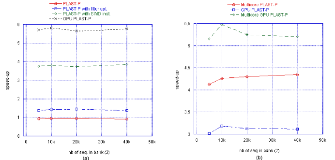
Figure 10: Speed-up of different PLAST-P: (a) over BLAST-P; (b) over multicore BLAST-P.

8.2 TBLAST-N vs TPLAST-N

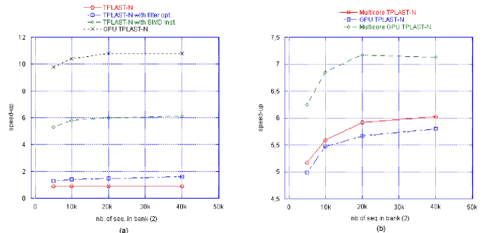
Figure 11: Speed-up of different TPLAST-N: (a) over TBLAST-N; (b) over multicore TBLAST-N.

8.3 BLAST-X vs PLAST-X

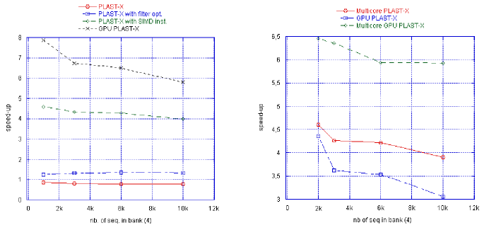
Figure 12: Speed-up of different PLAST-X: (a) over BLAST-X; (b) over multicore BLAST-X.

Annex 1: Hardware and Data Set

Hardware Platform

Processor

We tested the experiments on: An Intel core 2 Dual 2.6 GH processor with 2 MB L2 cache, and 2 GB RAM, running Linux (fedora 6).

Graphic board

We used the graphic card GeForce 8800 GTX (version GPU). The characteristics of this board are the following:

• 16 multiprocessors SIMD at 675 MHz; each multiprocessor is composed of eight processors running at twice the clock frequencies;

• the maximum number of threads per block is 512;

• the amount of device memory is 768 MB at 1.8 GHz engine clock speed;

• the maximum bandwidth observed between the computer memory and the device memory is 2 GB/s.

Data set

• bank1: It contents 141,708 sequences from the PIR-Protein bank (version 80 01/2005) with an average length of 340;

• bank2: Actually, this is a set of four banks extracted from the SWISS-PROT bank (version 05/2007) which content respectively 5,000; 10,000; 20,000, and 40,000 sequences with an average length of 367;

• bank3: It contents 27,360 sequences (gbvrt3 in GenBank, version 156) with an average length of 5,454;

• bank4: This is a set of four banks extracted from the gbvrl division of Genbank (version 156) which content respectively 1,000; 3,000; 6,000, and 10,000 sequences with an average length of 1,024.

Annex 2: Measure criteria

Execution time

The execution time is calculated using the Linux time command. For each experiment, the machine is only dedicated to the computation under test. BLAST was launched with the default settings, except for the e-value statistical parameter set to $10^{-3}$. It represents a reasonable value in the context of intensive sequence comparison.

Sensibility

The sensitivity is evaluated in relation to the number of alignments found in both cases. Specifically, we look at whether alignments found begin and end at the same places in the two sequences with a margin of Y % calculated on the average size of the 2 alignments. For example, to compare two alignments of size 100 with 5% margin, we check that the start and end positions for making up this alignment are within a range of 5 amino acids.

Annex 3: Source codes of SIMD ungapped alignment

    VectUngappedExtend(char **block1, char **block2,
                                   int n1, int n2, HIT *listeRS){

       // n1, n2: number of subsequences in block1 and block2
       short *databk;
       short *pc;
       short score_arr[];
       __m128iΨ*pvb, pvScore, vscore, vMaxScore;
       // declaration of the sequence profile memoryΨΨ
   Ψ   databk = (short *) calloc(SIZE_MT*LenSubSeq, sizeof(__m128i));
       pvb = (__m128i *) databk;
       for(j=0;j<n1;j+=SIZEV){ // SIZEV: number of elements in vector
         pc = (short *) pvb;
         // initiation profile for SIZEV subsequences
         for(i=0;i<SIZE_MT;i++){ // SIZE_MT: size of substitution matrix
            matrixRow = MATRIX[i];  // MATRIX: substitution matrix
            for(k=0;k<LenSubSeq;k++){
               for(l=0;l<SIZEV;l++){
                  *pc++ = (short) matrixRow[block1[j+l][k]];
               }
            }
         }
         // compute scores between SIZEV subsequences in bloc1
         // and all sequences in block2
         for(i=0;i<n2;i++){
            vMaxScore = _mm_xor_si128 (vMaxScore, vMaxScore);
            vscore = _mm_xor_si128 (vscore, vscore);
            for(k=0;k<LenSubSeq;k++){
               pvScore = *(pvb + (block2[i][k] * LenSubSeq + k));
               vscore = _mm_adds_epi16 (vscore, pvScore);
               vMaxScore = _mm_max_epi16 (vMaxScore, vscore);
            }
            // extraction element score
            for(i=0;i<SIZEV;i++)
               score_arr[i] =  _mm_extract_epi16(vMaxScore,i);
            for(k=0;k<SIZEV;k++)
              if(score_arr[k]>=S2) add(ungapped, listRS);
          }
       }
    }

Annex 4: Source gode of GPU ungapped alignment

   GPUngappedExtend(char* h_A, char* h_B, char* h_C, int nba, int nbb){
      // nba, nbb: number of subsequences in block A and block B
      // allocate device memory
      unsigned char* d_A;
      CUDA_SAFE_CALL(cudaMalloc((void**) &d_A, mem_size_A));
      unsigned char* d_B;
      CUDA_SAFE_CALL(cudaMalloc((void**) &d_B, mem_size_B));

      // copy host memory to device
      CUDA_SAFE_CALL(cudaMemcpy(d_A, h_A, mem_size_A,
                              cudaMemcpyHostToDevice) );
      CUDA_SAFE_CALL(cudaMemcpy(d_B, h_B, mem_size_B,
                              cudaMemcpyHostToDevice) );

      // allocate device memory for result
      unsigned int mem_size_C = sizeof(char) * nba * nbb;
      char* d_C;
      CUDA_SAFE_CALL(cudaMalloc((void**) &d_C, mem_size_C));

      // setup execution parameters for block grid
      dim3 threads(BLOCK_SIZE, BLOCK_SIZE);
      dim3 grid(nbb / threads.x, nba / threads.y);

      // execute the kernel
      GPUnGapped_kernel<<< grid, threads >>>(d_C, d_A, d_B, nba, nbb);

      // copy result from device to host
      CUDA_SAFE_CALL(cudaMemcpy(h_C, d_C, mem_size_C,
                              cudaMemcpyDeviceToHost));
   }

   GPUngapped_kernel(char* d_C, char* d_A, char* d_B, int nba, int nbb){

      // block index
      int bx = blockIdx.x;
      int by = blockIdx.y;
      // thread index
      int tx = threadIdx.x;
      int ty = threadIdx.y;
      // index at the beginning of h_A
      int aBegin = nba * BLOCK_SIZE * by;
      aBegin += nba * ty + tx;
      // step size used to iterate through the sub-bloc of A
      int aStep  = BLOCK_SIZE;
      // index at the beginning of h_B
      int bBegin = __mul24(BLOCK_SIZE,bx);
      bBegin += nbb * ty + tx;
      // step size used to iterate through the sub-tabe of h_B
      int bStep  = __mul24(BLOCK_SIZE,nbb);
      // Csub is used to store the elements of the block sub-score
      //that is computed by the thread
      int Csub = 0;
      int CsubMaxi = 0;
      // declaration of the shared memory array As used to
      // store the sub-block of h_A
      __shared__ int As[BLOCK_SIZE][2*BLOCK_SIZE];
      // declaration of the shared memory array Bs used to
      // store the sub-table of h_B
      __shared__ int Bs[2*BLOCK_SIZE][BLOCK_SIZE];
      // load the matrices from device memory to shared memory;
      AS(ty, tx) = A[aBegin];
      BS(ty, tx) = B[bBegin];
      AS(ty, tx + aStep) = A[aBegin + aStep];
      BS(ty + aStep, tx) = B[bBegin + bStep];
      // synchronize to make sure the sub-blocks are loaded
      __syncthreads();
      // calculate the score two sub_blocks together;
      for (int k = 0; k < 2*BLOCK_SIZE; k++){
        Csub = Csub + texfetch(matrix, AS(ty, k), BS(k, tx));
        if(Csub>CsubMaxi) CsubMaxi = Csub;
        if(k==MAX_RIGHT) Csub = CsubMaxi;
      }
      __syncthreads();
      AS(ty, tx) = A[aBegin + 2*aStep];
      BS(ty, tx) = B[bBegin + 2*bStep];
      // synchronize to make sure the sub-blocks are loaded
      __syncthreads();
      for (int k = 0; k < BLOCK_SIZE; k++){
        Csub = Csub + texfetch(matrix, AS(ty, k), BS(k, tx));
        if(Csub>CsubMaxi) CsubMaxi = Csub;
      }
      // write the block sub-matrix to device memory,
      // each thread writes one element
      int c = bStep * by + bBegin;
      C[c] = CsubMaxi;
}

References

- [1] Benson, D., Karsch-Mizrachi, I., Lipman, D., Ostell, J., Wheeler, D., GenBank, Nucleic Acids Research, Vol. 35, pp. 21-25, 2007.
- [2] Ricardo Asencio, Implementation de BLAST sur les cartes graphiques, rapport Master2, 2007.
- [3] Peterlongo, P., Noe, L., Lavenier, D., Georges, G., Jacques, J., Kucherov, G., Giraud, M., Protein similarity search with subset seeds on a dedicated reconfigurable hardware, Parallel Bio-Computing, Gdansk, Poland, 2007.
- [4] NVIDIA CUDA Compute Unified Device Architecture, Programming Guide, version 1.0, 23/6/2007.
- [5] Lavenier, D., Xinchun, L., Georges, G., Seed-based genomic sequence comparison using a FPGA / FLASH accelerator, International IEEE Conference on Field Programmable Technology (FPT), Bangkok, Thailand, 2006.
- [6] Liu, W., Schmidt, B., Voss, G., Schroder, A.& Wolfgang, M., Bio-sequence database scanning on a GPU, HICOMBO, Rhodes Island, Greece, 2006.
- [7] Cameron, M., Williams, H. E. & Cannane, A., A deterministic finite automaton for faster protein hit detection in BLAST, Journal of Computational Biology, Vol 13(4), pp. 965-978, 2006.
- [8] Kucherov, G., Noe, L. & Roytberg, M. A unifying framework for seed sensitivity and its application to subset seeds, JBCB 2006.
- [9] Noe, L. & Kucherov YASS, G. Enhancing the sensitivity of DNA similarity search, NAR 2005.
- [10] Daniel G. Brown, Optimizing multiple seeds for protein homology search, IEEE/ACM Transactions on Computational biology and bioinformatics, Vol. 2, pp. 29-38, 2005.
- [11] Cameron, M., Williams, H. E. & Cannane, A., Improved gapped alignment in BLAST, IEEE Transactions on Computational Biology and Bioinformatics, Vol. 1, No. 3, 2004.
- [12] Li, M., Ma, B., Kisman, D. & Tromp, J., PatternHunter II: Highly sensitive and fast homology search, Journal of Bioinformatics and Computational Biology, Vol 2(3), pp. 417-439, 2004.
- [13] Darling, EA., Carey, L., Feng, W., The design, implementation, and evaluation of mpiBLAST, 4th International Conference on Linux Clusters, San Jose, USA, 2003.
- [14] Williams, H. E. & Zobel, J., Indexing and retrieval for genomic databases, IEEE Transactions on Knowledge and Data Engineering, Vol. 14, pp. 63-78, 2002.
- [15] Ma, B., Tromp, J. & Li, M., PatternHunter: faster and more sensitive homology search, Bioinformatics, Vol 18(3), pp. 440-445, 2002.
- [16] Kent, W., BLAT: the BLAST-like alignment tool. Genome Research, Vol. 12, pp. 656-664, 2002.
- [17] Zhang, Z., Schaer, A., Miller, W., Madden, T., Lipman, D., Koonin, E., and Altschul, S., Protein sequence similarity searches using patterns as seeds, Nucleic Acids Research, Vol. 26, pp. 3986-9390, 1998.
- [18] Altschul, S., Madden, T., Schaffer, A., Zhang, J., Zhang, Z., Miller, W., Lipman, D., Gapped BLAST and PSI-BLAST : A new generation of protein database search programs, Nucleic Acids Research, Vol. 25, No. 17, pp. 3389-3402, 1997.
- [19] Altschul, S., Gish W., Miller W., Myers E. W. & Lipman D., Basic Local Alignment Search Tool, J. Mol. Biology, 215, pp. 403-410, 1990.
- [20] Wilbur, W. and Lipman, D., Rapid similarity searches of nucleic acid and protein data banks. Proceedings of the National Academy of Sciences USA, Vol. 80(3), pp. 726-730 1983.
- [21] Smith, T.F., Waterman, M.S., Identification of common molecular subsequences, J Mol Biol 1981, 147(1), pp. 195-197.
- [22] Genome online database - http://www.genomesonline.org/