Reexamination for the calculation of elliptic flow and other fourier harmonics

Abstract

We have argued that the azimuthal symmetry and asymmetry components in fourier expansion of particle momentum azimuthal distribution, $v_{n}$ (n=0, 1, 2, …), should be calculated as an average of $cos(n\phi)$ first over particles in an event and then over events (event-wise average) rather than “an average over all particles in all events” (particle-wise average). In case of large centrality (multiplicity) bin the particle-wise average is not accurate because the influence (fluctuation) of particle multiplicity was not taken into account.
PACS numbers: 25.75.Dw, 24.85.+p

Elliptic flow (proportional to $v_{2}$) and other harmonics (proportional to $v_{n}$, $n$=0, 1, 3, 4, …) as fourier expansion coefficients of azimuthal distribution of particle momentum are highly sensitive to the eccentricity of the early created fireball in ultra-relativistic heavy ion collisions. The expected phase transition to Quark-Gluon-Plasma (QGP) should have a dramatic effect on those harmonics. The consistency between experimental data of $v_{2}(p_{T})$ at mid-rapidity and the corresponding hydrodynamic predictions are regarded as an evidence of the production of partonic matter in ultra-relativistic nucleus-nucleus collisions miclo . The elliptic flow of high $p_{T}$ particles may be related to the jet fragmentation and parton energy loss wang1 , which are usually not included in the hydrodynamic calculations. This hydrodynamic model kolb overestimates $v_{2}(p_{T})$ in the $p_{T}\geq 1.5$ GeV/c region phob1 . That is regarded, together with the discovery of jet quenching zajc , as a strong evidence of sQGP formation in relativistic nucleus-nucleus collisions at RHIC.

The elliptic flow and other harmonics have become an interesting topic in the field of ultra-relativistic nucleus-nucleus collisions. A lot of experimental data from RHIC have been published star1 ; phen1 ; phob2 . Consequently the microscopic transport model studies are also widely progressing bin1 ; fuchs ; chen1 ; xu1 ; zhu as well as the abundant hydrodynamic investigations.

Refs. zhang ; posk are two well known pioneering papers in this field. In posk the investigation was starting from the triple differential distribution of

$$E{\frac{d^{3}N}{d^{3}p}}=\frac{1}{2\pi}{\frac{d^{2}N}{p_{T}dydp_{T}}}[1+\sum_{n=1,...}2v_{n}cos[n(\phi-\Psi_{r})]].$$ (1)

Then it was defined that: “… $v_{n}=\langle cos[n(\phi-\Psi_{r})]\rangle$, where $\langle\rangle$ indicates an average over all particles in all events. For the particle number distribution, the coefficient $v_{1}$ is $\langle p_{x}/p_{t}\rangle$ and $v_{2}$ is $\langle(p_{x}/p_{t})^{2}-(p_{y}/p_{t})^{2}\rangle$.” (This kind of average will be indicated as particle-wise average hereafter.) Later that is widely accepted in theoretical calculations and becomes a common convention: the zeroth harmonic is $v_{0}=1$ and $n$-$th$ harmonic is $v_{n}=\langle cos[n(\phi-\Psi_{r})]\rangle$ ($n$=1, 2, 3, … ), here $\langle\rangle$ indicates particle-wise average.

As mentioned above that the elliptic flow and other harmonics are important and widely studied for over a decade. But we have to review the calculation of $v_{n}$ in this paper: does the $v_{n}$ should be calculated as an average of $cos(n\phi)$ first over particles in an event and then over events (event-wise average) or calculated as an average of $cos(n\phi)$ over all particles in all events (particle-wise average). To this end, we first rederive the elliptic flow and other harmonics starting from the particle number (multiplicity) distribution. For that deduction one has first to define the reaction plane.

In theory, if the beam direction and impact parameter vector are fixed, respectively, at the $p_{z}$ and $p_{x}$ axes, then the reaction plane is just the $p_{x}-p_{z}$ plane zhang . Therefore the reaction plane angle ($\Psi_{r}$) between reaction plane and the $p_{x}$ axis zhang introduced for the extraction of elliptic flow in the experiments posk is zero. The particle azimuthal angle ($\phi$) in momentum space is measured with respect to the reaction plane, which is consistent with the definition in posk . This particle azimuthal angle ($\phi$) is just the angle spanned by $\vec{p}_{T}$ relative to the $p_{x}$ axis as shown in Fig. 1.

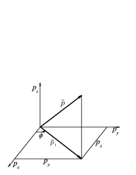
Figure 1: The particle momentum $\vec{p}$, in the Cartesian coordinate system,[$p_{x}$,$p_{y}$,$p_{z}$].

However, in experiment, the reaction plane is different event by event, thus the experimental measurement of elliptic flow is not trivial. One has to invoke a complex reaction plane identification method (two-particle correlation method) posk , cumulant method borg , or Lee-Yang zeroes method lee . In all of these methods a quantity has to be first constructed event by event: the event plane in posk , cumulant expansion of weighted $n$-$th$ transverse event-flow vector in borg , and a generating function in lee . Then a corresponding average over measured events has to be taken. Therefore the experimental extraction of elliptic flow parameter is event-wise average indeed.

The particle number (multiplicity) distribution can be expressed as

$$E{\frac{d^{3}N}{d^{3}p}}={\frac{d^{3}N}{p_{T}dydp_{T}d\phi}},$$ (2)

in the cylindrical coordinate system after substituting $p_{z}$ by y (rapidity) and using the relation of $dy/dp_{z}=1/E$ pdg . Then the normalized particle multiplicity distribution is

$${\frac{1}{N_{ev}}}{\frac{d^{3}N}{p_{T}dydp_{T}d\phi}},$$

$$N_{ev}=\int dy\int p_{T}dp_{T}\int d\phi{\frac{d^{3}N}{p_{T}dydp_{T}d\phi}},$$ (3)

where $N_{ev}$ is the event multiplicity and the integrals are taken over entire range of the variables.

This normalized particle multiplicity distribution in Eq.(3) is a three dimensional ($y,p_{T},\phi$) distribution function. The dimension can be reduced by integrating over a certain variable reic . For example, to study the $v_{n}$ as a function of rapidity $y$, $v_{n}(y)$, one should take integral over $p_{T}$, then above three dimensional distribution function reduces to a two dimensional distribution function

$${\frac{1}{N_{ev}}}{\int p_{T}dp_{T}\frac{d^{3}N}{p_{T}dydp_{T}d\phi}}.$$ (4)

In numerical calculations a small rapidity interval, $\Delta y$, is used instead of single $y$ value, the corresponding normalized particle multiplicity distribution becomes

$${\frac{1}{N_{evp}}}{\int_{p}dy^{\prime}\int p_{T}dp_{T}\frac{d^{3}N}{p_{T}dy^{\prime}dp_{T}d\phi}}$$

$$=\frac{d}{d\phi}[{\frac{1}{N_{evp}}}{\int_{p}dy^{\prime}\int p_{T}dp_{T}\frac{d^{2}N}{p_{T}dy^{\prime}dp_{T}}}]$$

$$\equiv f(\phi),$$

where

$$N_{evp}=\int_{p}dy^{\prime}\int p_{T}dp_{T}\int d\phi{\frac{d^{3}N}{p_{T}dy^{\prime}dp_{T}d\phi}},$$

and

$$\int_{p}dy^{\prime}\equiv\int_{y-\Delta y/2}^{y+\Delta y/2}dy^{\prime}.$$ (5)

Note that, the normalization factor $N_{evp}$ here is different from $N_{ev}$ in Eq. (3) in the range of integral over $y$ and is denoted as constrained event multiplicity. In the above equation $f(\phi)$ is the normalized distribution density function of $\phi$ and the $N_{evp}f(\phi)$ is the number of particles emitted into $d\phi$ at azimuthal angle $\phi$ without constraint on $p_{T}$ but $y$ is constrained in $\Delta y$. This can be constructed experimentally and/or calculated theoretically. Here we have taken $v_{n}(y)$ as an example but it is similar for the $v_{n}(p_{T})$.

Since $f(\phi)$ is $2\pi$ periodic and even function of $\phi$, it can be expanded by a fourier series beyer as

$$f(\phi)=\frac{1}{\pi}[\frac{1}{2}+\sum_{n=1}v_{n}cos(n\phi)],$$ (6)

$$v_{n}=\int d\phi f(\phi)cos(n\phi)$$

$$\hskip 142.26378pt\equiv\overline{cos(n\phi)}{\hskip 5.69046pt(n=1,2,...).}$$ (7)

In above equation, $\overline{cos(n\phi)}$ denotes the average of $cos(n\phi)$ over particles in a single event and can be calculated both experimentally and theoretically. The first expansion term, in Eq.(6), is a circle (isotropic), second term ($cos(\phi)$) a leave (directed flow), third term ($cos(2\phi)$) a four-leaved rose (elliptic flow), and the $(n+1)$-$th$ term ($cos(n\phi)$) a multi-leaved rose ($n$-$th$ harmonic) beyer .

As the event multiplicity fluctuates event-by-event, one always has to generate multiple events and to take average over events generated. So the $v_{n}$ in Eq.(7) should be

$$v_{n}^{e}=\langle\overline{cos(n\phi)}\rangle_{ev}{\hskip 5.69046pt(n=1,2,...),}$$ (8)

where $\langle...\rangle_{ev}$ means an average over all events. A superscript , “$e$”, is here added on $v_{n}$ to identify this average as the event-wise average. Applying recursion formula of cosine function beyer

$$cos(n\phi)=2cos((n-1)\phi)cos\phi-cos((n-2)\phi)$$ (9)

and

$$cos\phi=\frac{p_{x}}{p_{T}},\hskip 5.69046ptsin\phi=\frac{p_{y}}{p_{T}},$$ (10)

to Eq. (8), $v_{n}^{e}$ can be expressed as

$$v_{1}^{e}=\langle\overline{[\frac{p_{x}}{p_{T}}]}\rangle_{ev},\hskip 5.69046ptv_{2}^{e}=\langle\overline{[\frac{p_{x}^{2}-p_{y}^{2}}{p_{T}^{2}}]}\rangle_{ev},\hskip 5.69046pt....$$ (11)

Above deductions argued that the $v_{n}$ is an average of $cos(n\phi)$ first over particles in an event and then average over events (event-wise average) rather than a particle-wise average (“an average over all particles in all events” posk ) of $cos(n\phi)$. The particle-wise average of $cos(n\phi)$ can be expressed as

$$v_{n}^{p}=\langle\overline{cos(n\phi)}N_{evp}\rangle_{ev}/\langle N_{evp}\rangle_{ev}$$ (12)

(see Appendix). This is obviously different from the event-wise average. Only if the $\overline{cos(n\phi)}$ is independent of constrained event multiplicity $N_{evp}$ (i. e. constrained multiplicity plays no role in the average) the $v_{n}^{p}$ reduces to $v_{n}^{e}$. In fact, the $\overline{cos(n\phi)}$ and $N_{evp}$ correlate (even negatively correlate) with each other. This is because the larger event multiplicity is due to more central collision (larger overlap zone between colliding nuclei) and the larger overlap zone in turn leads to less azimuthal asymmetry. The particle-wise average does not take the influence of event multiplicity into account, thus it is inaccurate from physics point of view. Of course, for very narrow multiplicity (centrality) bins the particle-wise average is not very problematic. However for the wide multiplicity bins (such as the 0-40% most central Au+Au collisions studied in phob3 and/or the minimum bias Au+Au collision data given in star2 ) that correction is not negligible.

We have applied the parton and hadron cascade model, PACIAE sa1 , to calculate the charged hadron $v_{2}(\eta)$ in 0-40% most central $Au+Au$ collisions at $\sqrt{s_{NN}}$=200 GeV by the method of event-wise and particle-wise averages separately. The $v_{2}^{e}(\eta)$ calculated by event-wise average is about 10% larger than $v_{2}^{p}(\eta)$ calculated by particles-wise average. This means that $\langle\overline{cos(n\phi)}N_{evp}\rangle_{ev}$ is smaller than $\langle\overline{cos(n\phi)}\rangle_{ev}\langle N_{evp}\rangle_{ev}$, i. e. there is a negative correlation between $\overline{cos(n\phi)}$ and $N_{evp}$. This is consistent with the physical picture given in the last paragraph.

In summary we have rederived the elliptic flow and other harmonics in fourier expansion of the particle momentum azimuthal distribution starting from the particle number (multiplicity) distribution in the momentum space. It is argued that the parameter of $n-th$ harmonic, $v_{n}$, should be calculated as an average of $con(n\phi)$ first over particles in an event and then over events (event-wise average). This is different from the particle-wise average (“an average over all particles in all events”) of $cos(n\phi)$. In case of large centrality (multiplicity) bin the particle-wise average is not accurate because the influence (fluctuation) of particle multiplicity is not taken into account.

Appendix

In this appendix the variables are assumed to be discrete for simplicity. Then the particle-wise average of $cos(n\phi)$ can be expressed as

$$v_{n}^{p}=\frac{\sum\limits_{k}[cos(n\phi)]_{k}}{\sum\limits_{k}1},$$ (13)

where $\sum\limits_{k}$ denotes the sum over all particles in all events. If the summation, both in numerator and denominator, groups according to event (denoted by $j$) then

$$v_{n}^{p}=\frac{\sum\limits_{j}[\sum\limits_{i\in j}[cos(n\phi)]_{i}]}{\sum\limits_{j}(N_{evp})_{j}},$$ (14)

where $\sum\limits_{j}$ is the sum over events and $\sum\limits_{i\in j}$ denotes the sum over particles in the $j$-$th$ event. According to the definition of average over particle in a single event beyer the $v_{n}^{p}$ can be further expressed as

$$v_{n}^{p}=\frac{\sum\limits_{j}(\overline{cos(n\phi)})_{j}(N_{evp})_{j}}{\sum\limits_{j}(N_{evp})_{j}}$$

$$=\frac{\langle\overline{cos(n\phi)}N_{evp}\rangle_{ev}}{\langle N_{evp}\rangle_{ev}}.$$ (15)

Acknowledgment

We thank L. P. Csernai for valuable discussions. The financial supports from the NSFC (10475032, 10605040, and 10635020) in China and the NSFC (China)/NFR (Norway) collaboration are gratefully acknowledged.

References

- (1) M. Gyulassy, nucl-th/0403032.
- (2) M. Gyulassy and X.-N. Wang, Comput. Phys. Commun. 83, 307 (1994).
- (3) P. F. Kolb, P. Huovinen, U. W. Heiz, and H. Heiselberg, Phys. Lett. B 500, 232 (2001).
- (4) B. B. Back, et al., Phobos collaboration, Phys. Rev. C 72, 051901(R) (2005).
- (5) W. A. Zajc, arXiv:0802.3552.
- (6) B. I. Abelev, STAR collaboration, Phys. Rev. Lett. 99, 112301 (2007), and references therein.
- (7) S. S. Adler, et al., PHENIX collaboration, Phys. Rev. Lett. 99, 052301 (2007), and references therein.
- (8) B. Alver, et al., PHOBOS collaboration, Phys. Rev. Lett. 98, 242302 (2007), and references therein.
- (9) Bin Zhang, M. Gyulassy, and Che-Ming Ko, Phys. Lett. B 455, 45 (1999).
- (10) E. E. Zabrodin, C. Fuchs, L. V. Bravina, and A. Faessler, Phys. Lett. B 508, 184 (2001).
- (11) Lie-Wen Chen, V. Greco, Che-Ming Ko, and P. F. Kolb, Phys. Lett. B 605, 95 (2005).
- (12) Zhe Xu, C. Greiner, and H. Stöcker, arxiv:0711.0961.
- (13) Xianglei Zhu, M. Bleicher, and H. Stöcker, Phys. Rev. C 72, 064911 (2005).
- (14) S. A. Voloshin and Y. Zhang, Z. Phys. C 70, 665 (1996).
- (15) A. M. Poskanzer and S. A. Voloshin, Phys. Rev. C 58, 1671 (1998).
- (16) N. Borghini, P. M. Dinh, and J.-Y. Ollitrault, Phys. Rev. C 63, 054906 (2001).
- (17) R. S. Bhalerao, N. Borghini, J.-Y. Ollitrault, Nucl. Phys. A 727, 373 (2003).
- (18) PDG, “Particle Physics Booklet”, Extracted from C. Amsler, et al., Phys. Lett. B 667, 1 (2008).
- (19) L. E. Reichl, “A Modern Course in Statistical Physics”, p.144, University of Texas Press, Austin, 1980.
- (20) W. H. Beyer, CRC, Standard mathematical table and formulae, 29th Edition, 1991.
- (21) B. B. Back, et al., Phobos collaboration, Phys. Rev. Lett. 94, 122303 (2005).
- (22) J. Adams, et al., STAR collaboration, Phys. Rev. Lett. 92, 062301 (2004).
- (23) Ben-Hao Sa, Xiao-Mei Li, Shou-Yang Hu, Shou-Ping Li, Jing Feng, and Dai-Mei Zhou, Phys. Rev. C 75, 054912 (2007).