Hyperbolic attractor of Smale-Williams type in a system of two coupled non-autonomous amplitude equations

Abstract

Recently, a system with uniformly hyperbolic attractor of Smale-Williams type has been suggested [Kuznetsov, Phys. Rev. Lett., 95, 144101, 2005]. This system consists of two coupled non-autonomous van der Pol oscillators and admits simple physical realization. In present paper we introduce amplitude equations for this system and prove that the attractor of the system of amplitude equations is also uniformly hyperbolic. Also we represent qualitative illustrations as well as quantitative characteristics of a chaotic dynamics on this attractor.

1 Introduction

One of the interesting problems in nonlinear dynamics is a development of physical applications of the hyperbolic theory. A trajectory in phase space of a dynamical system is hyperbolic when a tangent vector space on each its point can be described as a direct sum of subspaces spanned on stable and unstable perturbation vectors and this representation is invariant along the trajectory. Dissipative system with attractor containing only hyperbolic trajectories demonstrates strong chaotic properties and permits advanced mathematical analysis. Monographs and textbooks on nonlinear dynamics provide examples of such attractors, but most of them are artificial mathematical constructions like Plykin attractor and Smale-Williams solenoid [22, 8, 7, 21, 10, 2, 17, 3]. On the other hand, attractors of realistic systems with complicated dynamics, like the Lorenz model [1, 16], do not relate to the class of uniformly hyperbolic, so the hyperbolic theory can not be applied to them in corpore.

In a recent paper [13] one of the authors suggested an implementation of the Smale-Williams attractor in a system of two coupled non-autonomous van der Pol oscillators with natural frequencies relating as 1:2. Subsystems are activated alternately due to a slow variation of their excitation parameters by an external force. The excitation is passed from one oscillator to another, so that a phase of the oscillations is doubled within each full cycle. This system was realized as an electronic devise and studied experimentally [12]. Assumption about the hyperbolicity of the attractor was based on the fact that a phase of one of the oscillators, being measured at successive stages of its excitation, was obeyed to the Bernoulli map, as must be for the Smale-Williams attractor. Moreover, computations revealed a robustness of the attractor: Its Cantor-like transverse structure and positive Lyapunov exponent were insensitive to variations of parameters in the equations. Further analysis [11] showed that 4D phase space of a Poincaré map, describing a successive states of the system over a period of the external forcing, contains a toroidal absorbing domain (a direct product of 1D circle and 3D ball) that is mapped into itself according to the Smale-Williams procedure. Performed numerical analysis proved the validity of sufficient conditions of the hyperbolicity that are formulated in terms of expanding and contracting cones in tangent vector space.

An idea of alternate excitation of two oscillators that pass the excitation from one to another can be applied to amplitude equations which are derived for the van der Pol equations via the method of slow varying amplitudes. Actually, equations of this type can be obtained for a wide variety of dynamical systems because, in fact, they correspond to a normal form of Andronov-Hopf bifurcation of birth of a limit cycle. For example, amplitude equations are employed in Landau’s theory of turbulence [15, 14].

Reasoning in the manner of Landau’s theory, we can assume that a spatially extended system have two modes with frequencies relating as 1:2. Some additional periodic and slow component acts on these modes so that they excite alternately and pass the excitation from one to another through a nonlinear coupling. Then, according to the idea of [13], this can result in the formation of a hyperbolic attractor of Smale-Williams type.

This paper is devoted to a study of a system of two coupled non-autonomous amplitude equations. We provide a proof of hyperbolicity of an attractor of this system and also discuss some attributes of its hyperbolic dynamics.

2 System of two coupled non-autonomous van der Pol oscillators and corresponding amplitude equations

The starting point of our analysis is a system of two coupled van der Pol oscillators that has been proposed in [13]:

$$\begin{gathered}\ddot{x}-[A\cos(2\pi\tau/P)-x^{2}]\dot{x}+\omega_{0}^{2}x=\varepsilon y\cos\omega_{0}\tau,\\ \ddot{y}-[-A\cos(2\pi\tau/P)-y^{2}]\dot{y}+4\omega_{0}^{2}y=\varepsilon x^{2},\end{gathered}$$ (1)

where $\tau$ denotes time. The oscillators have natural frequencies $\omega_{0}$ and $2\omega_{0}$, respectively. Their bifurcation parameters controlling a birth of a limit cycle undergo a variation with a period $P$ and amplitude $A$. The variations are in counter phases: when the first oscillator is excited the second one is not and vice versa. The forcing is supposed to be slow, i.e., its period is much larger than natural periods of the oscillators. The oscillators are coupled and the intensity of this interaction is controlled by a parameter $\varepsilon$.

The subject of our study shall be a system of amplitude equations corresponding to Eqs (1). To derive these equation we follow the standard technic and assume a solution to Eqs (1) to be oscillations with frequencies $\omega_{0}$ and $2\omega_{0}$, respectively, and with slow varying complex amplitudes:

$$\begin{gathered}x(\tau)=a(\tau)e^{i\omega_{0}\tau}+a^{*}(\tau)e^{-i\omega_{0}\tau},\\ y(\tau)=b(\tau)e^{2i\omega_{0}\tau}+b^{*}(\tau)e^{-2i\omega_{0}\tau}.\end{gathered}$$ (2)

Upper index “*” means complex conjugation. The derivatives of complex amplitudes $a$ and $b$ should satisfy additional conditions

$$\begin{gathered}\dot{a}e^{i\omega_{0}\tau}+\dot{a}^{*}e^{-i\omega_{0}\tau}=0,\\ \dot{b}e^{2i\omega_{0}\tau}+\dot{b}^{*}e^{-2i\omega_{0}\tau}=0.\end{gathered}$$ (3)

Taking these conditions into account we substitute (2) into (1) and average over the period $2\pi/\omega_{0}$. Because the complex amplitudes $a$ and $b$ are supposed to be slow, the resulting equations have the form:

$$\begin{gathered}\dot{a}=(A/2)a\cos(2\pi\tau/P)-|a|^{2}a/2-i\varepsilon b/(4\omega_{0}),\\ \dot{b}=-(A/2)b\cos(2\pi\tau/P)-|b|^{2}b/2-i\varepsilon a^{2}/(4\omega_{0}).\end{gathered}$$ (4)

These equations allows the following rescaling of time variable and parameters:

$$t=\tau/2,\;T=P/2,\;\epsilon=\varepsilon/2\omega_{0}.$$ (5)

As a result, we obtain a sought system of amplitude equations:

$$\begin{gathered}\dot{a}=Aa\cos(2\pi t/T)-|a|^{2}a-i\epsilon\,b,\\ \dot{b}=-Ab\cos(2\pi t/T)-|b|^{2}b-i\epsilon\,a^{2}.\end{gathered}$$ (6)

To clarify the nature of dynamics of the system (6), we consider a behavior of amplitudes and phases of complex variables $a$ and $b$. Define phases within the interval $[0,2\pi)$: $\phi=\arg a$, $\psi=\arg b$. Suppose that the first oscillator is excited and its amplitude $|a|$ is high. Hence, the second one is suppressed so its amplitude $|b|$ is small. The coefficients in Eqs. (6) are real except the coupling. It means that the phases can be changed only as a result of interaction between subsystems. But when $a$ is excited $|b|$ is small and its action on $a$ is negligible. Thus, the phase of $a$ remains constant during the excitation stage. The opposite influence from $a$ to $b$ is high and the coupling term is proportional to $a^{2}$. It means that after a half period $T/2$ at the threshold of its own excitation the oscillator $b$ inherits a doubled phase of $a$ (the phase also gets a shift $-\pi/2$ because of the imaginary unit at the coupling term). Now the roles of the subsystems are exchanged. The phase of $b$ remains constant when this subsystem is excited and at the end, after the other half period $T/2$, the phase is returned back to $a$ through a linear coupling term (also with the shift $-\pi/2$). As a result, the first oscillator $a$ doubles its phase during the period $T$.

Fig. 1 demonstrates a numerical solution to Eqs. (6) illustrating these considerations. Here and below the solutions are obtained via Runge-Kutta method of the fifth order with a step-size control [19]. Panel (a) demonstrates an alternate excitation of the subsystems $a$ and $b$. Notice, that each time the amplitude $|a|$ attains its maximum, the height of the maximum is a bit different from the previous one. The same is for the amplitude $|b|$. This is a manifestation of a chaotic nature of the discussed dynamics. Panel (b) represents a time dependance of a complex variable $a$. We observe a series of spikes corresponding to the stages of the excitation of $a$. Projections of spikes on the plane $\{\mathop{\mathrm{Re}}a$, $\mathop{\mathrm{Im}}a\}$ are almost straight lines. This confirms our previous conclusion that the phase of an excited subsystem, i.e., an angle between the projection and the real axis $\mathop{\mathrm{Re}}a$, remains constant or, at least, almost constant. This panel also illustrates the phase doubling after each period $T$: compare angles between spikes $4$, $5$ and $6$.

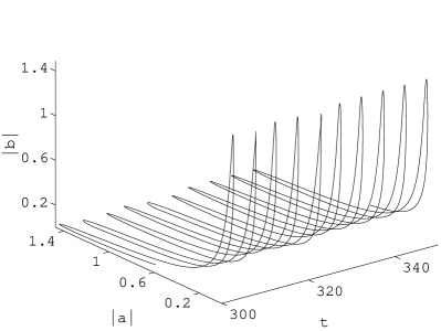
a)b)

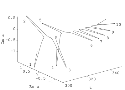
Figure 1: Illustration of a dynamics of the system (6): alternate excitation and decay of the components $a$ and $b$ (panel (a)) and time dependance of real and imaginary parts of $a$ (panel (b)). Observe that being excited the component $a$ has almost constant phase, but the phase is doubled at every new stage of the excitation (compare, for example, spikes labelled $4$, $5$ and $6$).

The above discussion allows us to write down a map for a series of phases $\phi_{n}=\arg a(nT)$ that are measured over the time step $T$:

$$\phi_{n+1}=2\phi_{n}-\pi\mod 2\pi.$$ (7)

Up to a constant addition (that can be eliminated by a shift of the origin of the phase) this map coincides with the well known Bernoulli map [20]. It demonstrates a chaotic dynamics and the chaos is homogeneous: a rate of exponential divergence of two close trajectories is identical in each point of the phase space and equal to $\ln 2$.

Fig. 2 show $\phi_{n+1}=\arg a(nT+T)$ vs. $\phi_{n}=\arg a(nT)$ computed numerically for the system (6). One can see a very high correspondence with the map (7). The most important point is the topological equivalence between the empirical map and the Bernoulli map: one full circle that passes a preimage (i.e., turn of a phase on $2\pi$) implies two passes of a circle for an image ($4\pi$ turn of a phase).

Figure 2: Numerically computed map for the phase $\phi_{n}=\arg a(nT)$ measured over the time step $T$ at $A=3$, $T=5$ and $\epsilon=0.05$.

The correspondence with the Bernoulli map presumes that among Lyapunov exponents of the system (6) the one should be equal to $\ln 2/T$. To compute the Lyapunov exponents we employ the Benettin’s algorithm [5, 18] that requires to solve simultaneously Eqs. (6) and four sets of linearized equations for small perturbations:

$$\begin{gathered}\delta\dot{x}_{0}=A\cos(2\pi t/T){\delta x_{0}}-(3x_{0}^{2}+x_{1}^{2}){\delta x_{0}}-2x_{0}x_{1}{\delta x_{1}}+\epsilon{\delta x_{3}},\\ \delta\dot{x}_{1}=A\cos(2\pi t/T){\delta x_{1}}-(x_{0}^{2}+3x_{1}^{2}){\delta x_{1}}-2x_{0}x_{1}{\delta x_{0}}-\epsilon{\delta x_{2}},\\ \delta\dot{x}_{2}=-A\cos(2\pi t/T){\delta x_{2}}-(3x_{2}^{2}+x_{3}^{2}){\delta x_{2}}-2x_{2}x_{3}{\delta x_{3}}+2\epsilon(x_{0}{\delta x_{1}}+x_{1}{\delta x_{0}}),\\ \delta\dot{x}_{3}=-A\cos(2\pi t/T){\delta x_{3}}-(x_{2}^{2}+3x_{3}^{2}){\delta x_{3}}-2x_{2}x_{3}{\delta x_{2}}-2\epsilon(x_{0}{\delta x_{0}}-x_{1}{\delta x_{1}}),\end{gathered}$$ (8)

where $x_{0}=\mathop{\mathrm{Re}}a$, $x_{1}=\mathop{\mathrm{Im}}a$, $x_{2}=\mathop{\mathrm{Re}}b$, $x_{3}=\mathop{\mathrm{Im}}b$, and $\delta x_{0}$, $\delta x_{1}$, $\delta x_{2}$, $\delta x_{3}$ denotes small perturbations to these values. Before the start of the computations, we initialize each set of linearized equations by a unit perturbation vector, so that four these vectors comprise an orthogonal system. Advancing the solution, we perform the Gram-Schmidt orthogonalization [18] of these vectors after each time interval $T$ and normalize them to prevent a numerical overflow. Four Lyapunov exponents $\lambda_{k}$ appear as time averaged logarithms of norms of the perturbation vectors. Finally, we multiply the computed values on $T$, to obtain the Lyapunov exponents for corresponding map, describing the dynamics of the system with time step $T$: $\Lambda_{k}=\lambda_{k}T$

Fig. 3 demonstrates the exponents $\Lambda_{k}$ as functions of the parameter $A$. The largest exponent is positive for a wide range of parameter values. This is the evidence of a chaotic nature of the observed dynamics. Three others are always negative. For example, at $A=3$ the Lyapunov exponents are $\Lambda_{1}\approx 0.691$, $\Lambda_{2}\approx-4.06$, $\Lambda_{3}\approx-6.48$, and $\Lambda_{4}\approx-9.06$. As typical for maps and non-autonomous continuous time systems, a zero exponent is absent. The largest exponent is close to $\ln 2$. This corresponds to our qualitative conclusion that the dynamics of the phase of $a$ is obeyed, to some degree of accuracy, by the Bernoulli map (7). Also notice that the largest exponent is almost independent on $A$, and the others vary rather smoothly, without peaks and canyons. This can be treated as a manifestation of a robustness of the observed chaotic oscillations which, in turn, indicates a hyperbolic nature of an underlying chaotic attractor.

Figure 3: Lyapunov exponents $\Lambda_{k}$ vs. parameter $A$ for the system (6) at $T=5$ and $\epsilon=0.05$. Dash lines indicate corresponding Lyapunov exponents for the initial system (1) at $P=10$, $\omega_{0}=2\pi$ and $\varepsilon=0.2\pi$.

This behavior of Lyapunov exponents agrees very well with the behavior of the exponents of the initial system of two van der Pol oscillators (1) [13, 12]. In Fig. 3 the Lyapunov exponents of the initial system are plotted by dashed lines. Values of parameters, being recalculated as required by Eq. (5), correspond to the parameters of the system (6). The largest Lyapunov exponents of two systems are almost identical and three others pairs are also close to each other. We treat this good correspondence between the initial system and the approximate amplitude equation as one more demonstration of a robustness. In turn, the robustness is related to a hyperbolic nature of the observed dynamics.

3 Stroboscopic Poincaré map and absorbing domain

Consider our system (6) in a certain time moment $t_{n}=nT$. Its instantaneous state is given by a vector $\mathbf{x}_{n}=\{\mathop{\mathrm{Re}}a(t_{n}),\mathop{\mathrm{Im}}a(t_{n}),\mathop{\mathrm{Re}}b(t_{n}),\mathop{\mathrm{Im}}b(t_{n})\}$. If we take this vector as an initial state and integrate the equations over the period $T$, we find a new vector $\mathbf{x}_{n+1}=\{\mathop{\mathrm{Re}}a(t_{n+1}),\mathop{\mathrm{Im}}a(t_{n+1}),\mathop{\mathrm{Re}}b(t_{n+1}),\mathop{\mathrm{Im}}b(t_{n+1})\}$. This vector is unambiguously determined by the vector $\mathbf{x}_{n}$. Hence, we can define a mapping that operates in $\mathbb{R}^{4}$:

$$\mathbf{x}_{n+1}=\mathrm{\mathbf{T}}(\mathbf{x}_{n}).$$ (9)

This equation defines a stroboscopic Poincaré map for the system (6). From a geometric point of view, each vector $\mathbf{x}_{n}$ belongs to a 4D hyperplane $t=t_{n}=nT$ which is a section of a flow of trajectories in the 5D extended phase space $\{\mathop{\mathrm{Re}}a,\mathop{\mathrm{Im}}a,\mathop{\mathrm{Re}}b,\mathop{\mathrm{Im}}b,t\}$. Because of periodicity of the phase in $t$, these hyperplanes can be identified. So, we can say that Eq. (9) maps 4D hyperplane $\{\mathop{\mathrm{Re}}a,\mathop{\mathrm{Im}}a,\mathop{\mathrm{Re}}b,\mathop{\mathrm{Im}}b\}$ onto itself.

The map $\mathrm{\mathbf{T}}$ is generated by differential equations whose right-hand sides are smooth and limited within a finite region of $a$ and $b$. According to the existence, uniqueness, continuity and differentiability theorems, the map $\mathrm{\mathbf{T}}$ is one-to-one diffeomorphism belonging to class $C^{\infty}$) [4].

In course of iterations, the map $\mathbf{x}_{n+1}=\mathrm{\mathbf{T}}(\mathbf{x}_{n})$ expands a volume element in a direction, associated with the phase $\phi$, see Eq. (7), while three others directions are contracting. Taking into account a periodicity of the phase, we can consider a 4D toroid which is a direct product of a 1D circle and 3D ball. One iteration of the map corresponds to a longitudinal stretch and transverse contraction of this object followed by its kinking and insertion into the initial area as a double loop. This exactly corresponds to the Smale and Williams procedure except that our map is embedded into 4D rather then 3D state space.

Mentioned toroid with its interior is an absorbing domain which we denote as $U$. Points, belonging to this area, fall into the interior of $U$ under the action of the map $\mathrm{\mathbf{T}}$: $\mathrm{\mathbf{T}}(U)\subset\mathop{\mathrm{Int}}U$. An attractor may be defined as an intersection of all images of $U$, generated by successive iterations of $\mathrm{\mathbf{T}}$: $A=\bigcap_{\,n=1}^{\,\infty}\mathrm{\mathbf{T}}^{n}(U)$.

Consider the space $\{\mathop{\mathrm{Re}}a,\mathop{\mathrm{Im}}a,\mathop{\mathrm{Re}}b,\mathop{\mathrm{Im}}b\}$ and define a torus as

$$(|a|-r)^{2}+|b|^{2}=(\chi d)^{2}.$$ (10)

Here $r$ denotes a radius of the 1D circle, and $\chi d$ is a radius of the 3D ball that appears in a radial section of the torus by a hyperplane perpendicular to the circle. Parameter $\chi$ is introduced to scan points both on the surface ($\chi=1$) and inside the absorbing domain, $0\leq\chi\leq 1$. The torus (10) can also be defined parametrically via the equations

$$\begin{gathered}\mathop{\mathrm{Re}}a=(\chi d\cos\theta+r)\cos\phi,\;\mathop{\mathrm{Re}}b=\chi d\sin\theta\cos\psi,\\ \mathop{\mathrm{Im}}a=(\chi d\cos\theta+r)\sin\phi,\;\mathop{\mathrm{Im}}b=\chi d\sin\theta\sin\psi.\end{gathered}$$ (11)

Here parameters $\phi$ and $\psi$ can be treated as phases of $a$ and $b$, respectively.

Numerical values of $r$ and $d$ should be found for the attractor to be fitted inside the torus. Consider specific values of the parameters of the system, say, $A=3$, $T=5$, $\epsilon=0.05$, and compute a large amount of points belonging to the attractor of the map (9). Projections of these points to the plane $\{\mathop{\mathrm{Re}}a,\mathop{\mathrm{Im}}a\}$ fall somewhere in a vicinity of a circle whose radius $r$ can be found as a mean amplitude $|a|$ of these points. For our specific parameters we find $r=0.631166$.

To compute $d$, let us consider a series of tori parameterized by the section radius $d_{x}$ that grows from $0$ with some small step (we assume here that $\chi=1$). All the tori have identical radiuses $r$. For each $d_{x}$ we cover the surface of a corresponding torus by a mesh, using parametric Eqs. (11). In our computations the angle variables $\phi$, $\psi$ and $\theta$ were varied with the step $2\pi/50$. The map (9) is iterated once form each node of the mesh. An image point falls on the surface of a new torus whose section radius is equal to $\sqrt{(|a|-r)^{2}+|b|^{2}}$, where $|a|$ and $|b|$ are related here to the image point. Thus, the torus $d_{x}$ generates a set of “image” tori. Because we are seeking for an absorbing domain, we must take the worst case, i.e., the image torus with the largest section radius. Denoting this radius as $d_{y}$, we obtain a function $d_{y}=F(d_{x})$ that is plotted in Fig. 4. This function monotonously grows and meets the line $d_{y}=d_{x}$ at $d_{x}\approx 0.0918$. All tori to the right from this point can be taken as an absorbing domain because their surfaces, as well as the interior, are mapped into their interior. We take a torus whose section radius $d$ is about $1\%$ above the intersection point. So, the set of parameters of the system and corresponding parameters of the absorbing domain are the following:

$$\begin{gathered}A=3,\;T=5,\;\epsilon=0.05,\\ r=0.631166,\;d=0.0927.\end{gathered}$$ (12)

Fig. 5 demonstrates 3D view of the absorbing domain with an enclosed attractor. Points of the attractor are project from 4D space $\{\mathop{\mathrm{Re}}a,\mathop{\mathrm{Im}}a,\mathop{\mathrm{Re}}b,\allowbreak\mathop{\mathrm{Im}}b\}$ along axis $\mathop{\mathrm{Im}}b$ onto the section plane $\psi=0$.

Figure 4: Selection of the parameters of an absorbing domain (see explanations in the text).

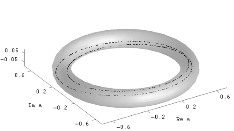
Figure 5: 3D projection of a toroidal absorbing domain and enclosed attractor of the Poincaré map (9).

4 Sufficient condition for hyperbolicity: general formulation of a method

To verify hyperbolic nature of the attractor of the system (6), we shall follow the method developed in [11] for the attractor of two non-autonomous van der Pol oscillators (1). In this section we reproduce the details of this method.

The central point is the theorem on expanding and contracting cones [22, 10, 9]. Unlike the general case, it is sufficient here to deal with a diffeomorphism of class $C^{\infty}$ in the Euclidian space $\mathbb{R}^{4}$, namely, we consider the Poincaré map $\mathrm{\mathbf{T}}(\mathbf{x})$. Let $\mathrm{\mathbf{DT}}_{x}$ be the Jacobi matrix of the map $\mathbf{x}^{\prime}=\mathrm{\mathbf{T}}(\mathbf{x})$ at $\mathbf{x}$: $\mathrm{\mathbf{DT}}_{x}=\{\partial x_{i}^{\prime}/\partial x_{j}\}$, $i,j=0,1,2,3$, and let $\mathrm{\mathbf{DT}}_{x}^{-1}$ designates the derivative matrix for the inverse map $\mathrm{\mathbf{T}}^{-1}(x)$. Also, let $\delta\mathbf{x}$ denotes the vector of a small perturbation to $\mathbf{x}$. In a linear approximation the evolution of a perturbed state $\mathbf{x}+\delta\mathbf{x}$ corresponds to transformation of the vector $\delta\mathbf{x}$ according to a linear mapping $\delta\mathbf{x}^{\prime}=\mathrm{\mathbf{DT}}_{x}\delta\mathbf{x}$. Vectors $\delta\mathbf{x}$ form a tangent space $\mathbb{V}_{x}$ associated with $\mathbf{x}$.

Theorem ([22, 10, 9])

Suppose that a diffeomorphism $\mathrm{\mathbf{T}}$ of class $C^{\infty}$ maps a bounded domain $U\subset\mathbb{R}^{4}$ into itself: $\mathrm{\mathbf{T}}(U)\subset\mathop{\mathrm{Int}}U$, and $A\subset\mathop{\mathrm{Int}}U$ is an invariant set for the diffeomorphism. The set $A$ will be uniformly hyperbolic if there exists a constant $\gamma>1$ and the following conditions hold:

1. The expanding and contracting cones $S_{x}^{\gamma}$ and $C_{x}^{\gamma}$ may be defined in the tangent space $\mathbb{V}_{x}$ at each $\mathbf{x}\in A$, such that $||\mathrm{\mathbf{DT}}_{x}\mathbf{u}||\geq\gamma||\mathbf{u}||$ for all $\mathbf{u}\in S_{x}^{\gamma}$, and $||\mathrm{\mathbf{DT}}_{x}^{-1}\mathbf{v}||\geq\gamma||\mathbf{v}||$ for all $\mathbf{v}\in C_{x}^{\gamma}$; moreover, for all $\mathbf{x}\in A$ they satisfy $S_{x}^{\gamma}\cap C_{x}^{\gamma}=\varnothing$ and $S_{x}^{\gamma}+C_{x}^{\gamma}=\mathbb{V}_{x}$.

2. The cones $S_{x}^{\gamma}$ are invariant with respect to action of $\mathrm{\mathbf{DT}}$, and $C_{x}^{\gamma}$ are invariant with respect to action of $\mathrm{\mathbf{DT}}^{-1}$, i.e., for all $x\in A$ $\mathrm{\mathbf{DT}}_{x}(S_{x}^{\gamma})\subset S_{\mathrm{\mathbf{T}}(x)}^{\gamma}$ and $\mathrm{\mathbf{DT}}_{x}^{-1}(C_{x}^{\gamma})\subset C_{\mathrm{\mathbf{T}}^{-1}(x)}^{\gamma}$.

If the formulated conditions are valid for all points of the absorbing domain $U$, they are obviously true for the attractor $A\subset U$. Therefore, the following procedure can be performed for a verification of the conditions of the theorem.

Starting at $\mathbf{x}=\{\mathop{\mathrm{Re}}a,\mathop{\mathrm{Im}}a,\mathop{\mathrm{Re}}b,\mathop{\mathrm{Im}}b\}\in U$, we solve Eqs. (6) numerically on the interval $t\in[0,T]$ and get the image $\mathbf{x}^{\prime}=\mathrm{\mathbf{T}}(\mathbf{x})$. Also, we initialize four sets of equations for small perturbations (8) with unit vectors $\{1,0,0,0\}$, $\{0,1,0,0\}$, $\{0,0,1,0\}$ and $\{0,0,0,1\}$, respectively, and solve these equations simultaneously with the original system. From the resulting four vector-columns we compose a matrix $\mathrm{\mathbf{U}}=\mathrm{\mathbf{DT}}_{x}$.

If the Poincaré map is iterated one time from $\mathbf{x}$, any perturbation vector $\mathbf{u}$ transforms to $\mathbf{u}^{\prime}=\mathrm{\mathbf{U}}\mathbf{u}$. A squared Euclidean norm of this vector is $||\mathbf{u}^{\prime}||^{2}=\mathbf{u}^{\mathrm{T}}\mathrm{\mathbf{U}}^{\mathrm{T}}\mathrm{\mathbf{U}}\mathbf{u}$ where $\mathrm{T}$ means the transposition. Via the inverse matrix $\mathrm{\mathbf{U}}^{-1}$ we can write $\mathbf{u}=\mathrm{\mathbf{U}}^{-1}\mathbf{u}^{\prime}$ and $||\mathbf{u}||^{2}=\mathbf{u}^{\prime\,\mathrm{T}}\mathrm{\mathbf{U}}^{-1,\mathrm{T}}\mathrm{\mathbf{U}}^{-1}\mathbf{u}^{\prime}$. A condition that the preimage of $\mathbf{u}^{\prime}$ relates to the expanding cone $S_{x}^{\gamma}$ is an inequality $||\mathbf{u}^{\prime}||\geq\gamma||\mathbf{u}||$, or

$$\mathbf{u}^{\prime\,\mathrm{T}}\mathrm{\mathbf{H}}_{\gamma}\mathbf{u}^{\prime}\leq 0,$$ (13)

where $\mathrm{\mathbf{H}}_{\gamma}=\mathrm{\mathbf{U}}^{-1,\mathrm{T}}\mathrm{\mathbf{U}}^{-1}-\gamma^{-2}$.

If we start from $\mathbf{x}^{\prime}=\mathrm{\mathbf{T}}(\mathbf{x})$, a vector $\mathbf{u}^{\prime}$ transforms to $\mathbf{u}^{\prime\prime}=\mathrm{\mathbf{U}}^{\prime}\mathbf{u}^{\prime}$, and we have $||\mathbf{u}^{\prime\prime}||^{2}=\mathbf{u}^{\prime\,\mathrm{T}}\mathrm{\mathbf{U}}^{\prime\,\mathrm{T}}\mathrm{\mathbf{U}}^{\prime}\mathbf{u}^{\prime}$. The expanding cone $S_{\mathrm{\mathbf{T}}(x)}^{\gamma}$ at $\mathbf{x}^{\prime}=\mathrm{\mathbf{T}}(\mathbf{x})$ is determined by an inequality $||\mathbf{u}^{\prime\prime}||\geq\gamma||\mathbf{u}^{\prime}||$, or

$$\mathbf{u}^{\prime\,\mathrm{T}}\mathrm{\mathbf{H}}_{\gamma}^{\prime}\mathbf{u}^{\prime}\geq 0,$$ (14)

where $\mathrm{\mathbf{H}}_{\gamma}^{\prime}=\mathrm{\mathbf{U}}^{\prime\,\mathrm{T}}\mathrm{\mathbf{U}}^{\prime}-\gamma^{2}$.

Thus, the required condition $\mathrm{\mathbf{DT}}_{x}(S_{x}^{\gamma})\subset S_{\mathrm{\mathbf{T}}(x)}^{\gamma}$ is formulated in terms of two quadratic forms: If the inequality (13) holds, then the inequality (14) must be valid too.

Let us perform a canonical reduction of the quadratic form $\mathbf{u}^{\prime\,\mathrm{T}}\mathrm{\mathbf{H}}_{\gamma}^{\prime}\mathbf{u}^{\prime}$ by a coordinate change. Because the matrix $\mathrm{\mathbf{U}}^{\prime\,\mathrm{T}}\mathrm{\mathbf{U}}^{\prime}$ is real and symmetric, an orthonormal basis of eigenvectors $\mathbf{d}_{0}$, $\mathbf{d}_{1}$, $\mathbf{d}_{2}$, $\mathbf{d}_{3}$ may be chosen. Then, the matrix $\mathrm{\mathbf{D}}=\{\mathbf{d}_{0},\mathbf{d}_{1},\mathbf{d}_{2},\mathbf{d}_{3}\}$ is a diagonalizer: $\mathrm{\mathbf{D}}^{\mathrm{T}}\mathrm{\mathbf{U}}^{\prime\,\mathrm{T}}\mathrm{\mathbf{U}}^{\prime}\mathrm{\mathbf{D}}=\{\Lambda_{i}^{2}\delta_{ij}\}$, $i,j=0,1,2,3$. The eigenvalues on the diagonal $\Lambda_{i}^{2}$ are supposed to be arranged in the decreasing order. In our case there will be one stretching and three contracting directions, so, $\Lambda_{0}^{2}>1$, $\Lambda_{1,2,3}^{2}<1$. Let $\gamma$ be selected in such a way that $\Lambda_{0}^{2}>\gamma^{2}$, $\Lambda_{1,2,3}^{2}<\gamma^{2}$. Under the transformation $\mathrm{\mathbf{D}}$ the matrix $\mathrm{\mathbf{H}}_{\gamma}^{\prime}$ also becomes a diagonal:

$$\mathrm{\mathbf{D}}^{\mathrm{T}}\mathrm{\mathbf{H}}_{\gamma}^{\prime}\mathrm{\mathbf{D}}=\mathrm{\mathbf{D}}^{\mathrm{T}}(\mathrm{\mathbf{U}}^{\prime\,\mathrm{T}}\mathrm{\mathbf{U}}^{\prime}-\gamma^{2})\mathrm{\mathbf{D}}=\{(\Lambda_{i}^{2}-\gamma^{2})\delta_{ij}\};$$

here one diagonal element is positive and others are negative. By additional dilatation (compression) $\mathrm{\mathbf{S}}=\{s_{i}^{-1}\delta_{ij}\}$, $s_{0}=\sqrt{\Lambda_{0}^{2}-\gamma^{2}}$, $s_{1,2,3}=\sqrt{\gamma^{2}-\Lambda_{1,2,3}^{2}}$, we get

$$\tilde{\mathrm{\mathbf{H}}}_{\gamma}^{\prime}=\mathrm{\mathbf{S}}^{\mathrm{T}}\mathrm{\mathbf{D}}^{\mathrm{T}}(\mathrm{\mathbf{U}}^{\prime\,\mathrm{T}}\mathrm{\mathbf{U}}^{\prime}-\gamma^{2})\mathrm{\mathbf{D}}\mathrm{\mathbf{S}}=\sigma_{i}\delta_{ij},$$

$\sigma_{0}=1$, $\sigma_{1,2,3}=-1$. The same transformation applied to the matrix $\mathrm{\mathbf{H}}_{\gamma}=\mathrm{\mathbf{U}}^{-1,\mathrm{T}}\mathrm{\mathbf{U}}^{-1}-\gamma^{-2}$, yields

$$\tilde{\mathrm{\mathbf{H}}}_{\gamma}=\mathrm{\mathbf{S}}^{\mathrm{T}}\mathrm{\mathbf{D}}^{\mathrm{T}}(\mathrm{\mathbf{U}}^{-1,\mathrm{T}}\mathrm{\mathbf{U}}^{-1}-\gamma^{-2})\mathrm{\mathbf{D}}\mathrm{\mathbf{S}}=\{h_{ij}\},$$

where $h_{ij}=h_{ji}$.

A condition (14) for vector $\mathbf{c}=\{1,c_{1},c_{2},c_{3}\}$ to belong to the expanding cone $S_{\mathrm{\mathbf{T}}(x)}^{\gamma}$ now reads as $c^{\mathrm{T}}\tilde{\mathrm{\mathbf{H}}}_{\gamma}^{\prime}\mathbf{c}\geq 0$, or

$$c_{1}^{2}+c_{2}^{2}+c_{3}^{2}\leq 1.$$

In the 3D space $\{c_{1},c_{2},c_{3}\}$ this corresponds to the interior of the unit ball. A condition (13) that preimage of the vector $\mathbf{c}=\{1,c_{1},c_{2},c_{3}\}$ belongs to the expanding cone $S_{x}^{\gamma}$ is $\mathbf{c}^{\mathrm{T}}\tilde{\mathrm{\mathbf{H}}}_{\gamma}\mathbf{c}\leq 0$ or

$$h_{00}+\sum_{\alpha=1}^{3}(h_{0\alpha}c_{\alpha}+h_{\alpha 0}c_{\alpha})+\sum_{\alpha,\beta=1}^{3}h_{\alpha\beta}c_{\alpha}c_{\beta}\leq 0.$$

In the space $\{c_{1},c_{2},c_{3}\}$ this relation determines the interior of a certain ellipsoid.

The inclusion $\mathrm{\mathbf{DT}}_{x}(S_{x}^{\gamma})\subset S_{\mathrm{\mathbf{T}}(x)}^{\gamma}$ will be fulfilled, if the ellipsoid is placed inside the unit ball. Let us formulate an inequality sufficient to ensure such a disposition. We can evaluate coordinates for the center of the ellipsoid from a set of linear algebraic equations

$$\sum_{\beta=1}^{3}h_{\alpha\beta}\bar{c}_{\beta}=-h_{\alpha 0},\;\alpha=1,2,3,$$ (15)

and then estimate a distance of this point from the center of the unit ball:

$$\rho=\sqrt{\bar{c}_{1}^{2}+\bar{c}_{2}^{2}+\bar{c}_{3}^{2}}.$$

After transfer of the origin to the point $\{\bar{c}_{1},\bar{c}_{2},\bar{c}_{3}\}$, the equation for the surface of the ellipsoid becomes $\sum_{\alpha,\beta=1}^{3}h_{\alpha\beta}\tilde{c}_{\alpha}\tilde{c}_{\beta}=R^{2}$, where $\tilde{c}_{\alpha}=c_{\alpha}-\bar{c}_{\alpha}$ and $R^{2}=-h_{00}-\sum_{\alpha=1}^{3}(h_{0\alpha}\bar{c}_{\alpha}+h_{\alpha 0}\bar{c}_{\alpha})-\sum_{\alpha,\beta=1}^{3}h_{\alpha\beta}\bar{c}_{\alpha}\bar{c}_{\beta}$.

Now consider a symmetric $3\times 3$ matrix $\mathrm{\mathbf{h}}=\{h_{\alpha\beta}\}$. In the diagonal representation obtained with an orthogonal coordinates transformation $(\tilde{c}_{1},\tilde{c}_{2},\tilde{c}_{3})\to(\xi_{1},\xi_{2},\xi_{3})$ the equation for the ellipsoid surface takes a form $l_{1}\xi_{1}^{2}+l_{2}\xi_{2}^{2}+l_{3}\xi_{3}^{2}=R^{2}$, where $l_{1}$, $l_{2}$, $l_{3}$ are eigenvalues of the matrix $\mathrm{\mathbf{h}}$. The largest principal semiaxis of the ellipsoid is expressed via the smallest eigenvalue: $r_{\mathrm{max}}=R/\sqrt{l_{\mathrm{min}}}$. Now, an obvious sufficient condition for the ellipsoid to be positioned inside the unit ball is given by the inequality

$$f=r_{\mathrm{max}}+\rho<1.$$ (16)

It completes the procedure of the verification of the expanding cones inclusion for the point $\mathbf{x}$.

It may be shown that the above procedure, applied to the points of the absorbing domain $U$ with $\gamma<1$, is equivalent to the verification of the condition for the contracting cones in the domain $\mathrm{\mathbf{x}}\in\mathrm{\mathbf{T}}^{2}(U)$ with the parameter $\gamma^{\prime}=1/\gamma>1$: $\mathrm{\mathbf{DT}}_{x}^{-1}(C_{x}^{1/\gamma})\subset C_{\mathrm{\mathbf{T}}^{-1}(x)}^{1/\gamma}$. It is so because the cones $S^{\gamma}$ and $C^{1/\gamma}$ are complimentary sets: $\bar{S}^{\gamma}\cup\bar{C}^{1/\gamma}=\mathbb{V}$. (Here $S^{\gamma}$ corresponds to the cone of vectors that either expand or contract but no stronger than by factor $\gamma$.) Hence, fulfillment of the inequality (16) checked inside $U$ for two parameters $\gamma$ and $1/\gamma$ would imply that both conditions for expanding and for contracting cones are valid in the domain $\mathrm{\mathbf{T}}^{2}(U)$ which contains the attractor. This is sufficient to draw a conclusion on the hyperbolic nature of the attractor.

5 Numerical verification of the hyperbolicity

Numerical tests that we performed according to the above method for the Poincaré map of the system (6) confirms that the theorem is fulfilled. Thus, the chaotic attractor under our consideration is indeed hyperbolic.

For our computer programs we employed algorithms for computation of eigenvalues of real symmetric matrix, for matrix inversion and for solution of a set of linear algebraic equations found in [19].

Necessary conditions, required for the expanding and contracting cones to be defined, are the inequalities for eigenvalues of the matrix $\mathrm{\mathbf{U}}_{x}^{\mathrm{T}}\mathrm{\mathbf{U}}_{x}$: $\Lambda_{0}^{2}>1$ and $\Lambda_{1}^{2}<1$, respectively. Performed computations demonstrate that these inequalities are valid in the entire absorbing domain for the parameters set (12). The the toroidal absorbing domain is defined by Eqs. (11) where $\chi$ and $\psi$ are kept constant while $\phi$ and $\theta$ are varied from 0 to $2\pi$ with the step $2\pi/50$. At each point we compute the matrix $\mathrm{\mathbf{U}}_{x}$ and find corresponding eigenvalues $\Lambda_{i}$. Fig. 6 represents $\Lambda_{0}^{2}$ and $\Lambda_{1}^{2}$ vs. two angle variables at $\chi=1$ (this corresponds to the surface of the absorbing domain) and at $\psi=0$. Observe that $\Lambda_{0}^{2}>1$ while $\Lambda_{1}^{2}<1$ (and two rest eigenvalues $\Lambda_{2,3}^{2}$ are also less then one). Similar graphs appears at other values of $\psi$ and so the same is for the interior of the absorbing domain.

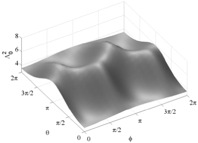
a)b)

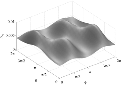
Figure 6: The first and second eigenvalues of the matrix $\mathrm{\mathbf{U}}_{x}^{\mathrm{T}}\mathrm{\mathbf{U}}_{x}$ vs. two angle variable at the boundary of the absorbing area and at $\psi=0$.

Fig. 7 shows values of the function $f$ (16) that it takes on the surface of the absorbing domain at $\chi=1$, $\psi=0$, $\gamma=1.1$ and at the parameters values (12). We see that the function $f$ is always less then $0.5$. The function is smooth and varies sufficiently slow, so that there are no peaks which can be candidates for violation of the inequality (16) between the checked values of $\phi$ and $\theta$. Thus, we can conclude that the inequality (16) is valid.

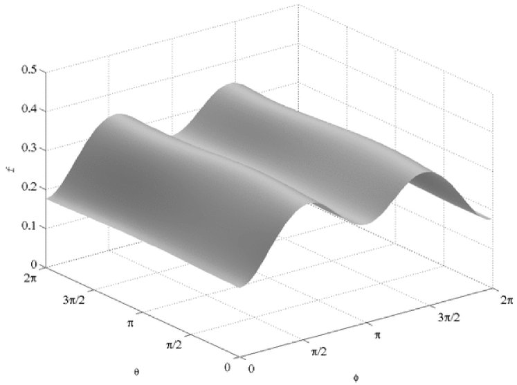
Figure 7: Verification of the inequality (16) on the surface of the absorbing domain at $\psi=0$, $\gamma=1.1$ and at the parameters values (12). Observe, that $f<1$.

a)b)

Figure 8: a) Maximum of $f(\phi,\psi,\theta)$ vs. $\chi$ at $\gamma=1.1$. b) Maximum of $f(\phi,\psi,\theta,\chi)$ vs. $\gamma$. The parameters values are given by (12).

One can see from Fig. 7 that $f$ depends essentially on $\phi$ only, while the dependance on $\theta$ is very weak. The dependance on $\psi$ is tested to be also weak. Plots calculated at different values of $\psi$ looks almost identical to the that shown in Fig. 7. Qualitatively similar plots appear also at $\chi<1$ that corresponds to the interior of the absorbing domain and the inequality (16) remains always valid.

To verify the validity of (16) for the whole absorbing domain, we fix certain value of $\chi$ and find the maximum of $f$ as a function of three angle variables $\phi$, $\psi$, $\theta$. Thus, varying $\chi$, we obtain a function $f_{\mathrm{max}}(\chi)$ that is shown in Fig. 8(a). Notice that the inequality $f_{\mathrm{max}}<1$ is valid both inside the absorbing domain, i.e., at $0\leq\chi\leq 1$, and far beyond.

Now we need to examine the validity of (16) at different $\gamma$. We assume that $f$ is a function of four variables $\phi$, $\psi$, $\theta$ and $\chi$ and find its maximum at each $\gamma$ with additional requirement $0\leq\chi\leq 1$. As follows from Fig. 8(a), $f_{\mathrm{max}}$ grows monotonically vs. $\chi$. Therefore, when a numerical procedure, that seeks a maximum, goes out of the absorbing domain and asks a value of $f$ at $\chi>1$, we return $f$ at $2-\chi$ instead. In fact, we create an artificial maximum at the boundary of the absorbing domain, that prevents the overrun the boundary. If the seeking procedure can not find a maximum in the interior of the absorbing domain, it finds the maximum on the boundary at $\chi=1$. The resulting graph $f_{\mathrm{max}}(\gamma)$ is shown in Fig. 8(b). We see that the inequality $f_{\mathrm{max}}<1$ is definitely fulfilled in a wide range of $\gamma$ both below and above the point $\gamma=1$. This confirms the expected mutual location of expanding and contracting cones in the absorbing domain. Hence, we conclude that the hyperbolicity of the attractor of the system (6) is established. This result can be reproduced for a wide range of values of the parameters of the system (6).

6 Conclusion

In this paper we introduce amplitude equations for a system of two coupled non-autonomous self-oscillators that have uniformly hyperbolic chaotic attractor. We provide an evidence that the system of amplitude equations also demonstrates the hyperbolic chaotic dynamics. Given a certain set of parameters, we find a toroidal absorbing domain that is mapped into itself and contains an attractor of a Poincaré map for this system. Performed computations confirm the validity of sufficient conditions for the hyperbolicity. The conditions are formulated in terms of inclusions of expanding and contracting cones that are defined in a tangent vector space associated with the points of the absorbing domain.

Because of the universality of amplitude equations, the considered system can be a model for dynamics of various physical systems. With this example it is possible to construct other models with hyperbolic chaos, exploiting structural stability of the hyperbolic attractor. A physical experiment demonstrating attractor of this type has been performed already on a basis of coupled electronic oscillators [12]. In applications, the systems with hyperbolic chaos may be of special interest because of their robustness (structural stability). An interesting and now a substantial direction is constructing chains, lattices, networks on a base of elements with hyperbolic chaos [6]. Models of this class may be of interest for understanding deep and fundamental questions, like the problem of turbulence.

This work was partially supported by DFG and RFBR (Grant No. 06-02-16619).

References

- [1] V. S. Afraimovich, V. V. Bykov, L. P. Shilnikov, On the origin and structure of the Lorenz attractor (for dynamic modeling in hydrodynamics and nonlinear optics), Sov. Phys. Dokl. 22 (1977) 253.
- [2] V. S. Afraimovich, S.-B. Hsu, Lectures on chaotic dynamical systems, vol. 28 of AMS/IP Studies in Advanced Mathematics, American Mathematical Society, Providence, RI; International Press, Somerville, MA, 2003.
- [3] V. S. Anishchenko, V. V. Astakhov, A. B. Neiman, T. E. Vadivasova, L. Schimansky-Geier, Nonlinear dynamics of chaotic and stochastic systems. Tutorial and modern development, Springer, Berlin, Heideberg, 2002.
- [4] V. I. Arnol’d, Ordinary defferential equations, Springer-Verlag, 1992.
- [5] G. Benettin, L. Galgani, A. Giorgilli, J. M. Strelcyn, Lyapunov characteristic exponents for smooth dynamical systems and for hamiltonian systems: A method for computing all of them. Part I: Theory. Part II: Numerical application, Meccanica 15 (1980) 9–30.
- [6] L. A. Bunimovich, Y. G. Sinai, Spacetime chaos in coupled map lattices, Nonlinearity 1 (1988) 491.
- [7] R. L. Devaney, An Introduction to Chaotic Dynamical Systems, Addison-Wesley, New York, 1989.
- [8] J.-P. Eckmann, D. Ruelle, Ergodic theory of chaos and strange attractors, Rev. Mod. Phys. 57 (1985) 617.
-
[9]
T. J. Hunt, Low dimensional dynamics: bifurcations of cantori and realisations
of uniform hyperbolicity, Phd thesis, Univ. of Cambridge (2000).
URL http://www.timhunt.me.uk/maths/thesis.ps.gz - [10] A. Katok, B. Hasselblatt, Introduction to the modern theory of dynamical systems, Cambridge University Press, 1995.
- [11] S. P. Kuznetsov, I. R. Sataev, Hyperbolic attractor in a system of coupled non-autonomous van der Pol oscillators: Numerical test for expanding and contracting cones, Phys. Lett. A 365 (2007) 97–104.
- [12] S. P. Kuznetsov, E. P. Seleznev, A strange attractor of the Smale-Williams type in the chaotic dynamics of a physical system, JETP 102 (2006) 355.
- [13] S. P. Kuznetsov, Example of a physical system with a hyperbolic attractor of the Smale-Williams type, Phys. Rev. Lett. 95 (2005) 144101.
- [14] L. D. Landau, E. M. Lifshitz, Fluid mechanics, vol. 6 of Course of Theoretical physics, 2nd ed., Butterworth-Heinemann, 2000.
- [15] L. D. Landau, On the problem of turbulence, Doklady Akademii Nauk SSSR 44 (1944) 339–342, in Russian.
- [16] K. Mischaikow, M. Mrozek, Chaos in the Lorenz equations: A computer-assisted proof, Bull. Am. Math. Soc. 32 (1995) 66.
- [17] E. Ott, Chaos in dynamical systems, Cambridge University Press, 1993.
- [18] T. S. Parker, L. O. Chua, Practical numerical algorithms for chaotic systems, Springer-Verlag, 1989.
- [19] W. H. Press, S. A. Teukolsky, W. T. Vettering, B. P. Flannery, Numerical recipes in C, Cambridge University Press, 1992.
- [20] H. G. Schuster, Deterministic chaos: an introduction, Physik Verlag, Weinheim, 1984.
- [21] L. P. Shilnikov, Mathematical problems of nonlinear dynamics: a tutorial, Int. J. of Bifurcation and Chaos 7 (1997) 1353–2001.
- [22] Y. G. Sinai, Stochasticity of dynamicsl systems, in: A. V. Gaponov-Grekhov (ed.), Nonlinear waves, Nauka, Moscow, 1979, pp. 192–212, in Russian.