The Phoenix Deep Survey: Extremely Red Galaxies and Cluster Candidates

Abstract

We present the results of a study of a sample of 375 Extremely Red Galaxies (ERGs) in the Phoenix Deep Survey, 273 of which constitute a subsample which is 80% complete to $K_{s}=18.5$ over an area of 1160 arcmin². The angular correlation function for ERGs is estimated, and the association of ERGs with faint radio sources explored. We find tentative evidence that ERGs and faint radio sources are associated at $z\gtrsim 0.5$. A new overdensity-mapping algorithm has been used to characterize the ERG distribution, and identify a number of cluster candidates, including a likely cluster containing ERGs at $0.5<z<1$. Our algorithm is also used in an attempt to probe the environments in which faint radio sources and ERGs are associated. We find limited evidence that the $I-K_{s}>4$ criterion is more efficient than $R-K_{s}>5$ at selecting dusty star-forming galaxies, rather than passively evolving ERGs.

1 Introduction

Extremely red objects (EROs) comprise stars, stellar remnants and galaxies. EROs that are not galaxies include brown dwarfs and protostars, and have been studied (e.g. Fan et al., 2000) at infrared $K$ magnitudes $\lesssim$ 15. At fainter magnitudes, most EROs are galaxies. Use of the term “ERO” to describe both classes of objects is widespread, but to avoid confusion, we refer hereafter to the ERO galaxies as extremely red galaxies (ERGs). They have very red colours ($R-K_{s}>5$, $I-K_{s}>4$), and are thought to include members of two distinct populations (e.g. Cimatti, 2003, McCarthy, 2004, Daddi et al., 2004): dusty star-forming galaxies (including some active galactic nuclei, AGNs) and evolved ellipticals at $z\gtrsim 1$. Following the example of Roche et al. (2002), we will refer to the dusty star-forming ERGs as “dsfERGs”, and to the passively evolving ERGs as “pERGs”. The relative mix of the two populations, which is a function of magnitude, colour and redshift, has not been well constrained in the literature, although progress has been made (e.g. Cimatti 2003, Moustakas et al. 2004). The red colours in dsfERGs are caused by dust absorbing shorter wavelength light and in pERGs by old stellar populations.

Different models of galaxy evolution — monolithic collapse with passive luminosity evolution (PLE) versus hierarchical merging in a cold dark matter (CDM) cosmology — predict different properties for galaxy populations. These involve differences in the formation scenario for ellipticals, and in the evolution of the large-scale structure of the universe. The hierarchical merging model predicts that the number of ellipticals should increase with time, as they form through the merging of spiral or irregular systems.

Eisenhardt et al. (2000) found that a high fraction of red galaxies, corresponding to redshifts $z>1$, was at least as consistent with PLE as with CDM merger models. Scodeggio & Silva (2000) found that the space density of ERGs was consistent with no change in the volume density of ellipticals from $z=0$ to 1.5. However, Rodighiero et al. (2001) found evidence for CDM merger models in the form of a decrease in the density of E/S0 galaxies between $z=1$ and 1.5, with a corresponding drop in the density of ERGs. A characteristic limitation of these early ERG surveys was large field-to-field variations in ERG density (e.g. Barger et al. 1999 compared with McCracken et al. 2000). This is largely a result of cosmic variance, but is also related to survey sensitivity and how the ERG class is defined (McCarthy 2004). ERG density is a strong function of both the survey depth and the colour threshold used to define the ERG population.

ERGs include galaxies that formed at high redshift and evolved passively since then (e.g. Firth et al. 2002). For example, Spinrad et al. (1997) studied a pERG at $z=1.55$, estimating that it had a formation redshift $z_{f}\geq 5$ and identifying it as possibly the oldest galaxy known at $z\gtrsim 1$. The detection of highly evolved ellipticals at $1<z<2$ by Benítez et al. (1999), with a corresponding lack of luminous blue ellipticals, also implied a formation redshift for ellipticals of $z_{f}\geq 5$. From ERGs in the K20 survey, Cimatti et al. (2003) deduce a minimum formation redshift of about 2 for pERGs at $z\approx 1$, and a significant range for the formation redshift of about 2.2 to 4.

Even though the evolution of the star-formation rate (SFR) in different environments has not been comprehensively constrained (e.g. Poggianti et al. 2006), it is clear that the lowest SFRs in the nearby universe, found in high mass elliptical galaxies, were the sites of the highest SFRs in the distant past. Smail et al. (1999) suggest that the most extreme ERGs are mainly of the dusty star-forming variety, and that studying the dsfERG population may tell us much about the nature of star formation in the early universe.

Measurement of the densities of pERGs may therefore be used to test models of galaxy evolution in terms of the mass assembly of galaxies, with the clustering properties of both pERGs and dsfERGs being used to test the clustering predictions of these scenarios. The importance of ERGs for such tests is emphasized by Georgakakis et al. (2006), who find that ERGs contribute almost half the stellar mass density of the universe at $z\approx 1$. Furthermore, both ERG classes may provide valuable information about the formation of the earliest galaxies and clusters. Faint radio sources are also considered to identify clusters (e.g. Best 2000, Buttery et al. 2003), but it has not been conclusively shown that ERGs and faint radio sources trace similar structures at high redshift (Georgakakis et al. 2005).

In this paper, we present the results of a moderately deep near-infrared $K_{s}$ survey (Section 2) covering $\approx 1160$ arcmin² in the Phoenix Deep Survey region. Our survey covers a larger area than the $K_{s}$-band survey detailed in Sullivan et al. (2004) but to a shallower depth. Our corresponding ERG sample, defined in Section 3, is about the same numerical size as that studied by Georgakakis et al. (2005, 2006). Our ERG sample is complemented by deep radio data, which we use to examine the association of ERGs and radio sources. Deep multiwavelength coverage allows us to investigate differences in clustering properties which may be introduced by different ERG selection criteria. We examine the environments and clustering of our sample in Sections 4 and 5, focussing on a possible cluster at $0.5<z<1$ in Section 6. Where necessary in this work, we have adopted a concordance cosmological model with $H_{0}=70$ km s^-1 Mpc^-1, $\Omega_{M}=0.3$ and $\Omega_{\Lambda}=0.7$. All magnitudes are in the Vega system.

2 The Phoenix Deep Survey

The Phoenix Deep Survey (PDS) is a multiwavelength survey aimed at studying the nature and evolution of faint radio sources. The radio data, which reaches a minimum $1\,\sigma$ noise level of 12 $\mu$Jy at its most sensitive, defines the survey area of 4.56 deg² in the southern constellation Phoenix. The radio observations (Hopkins et al. 1998, 1999, 2003) were carried out between 1994 and 2001 at the Australia Telescope Compact Array (ATCA).

2.1 Survey Multiwavelength Data Set

Deep multicolour images are available for part of the PDS in $U$, $B$, $V$, $R$ and $I$ bands. BVRI data were obtained in 2001 using the Wide Field Imager (WFI) at the Anglo-Australian Telescope (AAT), Siding Spring Observatory. $U$ band data were collected at the Cerro Tololo Inter-American Observatory (CTIO) in 2003, while deep near-infrared data ($K_{s}\lesssim 20$) are acquired for a 180 arcmin² region using the Son of ISAAC (SofI) instrument at the European Southern Observatory’s (ESO) New Technology Telescope (NTT) at La Silla. Details of the optical and near-infrared observations are given in Sullivan et al. (2004). The $R-$ and $I-$ band catalogs have 5 $\sigma$ limiting magnitudes of 24.61 and 24.67 respectively, using SExtractor’s (Bertin & Arnouts 1996) MAG_AUTO photometry.

2.2 Extended Near-Infrared Dataset

In addition to the SofI data, near-infrared images ($K_{s}\lesssim$ 18.5) covering an area of 1160 arcmin² of the PDS were obtained with the Infrared Side Port Imager (ISPI) camera at CTIO on 2004 September 25. The conditions were photometric, with seeing ranging from $0\farcs 8$ to $1\farcs 2$. We observed 11 ISPI pointings using a random dither pattern, nine with a total exposure time of 30 minutes, and the remaining two with exposure times of 21 and 15 minutes. Image processing was performed using standard NOAO IRAF routines. Dark frames were subtracted from each image, as were running sky flats, constructed from medians of up to 10 object frames. The IRAF tasks mscgetcat and msccmatch were used to accurately register the images for co-addition. The final astrometry was done by reference to 2MASS (Skrutskie et al. 2006) source positions. Residual offsets with respect to 2MASS positions, and to fainter PDS sources in $R$-band images, were fitted by a Gaussian with $\sigma=0\farcs 3$.

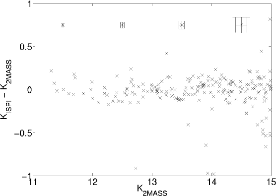
Figure 1: A comparison of the 2MASS and ISPI magnitudes after photometric calibration, for objects with $K_{s}<15$. The points significantly below the line arise from extended or saturated objects, resulting in erroneous integrated fluxes. The error boxes indicate the typical uncertainties as a function of magnitude.

We employed SExtractor on each of the eleven $K_{s}$-band images using their respective exposure maps as weight images, with a detection threshold of 1.5 times the noise level. The low signal-to-noise regions on the edges of the co-added images, a result of the dithering of individual exposures, are excluded with simple right ascension and declination cuts. The overlap between the images was such that we were able to maintain contiguity throughout the area of our $K_{s}$-band survey. The final catalogue contains 4834 objects. Within the area of our catalogue, there are 230 sources, mostly stars, which also have 2MASS identifications. For each individual image, we tied our photometry to 2MASS by adjusting the magnitude zeropoints in our SExtractor input to give the tightest correlation between ISPI and 2MASS magnitudes (see Figure 1).

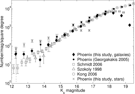
Figure 2: Differential galaxy source counts, compared with counts from Georgakakis et al. (2005), Schmidt et al. (2006), Szokoly et al. (1998) and Kong et al. (2006). Differential star counts are also shown. The large error bar for the Georgakakis et al. point at $K_{s}=12.25$ arises from a single object in that bin. The high counts at the bright end of our sample may arise from a small systematic overestimation of brightness by SExtractor at these levels.

Following Schmidt et al. (2006), we performed star-galaxy separation by comparing SExtractor’s fixed aperture ($3\farcs 5$ diameter) magnitude with its MAG_AUTO magnitude, after which we used MAG_AUTO for all subsequent analysis. Our $K_{s}$-band galaxy counts shown in Figure 2 are consistent with other recent measurements. The completeness of the catalogue was estimated to be 80% to $K_{s}=18.5$ from comparison with source counts from Kong et al. (2006).

3 The ERG Sample

3.1 ERG Selection

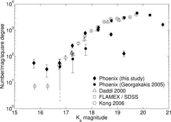
Figure 3: Differential ERG number counts for the $R-K_{s}>5$-selected sample compared with Georgakakis et al. (2005), Daddi et al. (2000), FLAMEX/SDSS (Elston et al. 2006) and Kong et al. (2006). Our counts at the bright end are subject to small number statistics.

We matched our near-infrared catalogue with the existing optical catalogue (Sullivan et al. 2004), counting objects within 2^′′ as matches. We constructed two samples of ERGs based on the two-colour criteria: $R-K_{s}>5$ and $I-K_{s}>4$. This resulted in a sample of 375 $R-K_{s}$-selected ERGs, 273 of which are brighter than $K_{s}=18.5$. Similarly, we derived a sample of 346 $I-K_{s}$-selected ERGs, 256 of which are brighter than $K_{s}=$18.5. 301 ERGs are common to both samples, 228 of which are brighter than $K_{s}=$18.5. Figure 3 shows a comparison of the differential $R-K_{s}$ ERG counts with those from previous studies. ERGs with more extreme colours close to the $K_{s}$-band detection limit may not be detected in $R$-band, and will therefore contribute to the incompleteness seen in Figure 3.

3.2 ERG Correlation Function

To characterize the clustering properties of this ERG sample, we use the two-point angular correlation function. We follow the prescription detailed by Georgakakis et al. (2005), using the Landy & Szalay (1993) estimator for calculating $w(\theta)$, with uncertainties that are assumed to be Poissonian. We also apply an integral constraint ($C$), again as detailed by Georgakakis et al. (2005), assuming the correlation function slope $\delta=0.8$, which gives $C=5.42$ for our survey area.

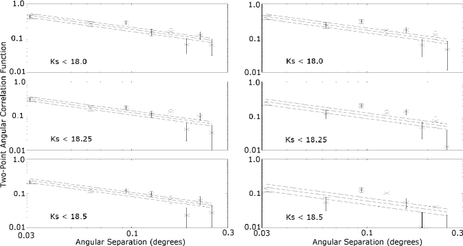
Figure 4: Correlation functions for the ERG samples as a function of limiting magnitude. Left: $R-K_{s}>5$ and Right: $I-K_{s}>4$. The value of $\delta$ is fixed at 0.8 and the upper and lower lines signify $\pm 1\,\sigma$ uncertainties. The increased scatter in the $I-K_{s}$-selected samples, introduced by a small number of objects that are not common to both samples, illustrates the difference between the clustering properties of the ERG samples selected by the two criteria.

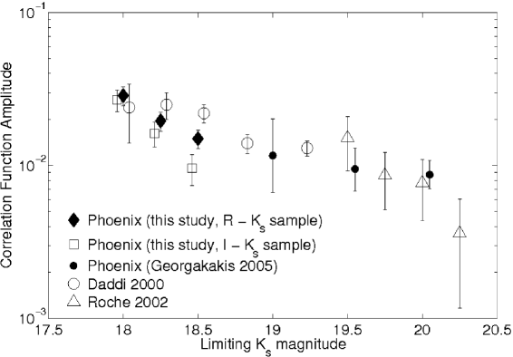
Figure 5: Clustering amplitudes for the $R-K_{s}>5$ and $I-K_{s}>4$ samples compared with those found by Georgakakis et al. (2005), Daddi et al. (2000) and Roche et al. (2002). For clarity, points at the same limiting magnitude have been offset horizontally by $\pm 0.04$ mag. At a limiting magnitude of $K_{s}=18.5$ our clustering amplitudes are significantly lower than Daddi et al. because of our survey incompleteness.

In Figure 4 we present the correlation functions for the ERGs from our data. We find significant clustering for limiting $K_{s}$ magnitudes between 18 and 18.5 (Table 1). The clustering amplitudes for our ERG sample are consistent with other recent measurements (Figure 5), and are much greater than the amplitudes which have been measured for all $K_{s}$-band galaxies to the same limiting magnitudes (e.g. Daddi et al., 2000). There appears to be a difference between the clustering properties of the ERGs selected by our two different criteria. In Table 1, at each limiting magnitude, the clustering amplitude and confidence level of the clustering signal for ERGs selected using the $R-K_{s}$ criterion is greater than that found using $I-K_{s}$ selection. This is also seen in Figure 4, supporting the suggestion (Väisänen & Johansson 2004) that $I-K_{s}$ selection may be more sensitive to the dsfERG population, as these galaxies are expected to cluster less strongly than the pERGs. We stress that differences in the redshift distributions of ERGs selected by the different colour criteria are likely to affect their measured clustering properties. Observed-frame colour tracks given by McCarthy (2004) show that the $R-K_{s}$ criterion should, in principle, be more efficient at selecting passively evolving ERGs.

4 ERG Environments

Studying the association of ERGs with $K_{s}$-band galaxies and faint radio sources is valuable in understanding their nature. For this analysis we have used the ERG sample selected with $R-K_{s}>5$.

Our estimation of the cross-correlation between $K_{s}$-band galaxies and ERGs reveals no significant association. Given the depth of our survey, in which most of the $K_{s}$-band galaxies lie at $z\ll 1$, this is not unexpected, since ERGs are found predominantly at $z\approx 1$. Georgakakis et al. (2005) find that ERGs are only associated with overdensities of $K_{s}$-band galaxies at $z\gtrsim 1$.

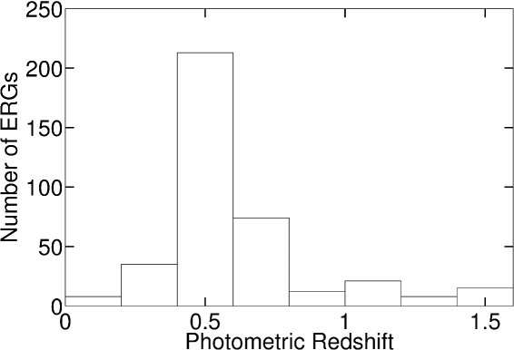
Figure 6: Photometric redshift distribution for the $R-K_{s}>5$ ERG sample.

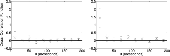
Figure 7: Cross-correlation functions with bootstrap errors for ERGs around faint radio sources with optical counterparts assigned photometric redshifts (not shown in Figure 6). Left: 97 radio sources associated with galaxies at $z_{\rm phot}<0.4$ and Right: 98 sources with $z_{\rm phot}>0.5$. As discussed, our exclusion of faint radio sources individually associated with ERGs ensures that the small-scale feature is not the result of one-to-one associations.

To compare the ERG and faint radio source populations, we first make use of the publicly available code hyperz (Bolzonella et al. 2000) to find photometric redshifts for all galaxies detected in at least three of the UBVRIK_s bands. In Figure 6 we have shown the photometric redshift distribution for $R-K_{s}$ ERGs only. We then match our radio catalogue with the galaxies (including non-ERGs) for which we have photometric redshifts, dividing the radio sources into two broad redshift ranges. Faint radio sources individually associated with ERGs are excluded, and cross-correlation functions are estimated (e.g. Georgakakis et al. 2005) to compare the two radio samples with the ERG catalogue. Figure 7, in which bootstrap errors are shown (Barrow, Bhavsar & Sonoda 1984), demonstrates that while there is no significant correlation between the positions of ERGs and faint radio sources with counterparts at $z_{\rm phot}<0.4$, there is such a correlation at the $2.3\,\sigma$ confidence level for the radio sources with counterparts at $z_{\rm phot}>0.5$. Georgakakis et al. (2005) also detect such a correlation at the $\approx 2\,\sigma$ confidence level.

Our work supports the conclusion that at higher redshifts ($z\gtrsim 0.5$), ERGs and radio sources are associated. This is perhaps not surprising since the redshift distributions of both samples peak at $z\approx 1$ (Condon 1989, McCarthy 2004). Since we have eliminated faint radio sources individually associated with ERGs, this cannot simply be the result of one-to-one associations. If ERGs and radio sources trace galaxy overdensities at higher redshift, we should be able to detect strong association between the two populations in high redshift cluster environments. In the next section we search for this effect.

5 Cluster Candidates

Rich clusters at high redshifts contain massive, red elliptical galaxies at their cores, which can show up as ERG overdensities a few arcminutes across in ERG surveys (e.g. Stanford et al. 1997, Roche et al. 2002, Díaz-Sánchez et al. 2007). Studies of such cluster samples may be used to investigate how the highest density regions of the universe have evolved, and possibly place constraints on their formation.

Here we identify cluster candidates in two different ways. First, we use a simple counts-in-cells criterion, and second, we use an overdensity-mapping algorithm. The former technique gives us a set of likely candidates, and the latter technique allows us to treat cluster environments statistically.

5.1 Counts-In-Cells

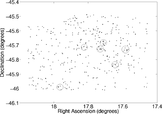
Figure 8: Our ERG field showing the circled locations of the cluster candidates based on our counts-in-cells criterion (see section 5.1). The cross indicates the probable $0.5<z<1$ cluster discussed in section 6.

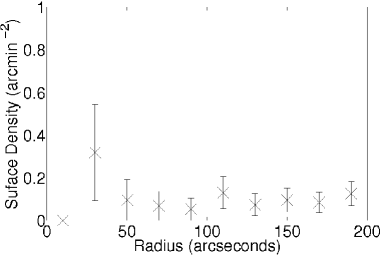
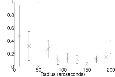
Figure 9: Density profiles for faint radio sources around the six positions (see Figure 8) which lie at the centres of overdensities selected via the counts-in-cells criterion. Left: $z_{\rm phot}<0.4$ radio sources, and Right: $z_{\rm phot}>0.5$ sources. For this measurement we have not eliminated objects that are both ERGs and faint radio sources. The horizontal lines in each panel correspond to the average radio source density.

For the entire area of our survey we have found local counts of ERGs within circles of radius 50 arcseconds, and identified six locations (Figure 8) which contain six or more ERGs within a circle of radius 50 arcseconds (see also Blake & Wall 2002). Given a uniform random field with the same mean density as our ERG catalogue, the probability of a particular location hosting such an overdensity is 3.8 $\times$ 10^-4. This criterion selects locations hosting the highest densities and is intended to identify overdensities with the highest probability of physical significance. Díaz-Sánchez et al. (2007) report one such overdensity as a cluster at $z\approx 1$. Figure 9 shows the distribution of faint radio sources in these cluster environments, for the same redshift ranges used in Figure 7. One might expect from the statistically significant result for $z>0.5$ in Figure 7 that there should also be an excess of associated radio sources in the regions with ERG overdensities. However, we find only a 1.05 $\sigma$ excess of faint radio sources in these putative clusters. This may be because the ERGs in these high density regions are pERGs which have fewer radio counterparts since they have lower star-formation rates.

5.2 Overdensity-Mapping Algorithm

We now describe an algorithm we have developed to identify overdensities of ERGs within our survey area, beginning with a general description before explaining the procedure in detail. For any given location, we compare the local galaxy count with the distribution of counts expected from a large set of uniform random catalogues, each with the same mean density as the ERG catalogue. This comparison allows us to calculate the probability that the local area contains a greater number of galaxies than that expected from a random distribution. Repeating this process for a range of specific radii, we form a probability function which is then associated with the location. Similarly, a probability function is assigned to each of a set of uniformly spaced locations within our survey. The optimal range and resolution of the radii and locations sampled may be found empirically.

Each probability function is used to estimate the probability of the count within each radius enclosing its location occurring as the result of a uniform random distribution. If the probability of obtaining the local count from a random catalogue is high, the value of the probability function will be close to a half, since the number of random catalogues with lower counts will be similar to the number with higher counts. In the presence of a genuine overdensity, the probability function will rise above 0.5 and continue to ascend with increasing radius (since the probability of a large overdensity is lower than the probability of a small one) until the “edge” of the overdensity has been reached. Beyond this edge, the enclosed density will fall back to the background density, and the probability function will approach 0.5. Hence, we expect each probability function to be sensitive to both the significance and scale of any nearby overdensities, characterised by its maximum and the radius at which it occurs.

For overdensities centred on particular catalogue objects, this maximum occurs at a radius of zero (which thus encloses an infinite density), but we negate this by specifying a minimum overdensity membership of two. We define the radius at which the maximum occurs as the overdensity radius, and the overdensity probability as the value which the probability function takes at the overdensity radius. Our technique uses probability to compare between scales in order to select the most likely scale at which each particular location hosts an overdensity.

To achieve this, we follow these steps.

• The survey area is covered with a uniform grid of test points at intervals of 20 arcseconds along both right ascension and declination.

• We populate the survey area with a large number of random sets, each containing the same average density of points as the ERG catalogue that we are examining.

• We count the number of ERGs and random objects (in each random set) as a function of distance from each test point, in steps of 10 arcseconds from 20 to 120 arcseconds.

• The probability of overdensity is then the fraction of random sets for which the number of ERG counts exceeds the number of random counts. ERG counts consistent with uniform random distribution will therefore produce overdensity probabilities of 0.5.

In overdense regions, the overdensity probability directly quantifies the probability that the local environment is associated with an overdensity, and the overdensity radius directly characterizes the scale size of this structure. Each of the grid points which we test within our catalogue will have an associated overdensity probability and overdensity radius. By confining our random sets to the area of the catalogue under inspection, we account for edge effects.

The probability of overdensity is intimately connected with the overdensity radius. We are effectively sensitive to multi-scale structure throughout the survey area, meaning that we will detect both high density small-scale features (which might be overlooked in the case of simple large-scale smoothing), and extended regions of intermediate density (which might be overlooked in the case of simple small-scale smoothing). Our algorithm is therefore sensitive to overdensities spanning a wide range of scales. In particular it has the potential to simultaneously identify filamentary structures as well as clusters, an aspect that we will explore in detail in future work.

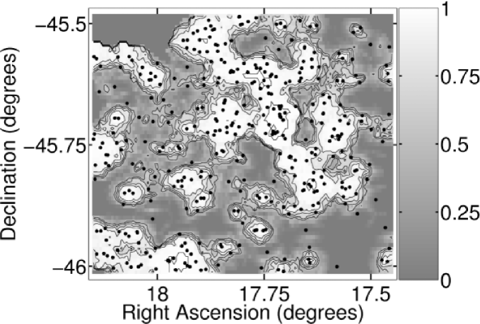
Figure 10: Grayscale representation of our overdensity probability map for the $R-K_{s}$-selected ERG sample (see section 5.2). The black dots are the ERGs in this sample and the contours correspond to probabilities of 0.5, 0.625, 0.75, 0.875 and 1. There is clear evidence of filamentary structure in the high density islands.

Figure 10 shows the result of the overdensity-mapping algorithm applied to our data. It is clear that the regions identified by our algorithm as having a high overdensity probability do indeed correspond to visual overdensities of ERGs, and similarly that regions with no ERGs, or isolated ERGs, have low probability.

5.3 Faint Radio Sources and the Overdensity Map

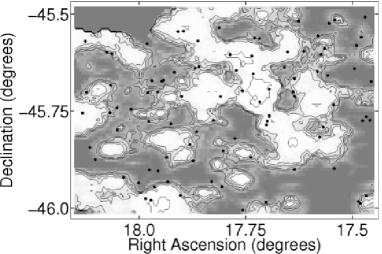
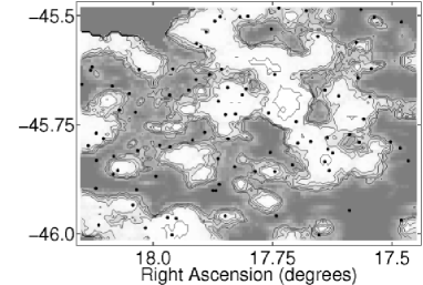
Figure 11: Grayscale as in Figure 10, with black dots indicating the locations of faint radio sources. Left: 97 sources with $z_{\rm phot}<0.4$. Right: 98 sources with $z_{\rm phot}>0.5$.

In Figure 11 we visually compare the overdensity probability map in Figure 10 with the distribution of faint radio sources in the two $z_{\rm phot}$ ranges previously defined. The redshift dependence shown in Figure 7 is not apparent in Figure 11. We stress, however, that since our algorithm has smoothed the predominantly $z\approx 1$ ERG population, the overdensity map will be biased towards structures at this redshift.

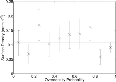
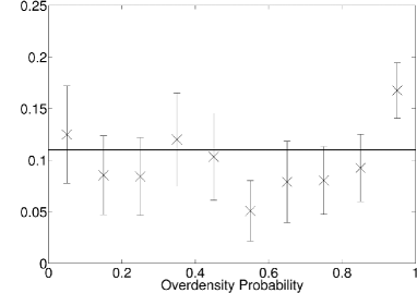
Figure 12: Surface density of radio sources as a function of overdensity probability. Left: Sources with $z_{\rm phot}<0.4$. Right: Sources with $z_{\rm phot}>0.5$. The error bars are Poissonian and the horizontal lines correspond to the average source density.

We have matched each of the faint radio sources with the pixel (from our overdensity map) closest to its position, and counted the frequency with which faint radio sources are matched with certain pixel values. Effectively, what we are doing here is counting the number of faint radio sources which lie along different probability contours of our overdensity map. The result of this analysis is shown in Figure 12, which suggests that faint radio sources with optical counterparts with $z_{\rm phot}>0.5$ are indeed found in high density regions, with a 2$\sigma$ excess for overdensity probabilities between 0.9 and 1. This is not seen in the $z_{\rm phot}<0.4$ sample. While the statistics are poor, and our overdensity map is strongly biased towards higher redshifts (as shown in Figure 6), Figure 12 tentatively suggests that clusters at high redshift are more likely to host faint radio sources in their central regions.

The lack of a clear association of ERGs and radio sources with optical counterparts with $z_{\rm phot}>0.5$ evident in Figure 11 and the result from Figure 9 suggests that the correlation between ERGs and moderately high redshift radio sources implied by Figure 7 does not occur in regions with the highest ERG densities. Figure 7 shows association on scales which may not be noticeable when considering the scale of the entire field shown in Figure 11, and cannot be used to draw conclusions about the characteristic density of the environment in which ERGs and faint radio sources are associated. Figure 12 illustrates, however, that our overdensity map provides a way of directly probing this characteristic density.

6 A Possible Cluster at $0.5<z<1$

Of the cluster candidates identified via the counts-in-cells criterion (Figure 8), we have singled out one in particular as an interesting object for future study.

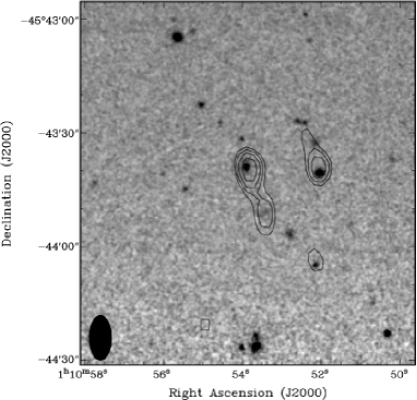
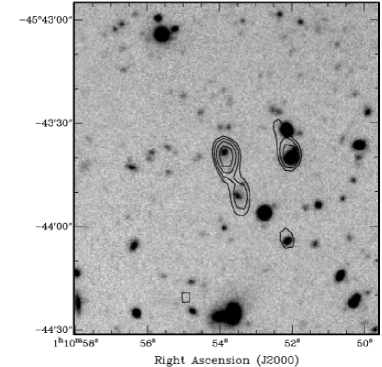
Figure 13: Images of a possible $0.5<z<1$ cluster (see Section 6). Left: $K_{s}$-band; Right: $R$-band. Overlaid contours at 1.4 GHz from the Phoenix Deep Survey are at 36, 47, 61 and 79 $\mu$Jy/beam. The ATCA synthesised beam (12${}^{\prime\prime}\times 6^{\prime\prime}$ in position angle 0^∘) is shown in the lower left hand corner of the $K_{s}$-band image.

$K_{s}$-band and $R$-band images of this putative cluster are shown in Figure 13, with ATCA 1.4 GHz contours overlaid. Astrometry for both images was referenced to 8–10 stars in the SuperCOSMOS (Hambly et al. 2001) $R$-band image which has formal fit errors of 0.11 arcsec rms in each coordinate. The bright ($K_{s}=16.3$) central radio source PDF J011053.8$-$454339 has a flux density of $S_{1.4}=$ $106\,\mu$Jy. At this flux density, the relative proportions of starburst galaxies and AGNs in the faint radio population are strongly model dependent (e.g. Seymour et al. 2004, Hopkins 2004), although recent observations (Seymour et al. 2008) indicate that star-forming galaxies at this flux density are more numerous than AGNs by a factor of 2 to 3. Figure 13 shows that the central radio source has a nearby companion radio source, PDF J011053.4$-$454351, associated with a faint $K_{s}$-band object that falls below our catalogue threshold.

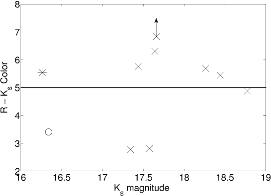
Figure 14: Colour-magnitude diagram for the galaxies in the probable $0.5<z<1$ cluster (Figures 8 and 13) within $22^{\prime\prime}$ of the brightest galaxy. The brightest galaxy is marked with an asterisk, and the western tailed radio source host is marked with a circle.

Figure 14 shows there are six objects in this possible cluster with $R-K_{s}\geq 5.4$. Since such extreme colours are caused primarily by redshift, the cluster is likely to lie at $0.5<z<1$ but not much greater, given the depth of our $K_{s}$ survey. If it lies at $z=1$, the radio luminosity of the central ERG is $L_{1.4}=5\times 10^{23}\,$W Hz^-1, making it a low-luminosity AGN. As the brightest galaxy in this field, it is also consistent with being the central dominant cluster galaxy.

An 80 $\mu$Jy radio source to the west (PDF J011052.0$-$454338) is also shown in Figure 13, with contours suggestive of a head-tail morphology. Tailed radio galaxies are often seen in galaxy clusters (e.g. Gomez et al. 1997, Sakelliou & Merrifield 2000, Klamer et al. 2004), but its $R=20.4$ magnitude and clear separation from the red locus in Figure 14 point to it belonging to the foreground cluster evident in the $R$-band image.

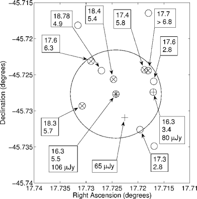
Figure 15: The vicinity of the probable $0.5<z<1$ cluster, showing the locations of cataloged $K_{s}$-band galaxies ($\bigcirc$), faint radio sources ($+$) and ERGs ($\times$). Where available, we have labeled each object with $K_{s}$ magnitude, $R-K_{s}$ colour and radio flux density. A circle of radius 22 arcseconds is also shown.

Figure 15 shows that the ERGs associated with this overdensity all fall within 22 arcseconds of the central ERG, corresponding to a projected radius of $\sim$0.18 Mpc at $z\approx 1$. This is less than 1/5 of an Abell radius (e.g. Abell 1965). However, the radial extent of the cluster is likely to be underestimated because of our relatively bright $K_{s}$-band limiting magnitude. The presence of radio sources within our empirically determined radial extent suggests that this estimate is consistent with the core radius of 167 kpc found for nearby clusters, based on their radio source distribution (Ledlow & Owen 1995).

7 Summary and Future Work

Within the Phoenix Deep Survey we have identified a sample of ERGs over a large area (1160 arcmin²) that is 80% complete to a limiting magnitude of $K_{s}=18.5$. The number counts and clustering properties of our ERG sample are consistent with previous observations. Based on photometric redshifts we find evidence for the association of ERGs and faint radio sources with $z_{\rm phot}>0.5$, but not with $z_{\rm phot}<0.4$, consistent with earlier results on the evolution of star formation and AGN activity.

We find weak evidence to suggest that $R-K_{s}$-selected ERGs are more strongly clustered than $I-K_{s}$-selected ERGs. If confirmed with more extensive datasets, this would imply that $R-K_{s}$-selected ERGs are more strongly associated with overdensities, supporting the suggestion by Väisänen & Johansson (2004) that $R-K_{s}$-selected ERGs contain a higher proportion of passively evolving sources, assuming that the two ERG populations have similar redshift distributions.

The identification of the cluster candidates in this study shows that ERGs can be used to identify overdensities of potential physical significance, and our 2.3 $\sigma$ result for the association of ERGs and faint radio sources at $z_{\rm phot}>0.5$ is evidence that both classes of objects trace overdense regions. As passive galaxies dominate in high density environments, the absence of radio source overdensities in most of our cluster candidates supports the results of Georgakakis et al. (2006) and Simpson et al. (2006) that dsfERGs are more closely associated with the radio population than pERGs. As a result, faint radio sources are most efficient at identifying starburst galaxies in the infall regions of clusters. The probable $0.5<z<1$ cluster identified here will be explored in more detail with spectra and deeper imaging.

We have introduced a method for quantifying overdensities in a galaxy distribution that is sensitive to overdensities on a broad range of scales, and demonstrated its efficiency in identifying cluster candidates. A faster implementation of this algorithm is being developed.

ERG sample size is a strong function of limiting $K_{s}$-band magnitude, and it is necessary to have complementary deep optical $R$- and $I$-band data to detect ERGs with the most extreme colours. Large samples of ERGs are becoming available with the next generation of large area near-infrared surveys, such as UKIDSS (Lawrence et al. 2007). Where these overlap with existing deep radio surveys, it will be possible to explore the association of the faint radio population with ERGs in unprecedented detail.

Table 1: Correlation Function Amplitudes $A$

		$K_{s}$ limiting magnitude
Selection	Properties	18.0	18.25	18.5
$R-K_{s}$	$A$ ($\times 10^{-3}$)	$28.7\pm 4.1$	$19.6\pm 2.8$	$15.0\pm 2.1$
	$N$	143	202	273
$I-K_{s}$	$A$ ($\times 10^{-3}$)	$26.9\pm 4.4$	$16.2\pm 3.0$	$9.6\pm 2.2$
	$N$	132	188	256

References

- Abell (1965) Abell, G.O. 1965, ARA&A, 3, 1
- Barger et al. (1999) Barger, A.J., Cowie, L.L., Trentham, N., Fulton, E., Hu, E.M., Songaila, A. & Hall, D. 1999, AJ, 117, 102
- Barrow, Bhavsar & Sonoda (1984) Barrow, J.D., Bhavsar, S.P. & Sonoda, D.H. 1984, MNRAS, 210, 19P
- Benítez et al. (1999) Benítez, N., Broadhurst, T., Bouwens, R., Silk, J. & Rosati, P. 1999, ApJ, 515L, 65
- Bertin & Arnouts (1996) Bertin, E. & Arnouts, S. 1996, A&AS, 117, 393
- Best (2000) Best, P.N. 2000, MNRAS, 317, 720
- Blake & Wall (2002) Blake, C. & Wall, J. 2002, MNRAS, 337, 993
- Bolzonella et al. (2000) Bolzonella, M., Miralles, J.-M. & Pelló, R. 2000, A&A, 363, 476
- Buttery et al. (2003) Buttery, H.J., Cotter, G., Hunstead, R.W. & Sadler, E.M. 2003, New Astron Rev, 47, 329
- Cimatti (2003) Cimatti, A. 2003, Revista Mexicana de Astronomia y Astrofisica Conference Series, 17, 209
- Condon (1989) Condon, J.J. 1989, ApJ, 338, 13
- Daddi et al. (2000) Daddi, E., Cimatti, A., Pozzetti, L., Hoekstra, H., Röttgering, H.J.A., Renzini, A., Zamorani, G. & Mannucci, F. 2000, A&A, 361, 535
- Daddi et al. (2004) Daddi, E., Cimatti, A., Renzini, A., Fontana, A., Mignoli, M., Pozzetti, L., Tozzi, P. & Zamorani, G. 2004, ApJ, 617, 746
- Díaz-Sánchez et al. (2007) Díaz-Sánchez, A., Villo-Pérez, I., Pérez-Garrido, A. & Rebolo, R. 2007, MNRAS, 377, 516
- Eisenhardt et al. (2000) Eisenhardt, P., Elston, R., Stanford, S.A., Dickinson, M., Spinrad, H., Stern, D. & Dey, A. 2000, ArXiv Astrophysics e-prints, astro-ph/0002468
- Elston et al. (2006) Elston, R.J., Gonzalez, A.H., McKenzie, E., Brodwin, M., Brown, M.J.I., Cardona, G., Dey, A., Dickinson, M., Eisenhardt, P.R., Jannuzi, B.T., Lin, Y.-T., Mohr, J.J., Raines, S.N., Stanford, S.A., Stern, D. 2006, ApJ, 639, 816
- Fan et al. (2000) Fan, X., Knapp, G.R., Strauss, M.A. et al., 2000, AJ, 119, 928
- Firth et al. (2002) Firth, A.E., Somerville, R.S., McMahon, R.G. et al., 2002, MNRAS, 332, 617
- Georgakakis et al. (2005) Georgakakis, A., Afonso, J., Hopkins, A.M., Sullivan, M., Mobasher, B. & Cram, L.E. 2005, ApJ, 620, 584
- Georgakakis et al. (2006) Georgakakis, A., Hopkins, A.M., Afonso, J., Sullivan, M., Mobasher, B. & Cram, L.E. 2006, MNRAS, 367, 331
- Gomez et al. (1997) Gomez, P.L., Pinkney, J., Burns, J.O., Wang, Q., Owen, F.N. & Voges, W. 1997, ApJ, 474, 580
- Hambly et al. (2001) Hambly, N.C., MacGillivray, H.T., Read, M.A., Tritton, S.B., Thomson, E.B., Kelly, B.D., Morgan, D.H., Smith, R.E., Driver, S.P., Williamson, J., Parker, Q.A., Hawkins, M.R.S., Williams, P.M. & Lawrence, A. 2001, MNRAS, 326, 1279
- Hopkins at al. (1998) Hopkins, A.M., Mobasher, B., Cram, L. & Rowan-Robinson, M. 1998, MNRAS, 296, 839
- Hopkins et al. (1999) Hopkins, A., Afonso, J., Cram, L. & Mobasher, B. 1999, ApJ, 519L, 59
- Hopkins et al. (2003) Hopkins, A.M., Afonso, J., Chan, B., Cram, L.E., Georgakakis, A. & Mobasher, B. 2003, AJ, 125, 465
- Hopkins (2004) Hopkins, A.M. 2004, ApJ, 615, 209
- Klamer et al. (2004) Klamer, I., Subrahmanyan, R. & Hunstead, R.W. 2004, MNRAS, 351, 101
- Kong et al. (2006) Kong, X., Daddi, E., Arimoto, N., Renzini, A., Broadhurst, T., Cimatti, A., Ikuta, C., Ohta, K., da Costa, L., Olsen, L.F., Onodera, M. & Tamura, N. 2006, ApJ, 638, 72
- Landy & Szalay (1993) Landy, S.D. & Szalay, A.S. 1993, ApJ, 412, 64
- Lawrence et al. (2007) Lawrence, A., Warren, S.J., Almaini, O., Edge, A.C., Hambly, N.C., Jameson, R.F., Lucas, P., Casali, M., Adamson, A., Dye, S., Emerson, J.P., Foucaud, S., Hewett, P., Hirst, P., Hodgkin, S.T., Irwin, M.J., Lodieu, N., McMahon, R.G., Simpson, C., Smail, I., Mortlock, D. & Folger, M. 2007, MNRAS, 379, 1599
- Ledlow & Owen (1995) Ledlow, M.J. & Owen, F.N. 1995, AJ, 109, 853
- McCarthy (2004) McCarthy, P.J. 2004, ARA&A, 42, 477
- McCracken et al. (2000) McCracken, H.J., Metcalfe, N., Shanks, T., Campos, A., Gardner, J.P. & Fong, R. 2000, MNRAS, 311, 707
- Moustakas et al. (2004) Moustakas, L.A., Casertano, S., Conselice, C.J., Dickinson, M.E., Eisenhardt, P., Ferguson, H.C., Giavalisco, M., Grogin, N.A., Koekemoer, A.M., Lucas, R.A., Mobasher, B., Papovich, C., Renzini, A., Somerville, R.S. & Stern, D. 2004, ApJ, 600, L131
- Poggianti et al. (2006) Poggianti, B.M., von der Linden, A. & De Lucia, G. 2006, ApJ, 642, 188
- Roche et al. (2002) Roche, N.D., Almaini, O., Dunlop, J., Ivison, R.J. & Willott, C.J. 2002, MNRAS, 337, 1282
- Rodighiero et al. (2001) Rodighiero, G., Franceschini, A. & Fasano, G. 2001, MNRAS, 324, 491
- Sakelliou & Merrifield (2000) Sakelliou, I. & Merrifield, M.R. 2000, MNRAS, 311, 649
- Schmidt et al. (2006) Schmidt, S.J., Connolly, A.J. & Hopkins, A.M. 2006, ApJ, 649, 63
- Scodeggio & Silva (2000) Scodeggio, M. & Silva, D.R. 2000, A&A, 359, 953
- Seymour et al. (2004) Seymour, N., McHardy, I.M. & Gunn, K.F. 2004, MNRAS, 352, 131
- Seymour et al. (2008) Seymour, N., Dwelly, T., Moss, D., McHardy, I., Zoghbi, A., Rieke, G., Page, M., Hopkins, A. & Loaring, N. 2008, MNRAS, (in press; arxiv:0802.4105).
- Simpson et al. (2006) Simpson, C., Almaini, O., Cirasuolo, M., Dunlop, J., Foucaud, S., Hirst, P., Ivison, R., Page, M., Rawlings, S., Sekiguchi, K., Smail, I. & Watson, M. 2006, MNRAS, 373, L21
- Smail et al. (1999) Smail, I., Ivison, R.J., Kneib, J.P., Cowie, L.L., Blain, A.W., Barger, A.J., Owen, F.N. & Morrison, G. 1999, MNRAS, 308, 1061
- Spinrad et al. (1997) Spinrad, H., Dey, A., Stern, D., Dunlop, J., Peacock, J., Jimenez, R. & Windhorst, R. 1997, ApJ, 484, 581
- Stanford et al. (1997) Stanford, S.A., Elston, R., Eisenhardt, P.R., Spinrad, H., Stern, D. & Dey A. 1997, AJ, 114, 2232
- Skrutskie et al. (2006) Skrutskie, M.F., et al. 2006, AJ, 131, 1163
- Sullivan et al. (2004) Sullivan, M., Hopkins, A.M., Afonso, J., Georgakakis, A., Chan, B., Cram, L.E., Mobasher, B. & Almeida, C. 2004, ApJS, 155, 1
- Szokoly et al. (1998) Szokoly, G.P., Subbarao, M.U., Connolly, A.J. & Mobasher, B. 1998, ApJ, 492, 452
- Väisänen & Johansson (2004) Väisänen, P. & Johansson, P.H. 2004, A&A, 422, 453