INSTITUT NATIONAL DE RECHERCHE EN INFORMATIQUE ET EN AUTOMATIQUE

True amplitude one-way propagation in heterogeneous media
Hélène Barucq — Bertrand Duquet — Frank Prat N° ????
Avril 2008

Abstract: This paper deals with the numerical analysis of two one-way systems derived from the general complete modeling proposed by M.V. De Hoop. The main goal of this work is to compare two different formulations in which a correcting term allows to improve the amplitude of the numerical solution. It comes out that even if the two systems are equivalent from a theoretical point of view, nothing of the kind is as far as the numerical simulation is concerned. Herein a numerical analysis is performed to show that as long as the propagation medium is smooth, both the models are equivalent but it is no more the case when the medium is associated to a quite strongly discontinuous velocity.

Key-words: Microlocal numerical analysis, one-way formulation, acoustic waves

Propagation one-way à amplitude prśervée dans des milieux hétérogènes

Résumé : Dans ce travail, on s’int鲥sse à deux formulations one-way de l’équation des ondes acoustique qui ont été construites à partir du modèle complet one-way proposé par M.V. De Hoop. Le principal objectif de cette étude est de comparer les deux formulations dans lesquelles on a introduit un terme permettant d’améliorer le calcul de l’amplitude de la solution numérique. Il ressort de l’analyse que même si les deux systèmes sont équivalents du point de vue théorique, il n’en est rien au niveau des performances numériques. On montre en particulier que tant que le milieu de propagation est régulier, les deux modèles se comportent identiquement et que les différences sont nettes si le milieu comporte des hétérogéités. On peut donc en conclure que le précision de l’amplitude est très sensible à la formulation du modèle.

Mots-clés : Analyse micro-locale numérique, formulation one-way, ondes acoustiques

1 Introduction

The numerical solution of seismic acoustic waves propagation in heterogeneous media is generally based on the solution of the second-order full wave equation. Then the second-order wave equation can be solved completely by using a finite difference scheme and it is well-known that such an approach results in a high computational burden, especially in the case of three-dimensional problems. This surely explains that a lot of people prefer to solve an approximate problem which involves either a truncate expansion of the solution [10] or an approximate wave equation arising from the factoring of the exact one [18, 13]. In the simplest case of a homogeneous medium, the solution can be obtained from the inversion of a system of one-way wave equations [1]. It is a very interesting way of solving the wave equation because it is based on the decomposition of the wave into a down-going part and an up-going one which reproduces the physical phenomenon very faithfully. During several years, people (see [7] and its references) tried to extend this approach by introducing correcting terms in the model to account for heterogeneities into the propagation medium. In 1996, M.V. De Hoop [8] derived a new formulation based on the micro-local analysis which allowed to derive a complete system of one-way wave equations coupling by exact correcting terms. The use of the theory of pseudo-differential operators makes the derivation of the system easy. Nevertheless, its plain writing is complicated because it involves the composition of pseudo-differential operators which means that each term is defined from an asymptotic expansion. Thus in practice the complete system is approximated by truncating the asymptotic expansions. Such an approach may look as if it complicates the solution as compared to the now well-controlled solution of the full wave equation. But its formulation allows to unpack the multiples from the primary reflections which is of outstanding importance for the geological interpretations and allows to reduce the computation time. Paper [8] has been followed by numerous publications and among them, we refer to as [16] in which one can find a complete bibliography on the topic. As far as the numerical solution is concerned, it is associated to the inversion of an approximate system generally based on only keeping the main term in each asymptotic development. J. Le Rousseau was the first to obtain accurate snapshots (see [15] and [9]). However if using his numerical method for the computation of arrival times, one gets erroneous results on the amplitudes level. More recently, Zhang et al. [18] have proposed a corrected one-way wave equation which allows to compute the correct amplitude of the acoustic pressure. This new one-way wave equation is obtained from the factorization of the full wave problem. The equation is factorized by using a WKBJ solution in which the amplitude is taken into account as well as its phase. Their new formulation of the one-way system includes a correction term.
In this work, we intend to show that the amplitude of the numerical solution can be corrected by adding a transmission term in the system, proposed in [15]. The heterogeneities of the medium are modeled as discontinuities of the velocity which is supposed to vary in all the directions. The correcting term can be included in the system by two ways and we show that one of them is optimal. In fact we show that the best improvement of the amplitude is obtained when including the transmission operator into the right-hand-side of the system. This might come upon the reader since the model which is the nearest of the one of Zhang and al. [18] is obtained by including the transmission operator into the one-way equations, i.e. into the left-hand-side of the system. But some numerical tests indicate that the two approaches are close in the case of smooth media.
The paper is divided into 7 sections, plus this one and a concluding part. The next one deals with the initial model whose unknown is the acoustic pressure and its transformation into a first-order system by introducing the velocity as an unknown also. The third part is devoted to the reduced system whose derivation is based on selecting the depth variable as the leading direction and by plugging the other terms into the frequencies domain after using a Fourier-Laplace transform. The fourth part concerns the first-order approximation of the reduced system. By accounting for the complete coupling terms of order 0, we get two equivalent systems which are interesting to consider since their numerical solution can be obtained by two different ways. The fourth next parts deal with some numerical aspects which are essential for the method. We have chosen to neglect the description of the propagation because we intend to focus on the transmission operator. The numerical tests are developed in the 2D case but we mention that some 3D test have been performed in [16].

In the following, we use standard notations for the micro-local analysis of classical pseudo-differential operators and we refer to [17] for their definitions. We only precise that the symbol of an operator $P$ is denoted by $\sigma(P)$ and its principal symbol is $\sigma_{P}(P)$.

2 Initial model

The analysis of the waves propagation is an efficient tool for imaging the soil. Assume the region of interest $\Omega$ is located between the surface of the earth $\{z=0\}$ and a given depth $\{z=z_{max}\}$. The phenomenon of propagation is supposed to be generated by a source located at the top of $\Omega$. Then the discontinuities of the propagation velocity can be defined by computing the time arrivals which are recorded by a set of receivers located at a given depth. By assuming that $\Omega$ is surrounded by two homogeneous regions $\Omega_{sup}$ and $\Omega_{inf}$ (see Fig.1), the receivers do not record any wave propagating below or above $\Omega$. Hence only $\Omega$ is under study.

Figure 1: The propagation medium

The phenomenon is governed by the wave equation set in $IR^{3}$:

$$\left\{\begin{array}[]{l}\frac{1}{v^{2}}\partial^{2}_{t}p-div(\mathchoice{\mbox{\boldmath$\displaystyle\nabla$}}{\mbox{\boldmath$\textstyle\nabla$}}{\mbox{\boldmath$\scriptstyle\nabla$}}{\mbox{\boldmath$\scriptscriptstyle\nabla$}}p)=S\mbox{ dans }IR^{3}\times]0,T[,\\ p(0,\mathchoice{\mbox{\boldmath$\displaystyle x$}}{\mbox{\boldmath$\textstyle x$}}{\mbox{\boldmath$\scriptstyle x$}}{\mbox{\boldmath$\scriptscriptstyle x$}})=\partial_{t}p(0,\mathchoice{\mbox{\boldmath$\displaystyle x$}}{\mbox{\boldmath$\textstyle x$}}{\mbox{\boldmath$\scriptstyle x$}}{\mbox{\boldmath$\scriptscriptstyle x$}})=0\mbox{ dans }IR^{3},\\ \end{array}\right.$$ (1)

whose solution is the acoustic pressure $p=p(t,\mathchoice{\mbox{\boldmath$\displaystyle x$}}{\mbox{\boldmath$\textstyle x$}}{\mbox{\boldmath$\scriptstyle x$}}{\mbox{\boldmath$\scriptscriptstyle x$}})$. The nonnegative variable $t$ denotes the time while $\mathchoice{\mbox{\boldmath$\displaystyle x$}}{\mbox{\boldmath$\textstyle x$}}{\mbox{\boldmath$\scriptstyle x$}}{\mbox{\boldmath$\scriptscriptstyle x$}}=^{t}(x,y,z)$ stands for the position vector. In the following, $\mathchoice{\mbox{\boldmath$\displaystyle x$}}{\mbox{\boldmath$\textstyle x$}}{\mbox{\boldmath$\scriptstyle x$}}{\mbox{\boldmath$\scriptscriptstyle x$}}^{\prime}=^{t}(x,y)$ designates the transverse variable. The propagation velocity $v:=v(\mathchoice{\mbox{\boldmath$\displaystyle x$}}{\mbox{\boldmath$\textstyle x$}}{\mbox{\boldmath$\scriptstyle x$}}{\mbox{\boldmath$\scriptscriptstyle x$}})$ is constant-valued, equal to $c^{sup}$ in $\Omega_{sup}$ and $c_{inf}$ in $\Omega_{inf}$. In $\Omega$, $v:=c(\mathchoice{\mbox{\boldmath$\displaystyle x$}}{\mbox{\boldmath$\textstyle x$}}{\mbox{\boldmath$\scriptstyle x$}}{\mbox{\boldmath$\scriptscriptstyle x$}})$ varies in all the directions. The source $S$ is a Ricker function modelling an impulsion,

$$S(t,\mathchoice{\mbox{\boldmath$\displaystyle x$}}{\mbox{\boldmath$\textstyle x$}}{\mbox{\boldmath$\scriptstyle x$}}{\mbox{\boldmath$\scriptscriptstyle x$}})=\delta(\mathchoice{\mbox{\boldmath$\displaystyle x$}}{\mbox{\boldmath$\textstyle x$}}{\mbox{\boldmath$\scriptstyle x$}}{\mbox{\boldmath$\scriptscriptstyle x$}}-\mathchoice{\mbox{\boldmath$\displaystyle x$}}{\mbox{\boldmath$\textstyle x$}}{\mbox{\boldmath$\scriptstyle x$}}{\mbox{\boldmath$\scriptscriptstyle x$}}_{s})\frac{\partial^{2}}{\partial t^{2}}\left(e^{-\alpha^{2}(t-t_{*})^{2}}\right)$$

where $\delta_{x_{s}}$ denotes the Dirac distribution at $\mathchoice{\mbox{\boldmath$\displaystyle x$}}{\mbox{\boldmath$\textstyle x$}}{\mbox{\boldmath$\scriptstyle x$}}{\mbox{\boldmath$\scriptscriptstyle x$}}_{s}=^{t}(x_{s},y_{s},0)$, $\alpha=\pi\nu_{*}$ and $t_{*}=1/\nu_{*}$. The constant $\nu_{*}$ is a given frequency. We use standard notations for the Differential Calculus, such as: $\partial_{t}$ denotes the partial derivative in the time variable, if $\partial_{i}$ stands for the partial derivative with respect to $i=x,y,z$, $div\mathchoice{\mbox{\boldmath$\displaystyle v$}}{\mbox{\boldmath$\textstyle v$}}{\mbox{\boldmath$\scriptstyle v$}}{\mbox{\boldmath$\scriptscriptstyle v$}}=\partial_{x}v_{x}+\partial_{y}v_{y}+\partial_{z}v_{z}$ represents the divergence of a vector field $\textstyle v$ with components $v_{x},v_{y},v_{z}$ and the operator $\textstyle\nabla$ is the gradient defined as $\mathchoice{\mbox{\boldmath$\displaystyle\nabla$}}{\mbox{\boldmath$\textstyle\nabla$}}{\mbox{\boldmath$\scriptstyle\nabla$}}{\mbox{\boldmath$\scriptscriptstyle\nabla$}}\varphi=^{t}(\partial_{x}\varphi,\partial_{y}\varphi,\partial_{z}\varphi)$. Model (1) can be derived from two laws of the mechanic of continuous media (see for instance [11]) which involve the velocity in the fluid $\mathchoice{\mbox{\boldmath$\displaystyle u$}}{\mbox{\boldmath$\textstyle u$}}{\mbox{\boldmath$\scriptstyle u$}}{\mbox{\boldmath$\scriptscriptstyle u$}}=\mathchoice{\mbox{\boldmath$\displaystyle u$}}{\mbox{\boldmath$\textstyle u$}}{\mbox{\boldmath$\scriptstyle u$}}{\mbox{\boldmath$\scriptscriptstyle u$}}(t,\mathchoice{\mbox{\boldmath$\displaystyle x$}}{\mbox{\boldmath$\textstyle x$}}{\mbox{\boldmath$\scriptstyle x$}}{\mbox{\boldmath$\scriptscriptstyle x$}})=^{t}(u_{x},u_{y},u_{z})$. The first concerns the conservation of the displacement quantity and reads as: for $i=x,y,z$,

$$\rho\frac{\partial(u_{i})}{\partial t}=div\mathchoice{\mbox{\boldmath$\displaystyle\sigma$}}{\mbox{\boldmath$\textstyle\sigma$}}{\mbox{\boldmath$\scriptstyle\sigma$}}{\mbox{\boldmath$\scriptscriptstyle\sigma$}}_{i}+f_{i}$$ (2)

where $\mathchoice{\mbox{\boldmath$\displaystyle f$}}{\mbox{\boldmath$\textstyle f$}}{\mbox{\boldmath$\scriptstyle f$}}{\mbox{\boldmath$\scriptscriptstyle f$}}=^{t}(f_{x},f_{y},f_{z})$ designates the density of the exterior forces and $\rho$ represents the density of the medium supposed to be constant herein. The stress tensor $\textstyle\sigma$ describes the behavior laws of the fluid whose lines are denoted by $\mathchoice{\mbox{\boldmath$\displaystyle\sigma$}}{\mbox{\boldmath$\textstyle\sigma$}}{\mbox{\boldmath$\scriptstyle\sigma$}}{\mbox{\boldmath$\scriptscriptstyle\sigma$}}_{i}$ with $i=x,y,z$. We use the notation:

$$div\mathchoice{\mbox{\boldmath$\displaystyle\sigma$}}{\mbox{\boldmath$\textstyle\sigma$}}{\mbox{\boldmath$\scriptstyle\sigma$}}{\mbox{\boldmath$\scriptscriptstyle\sigma$}}_{i}=\frac{\partial\sigma_{ix}}{\partial x}+\frac{\partial\sigma_{iy}}{\partial y}+\frac{\partial\sigma_{iz}}{\partial z}.$$ (3)

In the particular case of a perfect fluid, the tensor $\textstyle\sigma$ can be written as :

$$\mathchoice{\mbox{\boldmath$\displaystyle\sigma$}}{\mbox{\boldmath$\textstyle\sigma$}}{\mbox{\boldmath$\scriptstyle\sigma$}}{\mbox{\boldmath$\scriptscriptstyle\sigma$}}=-pI_{3}$$

where $I_{3}$ denotes the identity matrix of order 3. The law (2) modifies then into :

$$\rho\frac{\partial\mathchoice{\mbox{\boldmath$\displaystyle u$}}{\mbox{\boldmath$\textstyle u$}}{\mbox{\boldmath$\scriptstyle u$}}{\mbox{\boldmath$\scriptscriptstyle u$}}}{\partial t}=-\mathchoice{\mbox{\boldmath$\displaystyle\nabla$}}{\mbox{\boldmath$\textstyle\nabla$}}{\mbox{\boldmath$\scriptstyle\nabla$}}{\mbox{\boldmath$\scriptscriptstyle\nabla$}}p+\mathchoice{\mbox{\boldmath$\displaystyle f$}}{\mbox{\boldmath$\textstyle f$}}{\mbox{\boldmath$\scriptstyle f$}}{\mbox{\boldmath$\scriptscriptstyle f$}}.$$ (4)

In the framework of seismic prospection, the exterior forces are often negligible. The source is an impulsion which is taken into account in the second law describing the conservation of the mass:

$$\frac{1}{v^{2}\rho}\frac{\partial p}{\partial t}+div\mathchoice{\mbox{\boldmath$\displaystyle u$}}{\mbox{\boldmath$\textstyle u$}}{\mbox{\boldmath$\scriptstyle u$}}{\mbox{\boldmath$\scriptscriptstyle u$}}=q,$$ (5)

where $q=q(t,\mathchoice{\mbox{\boldmath$\displaystyle x$}}{\mbox{\boldmath$\textstyle x$}}{\mbox{\boldmath$\scriptstyle x$}}{\mbox{\boldmath$\scriptscriptstyle x$}})$ represents an injection rate per mass unity. By applying the divergence to Eq.(4) and by deriving Eq.(5) with respect to the time, one can eliminate the velocity $\textstyle u$ and the acoustic pressure $p$ is solution to the second-order wave equation with right-hand-side (rhs) given by $S=\partial_{t}q$. Thus, we have:

$$q(t,\mathchoice{\mbox{\boldmath$\displaystyle x$}}{\mbox{\boldmath$\textstyle x$}}{\mbox{\boldmath$\scriptstyle x$}}{\mbox{\boldmath$\scriptscriptstyle x$}})=\delta(\mathchoice{\mbox{\boldmath$\displaystyle x$}}{\mbox{\boldmath$\textstyle x$}}{\mbox{\boldmath$\scriptstyle x$}}{\mbox{\boldmath$\scriptscriptstyle x$}}-\mathchoice{\mbox{\boldmath$\displaystyle x$}}{\mbox{\boldmath$\textstyle x$}}{\mbox{\boldmath$\scriptstyle x$}}{\mbox{\boldmath$\scriptscriptstyle x$}}_{s})\frac{\partial}{\partial t}\left(e^{-\alpha^{2}(t-t_{*})^{2}}\right)$$

The wave equation (1) can then be rewritten as a first-order hyperbolic system of the form:

$$\left\{\begin{array}[]{c}\rho\partial_{t}\left(\mathchoice{\mbox{\boldmath$\displaystyle u$}}{\mbox{\boldmath$\textstyle u$}}{\mbox{\boldmath$\scriptstyle u$}}{\mbox{\boldmath$\scriptscriptstyle u$}}\right)+\mathchoice{\mbox{\boldmath$\displaystyle\nabla$}}{\mbox{\boldmath$\textstyle\nabla$}}{\mbox{\boldmath$\scriptstyle\nabla$}}{\mbox{\boldmath$\scriptscriptstyle\nabla$}}p=\mathchoice{\mbox{\boldmath$\displaystyle 0$}}{\mbox{\boldmath$\textstyle 0$}}{\mbox{\boldmath$\scriptstyle 0$}}{\mbox{\boldmath$\scriptscriptstyle 0$}}\mbox{ dans }]0,T[\times IR^{3},\\ \frac{1}{v^{2}\rho}\partial_{t}p+div\mathchoice{\mbox{\boldmath$\displaystyle u$}}{\mbox{\boldmath$\textstyle u$}}{\mbox{\boldmath$\scriptstyle u$}}{\mbox{\boldmath$\scriptscriptstyle u$}}=q\mbox{ dans }]0,T[\times IR^{3},\\ p(0,\mathchoice{\mbox{\boldmath$\displaystyle x$}}{\mbox{\boldmath$\textstyle x$}}{\mbox{\boldmath$\scriptstyle x$}}{\mbox{\boldmath$\scriptscriptstyle x$}})=0\mbox{ et }\mathchoice{\mbox{\boldmath$\displaystyle u$}}{\mbox{\boldmath$\textstyle u$}}{\mbox{\boldmath$\scriptstyle u$}}{\mbox{\boldmath$\scriptscriptstyle u$}}(0,\mathchoice{\mbox{\boldmath$\displaystyle x$}}{\mbox{\boldmath$\textstyle x$}}{\mbox{\boldmath$\scriptstyle x$}}{\mbox{\boldmath$\scriptscriptstyle x$}})=0\mbox{ dans }IR^{3}.\end{array}\right.$$ (6)

For the numerical simulations, the direction of the depth is selected as the one governing the sense of propagation. This approach is classical in case of homogeneous media where the physical parameters do not vary. By using the formalism of pseudo-differential operators, it can be generalized to inhomogeneous media. In this work, we are interested in system (6) to which we associate a reduced system which is the subject of the following section.

3 Reduced system

The initial system is given by (6). We recall that the initial data are supposed to be null. We propose to describe the propagation of waves along the direction $Oz$. This idea was formerly exploited in [6] next in [7, 1] where the problem was to compute solutions propagating into plane and homogeneous layers. In such a way, the problem turned into the solution of a system with constant coefficients and the solution was written as a linear combination of eigenvectors of the problem. This approach was successful for the study of the propagation of plane waves into 1D homogeneous layers [6] and the theory developed next in [7] provides an extension to the 2D case. Nevertheless, in case of more complex media, the constitutive parameters $\rho$ and $c$ of the domain $\Omega$ vary in all the directions. This is why we need the formalism of pseudo-differential operators to generalize this method of modelling, just as it was formerly suggested by M.V. de Hoop in [8].

In the following, we limit our attention to the solution in $\Omega$. We eliminate the time variable by applying a Laplace transform to the system and the related variable to $t$ is denoted by $\omega$. System (6) then transforms into a stationary system, which reads in $\Omega$ as:

$$\left\{\begin{array}[]{l}\mathchoice{\mbox{\boldmath$\displaystyle\nabla$}}{\mbox{\boldmath$\textstyle\nabla$}}{\mbox{\boldmath$\scriptstyle\nabla$}}{\mbox{\boldmath$\scriptscriptstyle\nabla$}}_{\bot}\widehat{p}+i\omega\left(\rho\widehat{{\mathchoice{\mbox{\boldmath$\displaystyle u$}}{\mbox{\boldmath$\textstyle u$}}{\mbox{\boldmath$\scriptstyle u$}}{\mbox{\boldmath$\scriptscriptstyle u$}}}}\right)^{\prime}=\mathchoice{\mbox{\boldmath$\displaystyle 0$}}{\mbox{\boldmath$\textstyle 0$}}{\mbox{\boldmath$\scriptstyle 0$}}{\mbox{\boldmath$\scriptscriptstyle 0$}},\\ \partial_{z}\widehat{p}+i\omega\left(\rho\widehat{u_{z}}\right)=0,\\ \frac{i\omega}{\rho c^{2}}\widehat{p}+div_{\bot}\,\left(\widehat{\mathchoice{\mbox{\boldmath$\displaystyle u$}}{\mbox{\boldmath$\textstyle u$}}{\mbox{\boldmath$\scriptstyle u$}}{\mbox{\boldmath$\scriptscriptstyle u$}}}\right)^{\prime}+\partial_{z}\widehat{u}_{z}=\widehat{q},\end{array}\right.$$

where $\mathchoice{\mbox{\boldmath$\displaystyle\nabla$}}{\mbox{\boldmath$\textstyle\nabla$}}{\mbox{\boldmath$\scriptstyle\nabla$}}{\mbox{\boldmath$\scriptscriptstyle\nabla$}}_{\bot}=^{t}\left(\partial_{x},\partial_{y}\right)$, $\widehat{{\mathchoice{\mbox{\boldmath$\displaystyle u$}}{\mbox{\boldmath$\textstyle u$}}{\mbox{\boldmath$\scriptstyle u$}}{\mbox{\boldmath$\scriptscriptstyle u$}}}}^{\prime}=^{t}\left(\widehat{u}_{x},\widehat{u}_{y}\right)$ and $div_{\bot}\widehat{{\mathchoice{\mbox{\boldmath$\displaystyle u$}}{\mbox{\boldmath$\textstyle u$}}{\mbox{\boldmath$\scriptstyle u$}}{\mbox{\boldmath$\scriptscriptstyle u$}}}}^{\prime}=\partial_{x}\widehat{u_{x}}+\partial_{y}\widehat{u_{y}}$. In the above equations, $\widehat{\varphi}$ represents the Laplace transform of $\varphi$. The time variable being suppressed, the transverse unknowns $\widehat{{\mathchoice{\mbox{\boldmath$\displaystyle u$}}{\mbox{\boldmath$\textstyle u$}}{\mbox{\boldmath$\scriptstyle u$}}{\mbox{\boldmath$\scriptscriptstyle u$}}}}^{\prime}$ are eliminated by plugging the first equation into the third. Then we get a system with a pair of unknowns of the form:

$$\left({\mathchoice{\mbox{\boldmath$\displaystyle D$}}{\mbox{\boldmath$\textstyle D$}}{\mbox{\boldmath$\scriptstyle D$}}{\mbox{\boldmath$\scriptscriptstyle D$}}}_{z}+L\right){\mathchoice{\mbox{\boldmath$\displaystyle U$}}{\mbox{\boldmath$\textstyle U$}}{\mbox{\boldmath$\scriptstyle U$}}{\mbox{\boldmath$\scriptscriptstyle U$}}}={\mathchoice{\mbox{\boldmath$\displaystyle F$}}{\mbox{\boldmath$\textstyle F$}}{\mbox{\boldmath$\scriptstyle F$}}{\mbox{\boldmath$\scriptscriptstyle F$}}}$$ (7)

with ${\mathchoice{\mbox{\boldmath$\displaystyle U$}}{\mbox{\boldmath$\textstyle U$}}{\mbox{\boldmath$\scriptstyle U$}}{\mbox{\boldmath$\scriptscriptstyle U$}}}=^{t}\left(\widehat{p},\widehat{v_{z}}\right)$, ${\mathchoice{\mbox{\boldmath$\displaystyle D$}}{\mbox{\boldmath$\textstyle D$}}{\mbox{\boldmath$\scriptstyle D$}}{\mbox{\boldmath$\scriptscriptstyle D$}}}_{z}={\mathbb{I}}_{2}\partial_{z}$ and ${\mathbb{I}}_{2}$ represents the $2\times 2$ identity. The operator $L$ is defined by:

$$L=\begin{pmatrix}0&i\omega\rho\\ \frac{i\omega}{c^{2}\rho}+div_{\bot}\left(\frac{1}{i\omega\rho}{\mathchoice{\mbox{\boldmath$\displaystyle\nabla$}}{\mbox{\boldmath$\textstyle\nabla$}}{\mbox{\boldmath$\scriptstyle\nabla$}}{\mbox{\boldmath$\scriptscriptstyle\nabla$}}}_{\bot}\right)&0\end{pmatrix}$$

and the source $\textstyle F$ is given by ${\mathchoice{\mbox{\boldmath$\displaystyle F$}}{\mbox{\boldmath$\textstyle F$}}{\mbox{\boldmath$\scriptstyle F$}}{\mbox{\boldmath$\scriptscriptstyle F$}}}=^{t}\left(0,\widehat{q}\right).$
By factoring by $i\omega$, $L$ reads as $L=i\omega L^{\sharp}$ where

$$L^{\sharp}=L^{\sharp}\left({\mathchoice{\mbox{\boldmath$\displaystyle x$}}{\mbox{\boldmath$\textstyle x$}}{\mbox{\boldmath$\scriptstyle x$}}{\mbox{\boldmath$\scriptscriptstyle x$}}}^{{}^{\prime}},\dfrac{1}{\omega}\partial_{{\mathchoice{\mbox{\boldmath$\displaystyle x$}}{\mbox{\boldmath$\textstyle x$}}{\mbox{\boldmath$\scriptstyle x$}}{\mbox{\boldmath$\scriptscriptstyle x$}}}^{\prime}}\right)$$

is defined by:

$$L^{\sharp}=\left(\begin{array}[]{ll}0&\rho\\ \frac{1}{c^{2}\rho}+\dfrac{1}{\omega^{2}}div_{\bot}\left(\dfrac{1}{\rho}{\mathchoice{\mbox{\boldmath$\displaystyle\nabla$}}{\mbox{\boldmath$\textstyle\nabla$}}{\mbox{\boldmath$\scriptstyle\nabla$}}{\mbox{\boldmath$\scriptscriptstyle\nabla$}}}_{\bot}\right)&0\end{array}\right).$$

According to the theory developed by Hörmander [12], Operator $L^{\sharp}$ is a pseudo-differential operator of OPS⁰ depending on the parameter $\omega$, and if $\mathcal{L}^{\sharp}$ denotes its symbol, we have the following representation: for any test-function $\textstyle\varphi$,

$$L^{\sharp}{\mathchoice{\mbox{\boldmath$\displaystyle\varphi$}}{\mbox{\boldmath$\textstyle\varphi$}}{\mbox{\boldmath$\scriptstyle\varphi$}}{\mbox{\boldmath$\scriptscriptstyle\varphi$}}}=\frac{1}{\left(2\pi\right)^{2}}\int\int{\mathcal{L}}^{\sharp}\left({\mathchoice{\mbox{\boldmath$\displaystyle x$}}{\mbox{\boldmath$\textstyle x$}}{\mbox{\boldmath$\scriptstyle x$}}{\mbox{\boldmath$\scriptscriptstyle x$}}}^{\prime},\frac{{\mathchoice{\mbox{\boldmath$\displaystyle k$}}{\mbox{\boldmath$\textstyle k$}}{\mbox{\boldmath$\scriptstyle k$}}{\mbox{\boldmath$\scriptscriptstyle k$}}}^{\prime}}{\omega}\right){\mathchoice{\mbox{\boldmath$\displaystyle\varphi$}}{\mbox{\boldmath$\textstyle\varphi$}}{\mbox{\boldmath$\scriptstyle\varphi$}}{\mbox{\boldmath$\scriptscriptstyle\varphi$}}}\left({\mathchoice{\mbox{\boldmath$\displaystyle s$}}{\mbox{\boldmath$\textstyle s$}}{\mbox{\boldmath$\scriptstyle s$}}{\mbox{\boldmath$\scriptscriptstyle s$}}}^{\prime}\right)e^{-i\left({\mathchoice{\mbox{\boldmath$\displaystyle x$}}{\mbox{\boldmath$\textstyle x$}}{\mbox{\boldmath$\scriptstyle x$}}{\mbox{\boldmath$\scriptscriptstyle x$}}}^{\prime}-{\mathchoice{\mbox{\boldmath$\displaystyle s$}}{\mbox{\boldmath$\textstyle s$}}{\mbox{\boldmath$\scriptstyle s$}}{\mbox{\boldmath$\scriptscriptstyle s$}}}^{\prime}\right).k^{\prime}}d{\mathchoice{\mbox{\boldmath$\displaystyle s$}}{\mbox{\boldmath$\textstyle s$}}{\mbox{\boldmath$\scriptstyle s$}}{\mbox{\boldmath$\scriptscriptstyle s$}}}^{\prime}d{\mathchoice{\mbox{\boldmath$\displaystyle k$}}{\mbox{\boldmath$\textstyle k$}}{\mbox{\boldmath$\scriptstyle k$}}{\mbox{\boldmath$\scriptscriptstyle k$}}}^{\prime}$$

where ${\mathchoice{\mbox{\boldmath$\displaystyle s$}}{\mbox{\boldmath$\textstyle s$}}{\mbox{\boldmath$\scriptstyle s$}}{\mbox{\boldmath$\scriptscriptstyle s$}}}^{\prime}=^{t}\left(s_{x},s_{y}\right)\in{IR}^{2}$ and ${\mathchoice{\mbox{\boldmath$\displaystyle k$}}{\mbox{\boldmath$\textstyle k$}}{\mbox{\boldmath$\scriptstyle k$}}{\mbox{\boldmath$\scriptscriptstyle k$}}}^{\prime}=^{t}\left(k_{x},k_{y}\right)$ is the dual variable of $\mathchoice{\mbox{\boldmath$\displaystyle x$}}{\mbox{\boldmath$\textstyle x$}}{\mbox{\boldmath$\scriptstyle x$}}{\mbox{\boldmath$\scriptscriptstyle x$}}^{\prime}$ such as the symbol of ${\mathchoice{\mbox{\boldmath$\displaystyle\nabla$}}{\mbox{\boldmath$\textstyle\nabla$}}{\mbox{\boldmath$\scriptstyle\nabla$}}{\mbox{\boldmath$\scriptscriptstyle\nabla$}}}_{\bot}$ is given by $i{\mathchoice{\mbox{\boldmath$\displaystyle k$}}{\mbox{\boldmath$\textstyle k$}}{\mbox{\boldmath$\scriptstyle k$}}{\mbox{\boldmath$\scriptscriptstyle k$}}}^{{}^{\prime}}$.
Symbol of $L^{\sharp}$ is defined by:

$${\mathcal{L}}^{\sharp}=\begin{pmatrix}0&\rho\\ \frac{1}{\rho c^{2}}-\dfrac{\left|{\mathchoice{\mbox{\boldmath$\displaystyle k$}}{\mbox{\boldmath$\textstyle k$}}{\mbox{\boldmath$\scriptstyle k$}}{\mbox{\boldmath$\scriptscriptstyle k$}}}^{\prime}\right|^{2}}{\omega^{2}\rho}&0\end{pmatrix}$$

with $\left|{\mathchoice{\mbox{\boldmath$\displaystyle k$}}{\mbox{\boldmath$\textstyle k$}}{\mbox{\boldmath$\scriptstyle k$}}{\mbox{\boldmath$\scriptscriptstyle k$}}}^{\prime}\right|^{2}=k_{x}^{2}+k_{y}^{2}$. Each term of symbol ${\cal L}^{\sharp}$ is an homogeneous function of ${\mathchoice{\mbox{\boldmath$\displaystyle k$}}{\mbox{\boldmath$\textstyle k$}}{\mbox{\boldmath$\scriptstyle k$}}{\mbox{\boldmath$\scriptscriptstyle k$}}}^{\prime}$ with degree 0. Hence it belongs to a class of matrices whose terms are in $S^{0}$. Then it admits an asymptotic development with respect to the parameter $\frac{\left|{\mathchoice{\mbox{\boldmath$\displaystyle k$}}{\mbox{\boldmath$\textstyle k$}}{\mbox{\boldmath$\scriptstyle k$}}{\mbox{\boldmath$\scriptscriptstyle k$}}}^{\prime}\right|}{\omega}$ which is small at high frequency, that is when $\omega$ is large. The operator $\mathcal{L}^{\sharp}$ can then be seen as a semi-classical operator. Moreover the symbol of $L=i\omega L^{\sharp}$ admits an asymptotic development according to the small parameter $\omega^{-1}$. Hence we are in the framework of the $\omega$-calculus developed by O. Lafitte in [14] and $L$ can be considered as a $\omega$-pseudo-differential. This property is interesting for the construction of high-order models and is the subject of a current work [5].
To solve (7) turns into describing the propagation of the field $\textstyle U$ along the depth $z$. The formalism of pseudo-differential operators is well-adapted to extend the classical way for solving differential systems with constant coefficients and based on the diagonalization of matrix $L$. In the case of pseudo-differential operators (or differential operators with variable coefficients ), Taylor [17] has developed a method of factoring strictly hyperbolic systems. This method allows to replace the initial system by a system of two one-way equations. One will describe the down-going propagation and the other will model the up-going displacement. Both of the equations are coupled by a off-diagonal matrix which are assimilated to reflection terms. The idea of Taylor has been developed in [8, 9], later in [15] for acoustic waves, in the simplest case where $\rho$ is constant. Notice also that it has been applied in [2] for the construction of radiation conditions for electromagnetism.

4 First-order Formulation

The first-order formulation reads as a transport equation whose derivation is based on the factoring of the symbol ${\mathcal{L}}^{\sharp}$. The eigenvalues of ${\mathcal{L}}^{\sharp}$ are given by the symbols $\gamma_{0}$ and $-\gamma_{0}$ with

$$\gamma_{0}=\left(\dfrac{1}{c^{2}\left({\mathchoice{\mbox{\boldmath$\displaystyle x$}}{\mbox{\boldmath$\textstyle x$}}{\mbox{\boldmath$\scriptstyle x$}}{\mbox{\boldmath$\scriptscriptstyle x$}}}\right)}-\dfrac{\left|{\mathchoice{\mbox{\boldmath$\displaystyle k$}}{\mbox{\boldmath$\textstyle k$}}{\mbox{\boldmath$\scriptstyle k$}}{\mbox{\boldmath$\scriptscriptstyle k$}}}^{\prime}\right|^{2}}{\omega^{2}}\right)^{1/2}.$$ (8)

In order to define the square-root involved in (8), the plane $IR^{2}$ is divided into three regions. The first is defined by

$$\mathcal{H}=\left\{\mathchoice{\mbox{\boldmath$\displaystyle k$}}{\mbox{\boldmath$\textstyle k$}}{\mbox{\boldmath$\scriptstyle k$}}{\mbox{\boldmath$\scriptscriptstyle k$}}^{\prime}\in IR^{2},\left|\mathchoice{\mbox{\boldmath$\displaystyle k$}}{\mbox{\boldmath$\textstyle k$}}{\mbox{\boldmath$\scriptstyle k$}}{\mbox{\boldmath$\scriptscriptstyle k$}}^{\prime}\right|^{2}<\dfrac{\omega^{2}}{c^{2}\left({\mathchoice{\mbox{\boldmath$\displaystyle x$}}{\mbox{\boldmath$\textstyle x$}}{\mbox{\boldmath$\scriptstyle x$}}{\mbox{\boldmath$\scriptscriptstyle x$}}}\right)}\right\}.$$

As soon as $\mathchoice{\mbox{\boldmath$\displaystyle k$}}{\mbox{\boldmath$\textstyle k$}}{\mbox{\boldmath$\scriptstyle k$}}{\mbox{\boldmath$\scriptscriptstyle k$}}^{\prime}\in\mathcal{H}$, matrix ${\mathcal{L}}_{0}^{\sharp}$ admits two eigenvalues which are single and real. This region corresponds to the one in which System (6) is strictly hyperbolic and then $\mathcal{H}$ is called the hyperbolic region. It is exactly the region in which propagation occurs and the sign of each eigenvalue indicates the sense of propagation. The eigenvalue $\gamma_{0}$ is associated to the downgoing part of the wave i.e. the part propagating in the direction of increasing $z$. In the same way the eigenvalue $-\gamma_{0}$ is related to the upgoing part of the wave. The second region is defined by

$${\mathcal{E}}=\left\{\mathchoice{\mbox{\boldmath$\displaystyle k$}}{\mbox{\boldmath$\textstyle k$}}{\mbox{\boldmath$\scriptstyle k$}}{\mbox{\boldmath$\scriptscriptstyle k$}}^{\prime}\in IR^{2},\left|{\mathchoice{\mbox{\boldmath$\displaystyle k$}}{\mbox{\boldmath$\textstyle k$}}{\mbox{\boldmath$\scriptstyle k$}}{\mbox{\boldmath$\scriptscriptstyle k$}}}^{\prime}\right|^{2}>\dfrac{\omega^{2}}{c^{2}\left({\mathchoice{\mbox{\boldmath$\displaystyle x$}}{\mbox{\boldmath$\textstyle x$}}{\mbox{\boldmath$\scriptstyle x$}}{\mbox{\boldmath$\scriptscriptstyle x$}}}\right)}\right\}.$$

If $\mathchoice{\mbox{\boldmath$\displaystyle k$}}{\mbox{\boldmath$\textstyle k$}}{\mbox{\boldmath$\scriptstyle k$}}{\mbox{\boldmath$\scriptscriptstyle k$}}^{\prime}\in\mathcal{E}$, the eigenvalues of ${\mathcal{L}}_{0}^{\sharp}$ are purely imaginary. System (6) is then elliptic in this region which is called the elliptic region. It defines a subset of frequencies which are not linked to the propagation. At last the third region is defined by ${\mathcal{G}}=\left\{\left|{\mathchoice{\mbox{\boldmath$\displaystyle k$}}{\mbox{\boldmath$\textstyle k$}}{\mbox{\boldmath$\scriptstyle k$}}{\mbox{\boldmath$\scriptscriptstyle k$}}}^{\prime}\right|^{2}=\dfrac{\omega^{2}}{c^{2}\left({\mathchoice{\mbox{\boldmath$\displaystyle x$}}{\mbox{\boldmath$\textstyle x$}}{\mbox{\boldmath$\scriptstyle x$}}{\mbox{\boldmath$\scriptscriptstyle x$}}}\right)}\right\}$ in which (6) degenerates. Indeed the eigenvalue 0 is double and the problem is neither hyperbolic nor elliptic. Region $\mathcal{G}$ is called the glancing region and is related to grazing rays.

Then we have the following result:

Proposition 4.1.

Let $m\in\mathbb{Z}$ and $\textstyle U$ be a solution to the reduced system. There exists at least an operator $P_{m}\in OPS^{m}$ with inverse $Q_{-m}\in\mbox{OPS}^{-m}$ such that, if $\mathchoice{\mbox{\boldmath$\displaystyle V$}}{\mbox{\boldmath$\textstyle V$}}{\mbox{\boldmath$\scriptstyle V$}}{\mbox{\boldmath$\scriptscriptstyle V$}}=Q_{-m}\mathchoice{\mbox{\boldmath$\displaystyle U$}}{\mbox{\boldmath$\textstyle U$}}{\mbox{\boldmath$\scriptstyle U$}}{\mbox{\boldmath$\scriptscriptstyle U$}},\mathchoice{\mbox{\boldmath$\displaystyle V$}}{\mbox{\boldmath$\textstyle V$}}{\mbox{\boldmath$\scriptstyle V$}}{\mbox{\boldmath$\scriptscriptstyle V$}}$ is solution to:

$$\left(\mathchoice{\mbox{\boldmath$\displaystyle D$}}{\mbox{\boldmath$\textstyle D$}}{\mbox{\boldmath$\scriptstyle D$}}{\mbox{\boldmath$\scriptscriptstyle D$}}_{z}+i\omega\Lambda_{0}\right)\mathchoice{\mbox{\boldmath$\displaystyle V$}}{\mbox{\boldmath$\textstyle V$}}{\mbox{\boldmath$\scriptstyle V$}}{\mbox{\boldmath$\scriptscriptstyle V$}}=\mathchoice{\mbox{\boldmath$\displaystyle R$}}{\mbox{\boldmath$\textstyle R$}}{\mbox{\boldmath$\scriptstyle R$}}{\mbox{\boldmath$\scriptscriptstyle R$}}_{0}\mathchoice{\mbox{\boldmath$\displaystyle V$}}{\mbox{\boldmath$\textstyle V$}}{\mbox{\boldmath$\scriptstyle V$}}{\mbox{\boldmath$\scriptscriptstyle V$}}+Q_{-m}\mathchoice{\mbox{\boldmath$\displaystyle F$}}{\mbox{\boldmath$\textstyle F$}}{\mbox{\boldmath$\scriptstyle F$}}{\mbox{\boldmath$\scriptscriptstyle F$}}$$ (9)

where $\Lambda_{0}\in OPS^{0}$ is a unique diagonal operator and $\mathchoice{\mbox{\boldmath$\displaystyle R$}}{\mbox{\boldmath$\textstyle R$}}{\mbox{\boldmath$\scriptstyle R$}}{\mbox{\boldmath$\scriptscriptstyle R$}}_{0}\in OPS^{0}$ depends on $P_{m}$.

Proof.

Let ${\mathcal{M}}_{0}$ be the matrix defined as

$${\mathcal{M}}_{0}=\begin{pmatrix}\gamma_{0}&0\\ 0&-\gamma_{0}\end{pmatrix}$$

We aim at constructing a matrix $\mathcal{P}$ such that $\mathcal{M}_{0}=\mathcal{P}^{-1}\mathcal{L}^{\sharp}\mathcal{P}$. If $w=^{t}(w^{+},w^{-})$ denotes one of the eigenvectors, associated with the eigenvalue $\pm\gamma_{0}$, its coordinates satisfy the equation:

$$\rho w^{-}=\pm\gamma_{0}w^{+}$$

which admits an infinite number of solutions. We propose to solve this equation in such a way that the coordinates of the eigenvectors are in the same class of symbols. Hence if $S^{m},m\in\mathbb{Z}$ denotes this class [17], we define the conjugated matrix $\mathcal{P}_{m}=\left[w^{+},w^{-}\right]$ where $w^{+}$ and $w^{-}$ have been chosen in $S^{m}$. Then $\mathcal{P}_{m}$ defines an operator of OPS^m denoted by $P_{m}$. Matrix $\mathcal{P}_{m}$ is invertible and its inverse $\mathcal{P}_{m}^{-1}$ is the principal symbol of the inverse of $P_{m}$ denoted by $Q_{-m}\in\mbox{OPS}^{-m}$. As far as the symbols are concerned, we have the relation

$$\mathcal{P}_{m}^{-1}{\mathcal{L}}^{\sharp}\mathcal{P}_{m}={\mathcal{M}}_{0}.$$

Then we define the operator $\Lambda_{0}$ via its symbol by the relation:

$$\sigma(\Lambda_{0})={\mathcal{M}}_{0}=\sigma_{P}(Q_{-m}L^{\sharp}P_{m}).$$

According to the pseudo-differential theory [17], we deduce that there exists a regularizing operator $\mathchoice{\mbox{\boldmath$\displaystyle R$}}{\mbox{\boldmath$\textstyle R$}}{\mbox{\boldmath$\scriptstyle R$}}{\mbox{\boldmath$\scriptscriptstyle R$}}_{-1}\in$ OPS^-1 such that

$$Q_{-m}L^{\sharp}P_{m}=\Lambda_{0}+\mathchoice{\mbox{\boldmath$\displaystyle R$}}{\mbox{\boldmath$\textstyle R$}}{\mbox{\boldmath$\scriptstyle R$}}{\mbox{\boldmath$\scriptscriptstyle R$}}_{-1}.$$ (10)

Operator $\mathchoice{\mbox{\boldmath$\displaystyle R$}}{\mbox{\boldmath$\textstyle R$}}{\mbox{\boldmath$\scriptstyle R$}}{\mbox{\boldmath$\scriptscriptstyle R$}}_{-1}$ is uniquely defined by its symbol whose expression is known thanks to the composition rule of pseudo-differential operators [17].
Next let us consider $\textstyle U$ as a solution to (7). We set $\mathchoice{\mbox{\boldmath$\displaystyle V$}}{\mbox{\boldmath$\textstyle V$}}{\mbox{\boldmath$\scriptstyle V$}}{\mbox{\boldmath$\scriptscriptstyle V$}}=Q_{-m}\mathchoice{\mbox{\boldmath$\displaystyle U$}}{\mbox{\boldmath$\textstyle U$}}{\mbox{\boldmath$\scriptstyle U$}}{\mbox{\boldmath$\scriptscriptstyle U$}}$. Then $\textstyle V$ satisfies:

$$(\mathchoice{\mbox{\boldmath$\displaystyle D$}}{\mbox{\boldmath$\textstyle D$}}{\mbox{\boldmath$\scriptstyle D$}}{\mbox{\boldmath$\scriptscriptstyle D$}}_{z}+L)P_{m}\mathchoice{\mbox{\boldmath$\displaystyle V$}}{\mbox{\boldmath$\textstyle V$}}{\mbox{\boldmath$\scriptstyle V$}}{\mbox{\boldmath$\scriptscriptstyle V$}}=\mathchoice{\mbox{\boldmath$\displaystyle F$}}{\mbox{\boldmath$\textstyle F$}}{\mbox{\boldmath$\scriptstyle F$}}{\mbox{\boldmath$\scriptscriptstyle F$}}$$

and by composing on the left by $Q_{-m}$, we get :

$$Q_{-m}(\mathchoice{\mbox{\boldmath$\displaystyle D$}}{\mbox{\boldmath$\textstyle D$}}{\mbox{\boldmath$\scriptstyle D$}}{\mbox{\boldmath$\scriptscriptstyle D$}}_{z}+L)P_{m}\mathchoice{\mbox{\boldmath$\displaystyle V$}}{\mbox{\boldmath$\textstyle V$}}{\mbox{\boldmath$\scriptstyle V$}}{\mbox{\boldmath$\scriptscriptstyle V$}}=Q_{-m}\mathchoice{\mbox{\boldmath$\displaystyle F$}}{\mbox{\boldmath$\textstyle F$}}{\mbox{\boldmath$\scriptstyle F$}}{\mbox{\boldmath$\scriptscriptstyle F$}}.$$

Moreover since

$$\mathchoice{\mbox{\boldmath$\displaystyle D$}}{\mbox{\boldmath$\textstyle D$}}{\mbox{\boldmath$\scriptstyle D$}}{\mbox{\boldmath$\scriptscriptstyle D$}}_{z}P_{m}=P_{m}\mathchoice{\mbox{\boldmath$\displaystyle D$}}{\mbox{\boldmath$\textstyle D$}}{\mbox{\boldmath$\scriptstyle D$}}{\mbox{\boldmath$\scriptscriptstyle D$}}_{z}+\partial_{z}P_{m}$$

where $\partial_{z}P_{m}$ is the pseudo-differential operator with symbol $\partial_{z}\mathcal{P}_{m}$, the system modifies into

$$(\mathchoice{\mbox{\boldmath$\displaystyle D$}}{\mbox{\boldmath$\textstyle D$}}{\mbox{\boldmath$\scriptstyle D$}}{\mbox{\boldmath$\scriptscriptstyle D$}}_{z}+Q_{-m}LP_{m})\mathchoice{\mbox{\boldmath$\displaystyle V$}}{\mbox{\boldmath$\textstyle V$}}{\mbox{\boldmath$\scriptstyle V$}}{\mbox{\boldmath$\scriptscriptstyle V$}}+Q_{-m}\partial_{z}P_{m}\mathchoice{\mbox{\boldmath$\displaystyle V$}}{\mbox{\boldmath$\textstyle V$}}{\mbox{\boldmath$\scriptstyle V$}}{\mbox{\boldmath$\scriptscriptstyle V$}}=Q_{-m}\mathchoice{\mbox{\boldmath$\displaystyle F$}}{\mbox{\boldmath$\textstyle F$}}{\mbox{\boldmath$\scriptstyle F$}}{\mbox{\boldmath$\scriptscriptstyle F$}}.$$

But by definition of $L$, we have :

$$Q_{-m}LP_{m}=i\omega\left(Q_{-m}L^{\sharp}P_{m}\right)$$

which implies, by taking (10) into account,

$$(\mathchoice{\mbox{\boldmath$\displaystyle D$}}{\mbox{\boldmath$\textstyle D$}}{\mbox{\boldmath$\scriptstyle D$}}{\mbox{\boldmath$\scriptscriptstyle D$}}_{z}+i\omega\Lambda_{0}+i\omega\mathchoice{\mbox{\boldmath$\displaystyle R$}}{\mbox{\boldmath$\textstyle R$}}{\mbox{\boldmath$\scriptstyle R$}}{\mbox{\boldmath$\scriptscriptstyle R$}}_{-1}+Q_{-m}\partial_{z}P_{m})\mathchoice{\mbox{\boldmath$\displaystyle V$}}{\mbox{\boldmath$\textstyle V$}}{\mbox{\boldmath$\scriptstyle V$}}{\mbox{\boldmath$\scriptscriptstyle V$}}=Q_{-m}\mathchoice{\mbox{\boldmath$\displaystyle F$}}{\mbox{\boldmath$\textstyle F$}}{\mbox{\boldmath$\scriptstyle F$}}{\mbox{\boldmath$\scriptscriptstyle F$}}.$$

Proposition 2.1 is then proved by setting :

$$\mathchoice{\mbox{\boldmath$\displaystyle R$}}{\mbox{\boldmath$\textstyle R$}}{\mbox{\boldmath$\scriptstyle R$}}{\mbox{\boldmath$\scriptscriptstyle R$}}_{0}=-i\omega\left(\mathchoice{\mbox{\boldmath$\displaystyle R$}}{\mbox{\boldmath$\textstyle R$}}{\mbox{\boldmath$\scriptstyle R$}}{\mbox{\boldmath$\scriptscriptstyle R$}}_{-1}\right)-Q_{-m}\partial_{z}P_{m}.$$

∎

Remark 1.

Let $m$ be fixed. Then, Matrix $\mathcal{P}_{m}$ is not single. That means that even if $m$ is fixed, we can construct an infinite number of models which differ all by the coupling operator $\mathchoice{\mbox{\boldmath$\displaystyle R$}}{\mbox{\boldmath$\textstyle R$}}{\mbox{\boldmath$\scriptstyle R$}}{\mbox{\boldmath$\scriptscriptstyle R$}}_{0}$. Nevertheless, it can be chosen in such a way the computational cost is a bit cut down, as seen further.

Hence the model is defined from a transport equation which involves two one-way equations of order +1. In the rhs, $\mathchoice{\mbox{\boldmath$\displaystyle R$}}{\mbox{\boldmath$\textstyle R$}}{\mbox{\boldmath$\scriptstyle R$}}{\mbox{\boldmath$\scriptscriptstyle R$}}_{0}$ takes the coupling terms into account and they are modelled by the off-diagonal terms of the rhs.
Our aim is to account for the lateral variations of the velocity. Hence the density mass can be constant or variable in all the directions. In this work, we limit our attention to the case $\rho$ is constant.

The coupling operator can be split into the sum of two operators, the first being defined by the diagonal part of $\mathchoice{\mbox{\boldmath$\displaystyle R$}}{\mbox{\boldmath$\textstyle R$}}{\mbox{\boldmath$\scriptstyle R$}}{\mbox{\boldmath$\scriptscriptstyle R$}}_{0}$ and the second by the off-diagonal part. Introduce

$$\mathchoice{\mbox{\boldmath$\displaystyle R$}}{\mbox{\boldmath$\textstyle R$}}{\mbox{\boldmath$\scriptstyle R$}}{\mbox{\boldmath$\scriptscriptstyle R$}}_{0}^{d}=diag(\mathchoice{\mbox{\boldmath$\displaystyle R$}}{\mbox{\boldmath$\textstyle R$}}{\mbox{\boldmath$\scriptstyle R$}}{\mbox{\boldmath$\scriptscriptstyle R$}}_{0})\mbox{ and }\mathchoice{\mbox{\boldmath$\displaystyle R$}}{\mbox{\boldmath$\textstyle R$}}{\mbox{\boldmath$\scriptstyle R$}}{\mbox{\boldmath$\scriptscriptstyle R$}}_{0}^{ad}=\mathchoice{\mbox{\boldmath$\displaystyle R$}}{\mbox{\boldmath$\textstyle R$}}{\mbox{\boldmath$\scriptstyle R$}}{\mbox{\boldmath$\scriptscriptstyle R$}}_{0}-\mathchoice{\mbox{\boldmath$\displaystyle R$}}{\mbox{\boldmath$\textstyle R$}}{\mbox{\boldmath$\scriptstyle R$}}{\mbox{\boldmath$\scriptscriptstyle R$}}_{0}^{d}.$$

By considering this decomposition, one can construct a new model in which the transport equation is diagonal and involves the sum of two operators in OPS¹ and OPS⁰ respectively. Then we get:

Corollary 4.2.

Let $m\in\mathbb{Z}$. There exists at least an operator $P_{m}\in OPS^{m}$ with inverse $Q_{-m}\in OPS^{-m}$ such that if $\textstyle U$ denotes a solution to the reduced system, $\mathchoice{\mbox{\boldmath$\displaystyle V$}}{\mbox{\boldmath$\textstyle V$}}{\mbox{\boldmath$\scriptstyle V$}}{\mbox{\boldmath$\scriptscriptstyle V$}}=Q_{-m}\mathchoice{\mbox{\boldmath$\displaystyle U$}}{\mbox{\boldmath$\textstyle U$}}{\mbox{\boldmath$\scriptstyle U$}}{\mbox{\boldmath$\scriptscriptstyle U$}}$ is solution to:

$$\left(\mathchoice{\mbox{\boldmath$\displaystyle D$}}{\mbox{\boldmath$\textstyle D$}}{\mbox{\boldmath$\scriptstyle D$}}{\mbox{\boldmath$\scriptscriptstyle D$}}_{z}+i\omega\Lambda_{0}-\mathchoice{\mbox{\boldmath$\displaystyle R$}}{\mbox{\boldmath$\textstyle R$}}{\mbox{\boldmath$\scriptstyle R$}}{\mbox{\boldmath$\scriptscriptstyle R$}}_{0}^{d}\right)\mathchoice{\mbox{\boldmath$\displaystyle V$}}{\mbox{\boldmath$\textstyle V$}}{\mbox{\boldmath$\scriptstyle V$}}{\mbox{\boldmath$\scriptscriptstyle V$}}=\mathchoice{\mbox{\boldmath$\displaystyle R$}}{\mbox{\boldmath$\textstyle R$}}{\mbox{\boldmath$\scriptstyle R$}}{\mbox{\boldmath$\scriptscriptstyle R$}}_{0}^{ad}\mathchoice{\mbox{\boldmath$\displaystyle V$}}{\mbox{\boldmath$\textstyle V$}}{\mbox{\boldmath$\scriptstyle V$}}{\mbox{\boldmath$\scriptscriptstyle V$}}+Q_{-m}\mathchoice{\mbox{\boldmath$\displaystyle F$}}{\mbox{\boldmath$\textstyle F$}}{\mbox{\boldmath$\scriptstyle F$}}{\mbox{\boldmath$\scriptscriptstyle F$}}$$ (11)

The model in 4.2 consists of two one-way equations which are coupled by the operator $\mathchoice{\mbox{\boldmath$\displaystyle R$}}{\mbox{\boldmath$\textstyle R$}}{\mbox{\boldmath$\scriptstyle R$}}{\mbox{\boldmath$\scriptscriptstyle R$}}_{0}^{ad}$. According to its definition, $\mathchoice{\mbox{\boldmath$\displaystyle R$}}{\mbox{\boldmath$\textstyle R$}}{\mbox{\boldmath$\scriptstyle R$}}{\mbox{\boldmath$\scriptscriptstyle R$}}_{0}$ is not easy to define exactly because it is given by an asymptotic expansion expressing its symbol. It is obvious that we cannot use the exact symbol of $\mathchoice{\mbox{\boldmath$\displaystyle R$}}{\mbox{\boldmath$\textstyle R$}}{\mbox{\boldmath$\scriptstyle R$}}{\mbox{\boldmath$\scriptscriptstyle R$}}_{0}$ and that we must be content with approximating the system by a truncated one. The truncation order must then be defined. Since the initial reduced system is defined from an operator $L$ in OPS¹ with a rhs in OPS⁰, we propose to keep this property in the one-way model. Hence we address the question of putting the principal part $\mathchoice{\mbox{\boldmath$\displaystyle R$}}{\mbox{\boldmath$\textstyle R$}}{\mbox{\boldmath$\scriptstyle R$}}{\mbox{\boldmath$\scriptscriptstyle R$}}_{0,P}$ in place of $\mathchoice{\mbox{\boldmath$\displaystyle R$}}{\mbox{\boldmath$\textstyle R$}}{\mbox{\boldmath$\scriptstyle R$}}{\mbox{\boldmath$\scriptscriptstyle R$}}_{0}$. Operator $\mathchoice{\mbox{\boldmath$\displaystyle R$}}{\mbox{\boldmath$\textstyle R$}}{\mbox{\boldmath$\scriptstyle R$}}{\mbox{\boldmath$\scriptscriptstyle R$}}_{0,P}$ is defined as the one whose symbol is $\sigma_{P}(\mathchoice{\mbox{\boldmath$\displaystyle R$}}{\mbox{\boldmath$\textstyle R$}}{\mbox{\boldmath$\scriptstyle R$}}{\mbox{\boldmath$\scriptscriptstyle R$}}_{0})$. Then we get the following result:

Proposition 4.3.

Under the same assumptions than in Proposition 4.1, an approximate one-way model is given by: if $\mathchoice{\mbox{\boldmath$\displaystyle V$}}{\mbox{\boldmath$\textstyle V$}}{\mbox{\boldmath$\scriptstyle V$}}{\mbox{\boldmath$\scriptscriptstyle V$}}=Q_{-m}\mathchoice{\mbox{\boldmath$\displaystyle U$}}{\mbox{\boldmath$\textstyle U$}}{\mbox{\boldmath$\scriptstyle U$}}{\mbox{\boldmath$\scriptscriptstyle U$}}$, $\textstyle V$ is solution to

$$\left(\mathchoice{\mbox{\boldmath$\displaystyle D$}}{\mbox{\boldmath$\textstyle D$}}{\mbox{\boldmath$\scriptstyle D$}}{\mbox{\boldmath$\scriptscriptstyle D$}}_{z}+i\omega\Lambda_{0}-\mathchoice{\mbox{\boldmath$\displaystyle R$}}{\mbox{\boldmath$\textstyle R$}}{\mbox{\boldmath$\scriptstyle R$}}{\mbox{\boldmath$\scriptscriptstyle R$}}_{0,P}^{d}\right)\mathchoice{\mbox{\boldmath$\displaystyle V$}}{\mbox{\boldmath$\textstyle V$}}{\mbox{\boldmath$\scriptstyle V$}}{\mbox{\boldmath$\scriptscriptstyle V$}}=\mathchoice{\mbox{\boldmath$\displaystyle R$}}{\mbox{\boldmath$\textstyle R$}}{\mbox{\boldmath$\scriptstyle R$}}{\mbox{\boldmath$\scriptscriptstyle R$}}_{0,P}^{ad}\mathchoice{\mbox{\boldmath$\displaystyle V$}}{\mbox{\boldmath$\textstyle V$}}{\mbox{\boldmath$\scriptstyle V$}}{\mbox{\boldmath$\scriptscriptstyle V$}}+Q_{-m}\mathchoice{\mbox{\boldmath$\displaystyle F$}}{\mbox{\boldmath$\textstyle F$}}{\mbox{\boldmath$\scriptstyle F$}}{\mbox{\boldmath$\scriptscriptstyle F$}},$$ (12)

where the symbol of $\mathchoice{\mbox{\boldmath$\displaystyle R$}}{\mbox{\boldmath$\textstyle R$}}{\mbox{\boldmath$\scriptstyle R$}}{\mbox{\boldmath$\scriptscriptstyle R$}}_{0,P}$ is given by:

$$\sigma(\mathchoice{\mbox{\boldmath$\displaystyle R$}}{\mbox{\boldmath$\textstyle R$}}{\mbox{\boldmath$\scriptstyle R$}}{\mbox{\boldmath$\scriptscriptstyle R$}}_{0,P}) = -\omega\left\{\mathcal{P}^{-1}_{m}\left(\mathchoice{\mbox{\boldmath$\displaystyle\nabla$}}{\mbox{\boldmath$\textstyle\nabla$}}{\mbox{\boldmath$\scriptstyle\nabla$}}{\mbox{\boldmath$\scriptscriptstyle\nabla$}}_{\mathchoice{\mbox{\boldmath$\displaystyle k$}}{\mbox{\boldmath$\textstyle k$}}{\mbox{\boldmath$\scriptstyle k$}}{\mbox{\boldmath$\scriptscriptstyle k$}}^{{}^{\prime}}}\mathcal{L}^{\sharp}\right)\left(\mathchoice{\mbox{\boldmath$\displaystyle\nabla$}}{\mbox{\boldmath$\textstyle\nabla$}}{\mbox{\boldmath$\scriptstyle\nabla$}}{\mbox{\boldmath$\scriptscriptstyle\nabla$}}_{\mathchoice{\mbox{\boldmath$\displaystyle x$}}{\mbox{\boldmath$\textstyle x$}}{\mbox{\boldmath$\scriptstyle x$}}{\mbox{\boldmath$\scriptscriptstyle x$}}^{{}^{\prime}}}\mathcal{P}_{m}\right)+\left(\mathchoice{\mbox{\boldmath$\displaystyle\nabla$}}{\mbox{\boldmath$\textstyle\nabla$}}{\mbox{\boldmath$\scriptstyle\nabla$}}{\mbox{\boldmath$\scriptscriptstyle\nabla$}}_{\mathchoice{\mbox{\boldmath$\displaystyle k$}}{\mbox{\boldmath$\textstyle k$}}{\mbox{\boldmath$\scriptstyle k$}}{\mbox{\boldmath$\scriptscriptstyle k$}}^{{}^{\prime}}}\mathcal{P}^{-1}_{m}\right)\mathchoice{\mbox{\boldmath$\displaystyle\nabla$}}{\mbox{\boldmath$\textstyle\nabla$}}{\mbox{\boldmath$\scriptstyle\nabla$}}{\mbox{\boldmath$\scriptscriptstyle\nabla$}}_{\mathchoice{\mbox{\boldmath$\displaystyle x$}}{\mbox{\boldmath$\textstyle x$}}{\mbox{\boldmath$\scriptstyle x$}}{\mbox{\boldmath$\scriptscriptstyle x$}}^{{}^{\prime}}}\left(\mathcal{L}^{\sharp}\mathcal{P}_{m}\right)\right\}-\mathcal{P}_{m}^{-1}\partial_{z}\mathcal{P}_{m}$$

Proof.

We aim at computing the principal symbol of $R_{0}$. We use the definition:

$$\mathchoice{\mbox{\boldmath$\displaystyle R$}}{\mbox{\boldmath$\textstyle R$}}{\mbox{\boldmath$\scriptstyle R$}}{\mbox{\boldmath$\scriptscriptstyle R$}}_{0}=-i\omega\left(\mathchoice{\mbox{\boldmath$\displaystyle R$}}{\mbox{\boldmath$\textstyle R$}}{\mbox{\boldmath$\scriptstyle R$}}{\mbox{\boldmath$\scriptscriptstyle R$}}_{-1}-Q_{-m}\right)\partial_{z}P_{m}$$

with $\mathchoice{\mbox{\boldmath$\displaystyle R$}}{\mbox{\boldmath$\textstyle R$}}{\mbox{\boldmath$\scriptstyle R$}}{\mbox{\boldmath$\scriptscriptstyle R$}}_{-1}=Q_{-m}L^{\sharp}P_{m}-\Lambda_{0}$, which implies that:

$$\sigma(\mathchoice{\mbox{\boldmath$\displaystyle R$}}{\mbox{\boldmath$\textstyle R$}}{\mbox{\boldmath$\scriptstyle R$}}{\mbox{\boldmath$\scriptscriptstyle R$}}_{0,P})=-i\omega\sigma_{P}\left(\mathchoice{\mbox{\boldmath$\displaystyle R$}}{\mbox{\boldmath$\textstyle R$}}{\mbox{\boldmath$\scriptstyle R$}}{\mbox{\boldmath$\scriptscriptstyle R$}}_{-1}+\right)-\sigma_{P}\left(Q_{-m}\partial_{z}P_{m}\right).$$ (13)

We introduce the following notation. Let $\mathcal{A}$ and $\mathcal{B}$ be two matrices whose terms are symbols. Let $\alpha=^{t}(\alpha_{x},\alpha_{y})$ be a multi-index in $IN^{2}$. We set $\mathchoice{\mbox{\boldmath$\displaystyle\nabla$}}{\mbox{\boldmath$\textstyle\nabla$}}{\mbox{\boldmath$\scriptstyle\nabla$}}{\mbox{\boldmath$\scriptscriptstyle\nabla$}}_{\mathchoice{\mbox{\boldmath$\displaystyle k$}}{\mbox{\boldmath$\textstyle k$}}{\mbox{\boldmath$\scriptstyle k$}}{\mbox{\boldmath$\scriptscriptstyle k$}}^{{}^{\prime}}}^{(\alpha)}\mathcal{A}\mathchoice{\mbox{\boldmath$\displaystyle\nabla$}}{\mbox{\boldmath$\textstyle\nabla$}}{\mbox{\boldmath$\scriptstyle\nabla$}}{\mbox{\boldmath$\scriptscriptstyle\nabla$}}_{\mathchoice{\mbox{\boldmath$\displaystyle x$}}{\mbox{\boldmath$\textstyle x$}}{\mbox{\boldmath$\scriptstyle x$}}{\mbox{\boldmath$\scriptscriptstyle x$}}^{{}^{\prime}}}^{(\alpha)}\mathcal{B}$ the product defined by:

$$\mathchoice{\mbox{\boldmath$\displaystyle\nabla$}}{\mbox{\boldmath$\textstyle\nabla$}}{\mbox{\boldmath$\scriptstyle\nabla$}}{\mbox{\boldmath$\scriptscriptstyle\nabla$}}_{\mathchoice{\mbox{\boldmath$\displaystyle k$}}{\mbox{\boldmath$\textstyle k$}}{\mbox{\boldmath$\scriptstyle k$}}{\mbox{\boldmath$\scriptscriptstyle k$}}^{{}^{\prime}}}^{(\alpha)}\mathcal{A}\mathchoice{\mbox{\boldmath$\displaystyle\nabla$}}{\mbox{\boldmath$\textstyle\nabla$}}{\mbox{\boldmath$\scriptstyle\nabla$}}{\mbox{\boldmath$\scriptscriptstyle\nabla$}}_{\mathchoice{\mbox{\boldmath$\displaystyle x$}}{\mbox{\boldmath$\textstyle x$}}{\mbox{\boldmath$\scriptstyle x$}}{\mbox{\boldmath$\scriptscriptstyle x$}}^{{}^{\prime}}}^{(\alpha)}\mathcal{B}=\sum_{|\beta|=|\alpha|}{\partial_{\mathchoice{\mbox{\boldmath$\displaystyle k$}}{\mbox{\boldmath$\textstyle k$}}{\mbox{\boldmath$\scriptstyle k$}}{\mbox{\boldmath$\scriptscriptstyle k$}}^{{}^{\prime}}}^{\beta}\mathcal{A}\partial_{\mathchoice{\mbox{\boldmath$\displaystyle x$}}{\mbox{\boldmath$\textstyle x$}}{\mbox{\boldmath$\scriptstyle x$}}{\mbox{\boldmath$\scriptscriptstyle x$}}^{{}^{\prime}}}^{\beta}\mathcal{B}}$$

where $\beta=^{t}(\beta_{x},\beta_{y})\in IN^{2}$, $\partial_{\mathchoice{\mbox{\boldmath$\displaystyle k$}}{\mbox{\boldmath$\textstyle k$}}{\mbox{\boldmath$\scriptstyle k$}}{\mbox{\boldmath$\scriptscriptstyle k$}}^{{}^{\prime}}}^{\beta}=\partial_{k_{x}}^{\beta_{x}}\partial_{k_{y}}^{\beta_{y}}$ and $\partial_{\mathchoice{\mbox{\boldmath$\displaystyle x$}}{\mbox{\boldmath$\textstyle x$}}{\mbox{\boldmath$\scriptstyle x$}}{\mbox{\boldmath$\scriptscriptstyle x$}}^{{}^{\prime}}}^{\beta}=\partial_{x}^{\beta_{x}}\partial_{y}^{\beta^{y}}$.
By applying the composition rule of pseudo-differential operators [17], we get:

$$\sigma_{P}\left(Q_{-m}\partial_{z}P_{m}\right)=\mathcal{P}_{m}^{-1}\partial_{z}\mathcal{P}_{m}.$$ (14)

Moreover we have

$$\sigma\left(Q_{-m}L^{\sharp}P_{m}\right)=\mathcal{P}_{m}^{-1}\mathcal{L}^{\sharp}\mathcal{P}_{m}-i\mathcal{P}^{-1}_{m}\left(\mathchoice{\mbox{\boldmath$\displaystyle\nabla$}}{\mbox{\boldmath$\textstyle\nabla$}}{\mbox{\boldmath$\scriptstyle\nabla$}}{\mbox{\boldmath$\scriptscriptstyle\nabla$}}_{\mathchoice{\mbox{\boldmath$\displaystyle k$}}{\mbox{\boldmath$\textstyle k$}}{\mbox{\boldmath$\scriptstyle k$}}{\mbox{\boldmath$\scriptscriptstyle k$}}^{{}^{\prime}}}\mathcal{L}^{\sharp}\right)\left(\mathchoice{\mbox{\boldmath$\displaystyle\nabla$}}{\mbox{\boldmath$\textstyle\nabla$}}{\mbox{\boldmath$\scriptstyle\nabla$}}{\mbox{\boldmath$\scriptscriptstyle\nabla$}}_{\mathchoice{\mbox{\boldmath$\displaystyle x$}}{\mbox{\boldmath$\textstyle x$}}{\mbox{\boldmath$\scriptstyle x$}}{\mbox{\boldmath$\scriptscriptstyle x$}}^{{}^{\prime}}}\mathcal{P}_{m}\right)-i\mathchoice{\mbox{\boldmath$\displaystyle\nabla$}}{\mbox{\boldmath$\textstyle\nabla$}}{\mbox{\boldmath$\scriptstyle\nabla$}}{\mbox{\boldmath$\scriptscriptstyle\nabla$}}_{\mathchoice{\mbox{\boldmath$\displaystyle k$}}{\mbox{\boldmath$\textstyle k$}}{\mbox{\boldmath$\scriptstyle k$}}{\mbox{\boldmath$\scriptscriptstyle k$}}^{{}^{\prime}}}\mathcal{P}_{m}^{-1}\mathchoice{\mbox{\boldmath$\displaystyle\nabla$}}{\mbox{\boldmath$\textstyle\nabla$}}{\mbox{\boldmath$\scriptstyle\nabla$}}{\mbox{\boldmath$\scriptscriptstyle\nabla$}}_{\mathchoice{\mbox{\boldmath$\displaystyle x$}}{\mbox{\boldmath$\textstyle x$}}{\mbox{\boldmath$\scriptstyle x$}}{\mbox{\boldmath$\scriptscriptstyle x$}}^{{}^{\prime}}}\left(\mathcal{L}^{\sharp}\mathcal{P}_{m}\right)+\mathcal{M}_{-2}$$

where $\mathcal{M}_{-2}$ is the symbol of an operator in OPS^-2. Then, since

$$\mathcal{P}_{m}^{-1}\mathcal{L}^{\sharp}\mathcal{P}_{m}=\sigma(\Lambda_{0}),$$

we can deduce that

$$\sigma_{P}(\mathchoice{\mbox{\boldmath$\displaystyle R$}}{\mbox{\boldmath$\textstyle R$}}{\mbox{\boldmath$\scriptstyle R$}}{\mbox{\boldmath$\scriptscriptstyle R$}}_{-1})=\sigma_{P}(\mathcal{P}_{m}^{-1}\mathcal{L}^{\sharp}\mathcal{P}_{m}-\Lambda_{0})=-i\mathcal{P}_{m}^{-1}\left(\mathchoice{\mbox{\boldmath$\displaystyle\nabla$}}{\mbox{\boldmath$\textstyle\nabla$}}{\mbox{\boldmath$\scriptstyle\nabla$}}{\mbox{\boldmath$\scriptscriptstyle\nabla$}}_{\mathchoice{\mbox{\boldmath$\displaystyle k$}}{\mbox{\boldmath$\textstyle k$}}{\mbox{\boldmath$\scriptstyle k$}}{\mbox{\boldmath$\scriptscriptstyle k$}}^{{}^{\prime}}}\mathcal{L}^{\sharp}\right)\left(\mathchoice{\mbox{\boldmath$\displaystyle\nabla$}}{\mbox{\boldmath$\textstyle\nabla$}}{\mbox{\boldmath$\scriptstyle\nabla$}}{\mbox{\boldmath$\scriptscriptstyle\nabla$}}_{\mathchoice{\mbox{\boldmath$\displaystyle x$}}{\mbox{\boldmath$\textstyle x$}}{\mbox{\boldmath$\scriptstyle x$}}{\mbox{\boldmath$\scriptscriptstyle x$}}^{{}^{\prime}}}\mathchoice{\mbox{\boldmath$\displaystyle P$}}{\mbox{\boldmath$\textstyle P$}}{\mbox{\boldmath$\scriptstyle P$}}{\mbox{\boldmath$\scriptscriptstyle P$}}_{m}\right)-i\mathchoice{\mbox{\boldmath$\displaystyle\nabla$}}{\mbox{\boldmath$\textstyle\nabla$}}{\mbox{\boldmath$\scriptstyle\nabla$}}{\mbox{\boldmath$\scriptscriptstyle\nabla$}}_{\mathchoice{\mbox{\boldmath$\displaystyle k$}}{\mbox{\boldmath$\textstyle k$}}{\mbox{\boldmath$\scriptstyle k$}}{\mbox{\boldmath$\scriptscriptstyle k$}}^{{}^{\prime}}}\mathcal{P}^{-1}_{m}\mathchoice{\mbox{\boldmath$\displaystyle\nabla$}}{\mbox{\boldmath$\textstyle\nabla$}}{\mbox{\boldmath$\scriptstyle\nabla$}}{\mbox{\boldmath$\scriptscriptstyle\nabla$}}_{\mathchoice{\mbox{\boldmath$\displaystyle x$}}{\mbox{\boldmath$\textstyle x$}}{\mbox{\boldmath$\scriptstyle x$}}{\mbox{\boldmath$\scriptscriptstyle x$}}^{{}^{\prime}}}\left(\mathcal{L}^{\sharp}\mathcal{P}_{m}\right)$$ (15)

By plugging (15) and (14) into (13), we complete the proof of Proposition 4.3. ∎

5 Setting of the numerical method

The numerical method is now based on the solution to the approximate one-way model:

$$\left(\mathchoice{\mbox{\boldmath$\displaystyle D$}}{\mbox{\boldmath$\textstyle D$}}{\mbox{\boldmath$\scriptstyle D$}}{\mbox{\boldmath$\scriptscriptstyle D$}}_{z}+i\omega\Lambda_{0}-\mathchoice{\mbox{\boldmath$\displaystyle R$}}{\mbox{\boldmath$\textstyle R$}}{\mbox{\boldmath$\scriptstyle R$}}{\mbox{\boldmath$\scriptscriptstyle R$}}_{0,P}^{d}\right)\mathchoice{\mbox{\boldmath$\displaystyle V$}}{\mbox{\boldmath$\textstyle V$}}{\mbox{\boldmath$\scriptstyle V$}}{\mbox{\boldmath$\scriptscriptstyle V$}}=\left(\mathchoice{\mbox{\boldmath$\displaystyle R$}}{\mbox{\boldmath$\textstyle R$}}{\mbox{\boldmath$\scriptstyle R$}}{\mbox{\boldmath$\scriptscriptstyle R$}}_{0,P}^{d}+\mathchoice{\mbox{\boldmath$\displaystyle R$}}{\mbox{\boldmath$\textstyle R$}}{\mbox{\boldmath$\scriptstyle R$}}{\mbox{\boldmath$\scriptscriptstyle R$}}_{0,P}^{ad}\right)\mathchoice{\mbox{\boldmath$\displaystyle V$}}{\mbox{\boldmath$\textstyle V$}}{\mbox{\boldmath$\scriptstyle V$}}{\mbox{\boldmath$\scriptscriptstyle V$}}+\mathchoice{\mbox{\boldmath$\displaystyle S$}}{\mbox{\boldmath$\textstyle S$}}{\mbox{\boldmath$\scriptstyle S$}}{\mbox{\boldmath$\scriptscriptstyle S$}}$$ (16)

where $\Lambda_{0}$ is the diagonal operator in OPS⁰ whose symbol is the diagonal matrix

$$\mathcal{M}_{0}=\left(\begin{array}[]{cc}\gamma_{0}&0\\ 0&-\gamma_{0}\end{array}\right).$$

Symbol $\gamma_{0}=\sqrt{\frac{1}{c^{2}}-\frac{|\mathchoice{\mbox{\boldmath$\displaystyle k$}}{\mbox{\boldmath$\textstyle k$}}{\mbox{\boldmath$\scriptstyle k$}}{\mbox{\boldmath$\scriptscriptstyle k$}}^{\prime}|^{2}}{\omega^{2}}}$ and its opposite $-\gamma_{0}$ are the eigenvalues of $\mathcal{L}^{\sharp}$. The auxiliary unknown $\textstyle V$ whose components are the down-going field $V_{+}$ and the up-going one $V_{-}$ is linked to $\textstyle U$ by the relation $\mathchoice{\mbox{\boldmath$\displaystyle U$}}{\mbox{\boldmath$\textstyle U$}}{\mbox{\boldmath$\scriptstyle U$}}{\mbox{\boldmath$\scriptscriptstyle U$}}=P_{0}\mathchoice{\mbox{\boldmath$\displaystyle V$}}{\mbox{\boldmath$\textstyle V$}}{\mbox{\boldmath$\scriptstyle V$}}{\mbox{\boldmath$\scriptscriptstyle V$}}$ where $P_{0}$ is the operator in OPS⁰ whose symbol is the matrix $\mathcal{P}_{0}$. We choose $\mathcal{P}_{0}$ such as

$$\mathchoice{\mbox{\boldmath$\displaystyle R$}}{\mbox{\boldmath$\textstyle R$}}{\mbox{\boldmath$\scriptstyle R$}}{\mbox{\boldmath$\scriptscriptstyle R$}}_{0,P}^{d}=-\frac{1}{2}\Gamma_{0}^{-1}\partial_{z}\Gamma_{0}I_{2}\mbox{ and }\mathchoice{\mbox{\boldmath$\displaystyle R$}}{\mbox{\boldmath$\textstyle R$}}{\mbox{\boldmath$\scriptstyle R$}}{\mbox{\boldmath$\scriptscriptstyle R$}}_{0,P}^{ad}=\frac{1}{2}\Gamma_{0}^{-1}\partial_{z}\Gamma_{0}J_{2}$$

where $\Gamma_{0}\in\mbox{OPS}^{0}$ is defined by symbol $\gamma_{0}$. Then, $\mathcal{P}_{0}$ is given by $\mathcal{P}_{0}=\left(\begin{array}[]{cc}\rho&\rho\\ \gamma_{0}&-\gamma_{0}\end{array}\right)$. Since $\mathchoice{\mbox{\boldmath$\displaystyle R$}}{\mbox{\boldmath$\textstyle R$}}{\mbox{\boldmath$\scriptstyle R$}}{\mbox{\boldmath$\scriptscriptstyle R$}}_{0,P}^{d}$ does not play a part in coupling the down-going and up-going fields, it can be seen as a transmission term. Introducing a parameter $\epsilon\in\{0,1\}$, we write

$$\left(\mathchoice{\mbox{\boldmath$\displaystyle D$}}{\mbox{\boldmath$\textstyle D$}}{\mbox{\boldmath$\scriptstyle D$}}{\mbox{\boldmath$\scriptscriptstyle D$}}_{z}+i\omega\Lambda_{0}-\epsilon\mathchoice{\mbox{\boldmath$\displaystyle R$}}{\mbox{\boldmath$\textstyle R$}}{\mbox{\boldmath$\scriptstyle R$}}{\mbox{\boldmath$\scriptscriptstyle R$}}_{0,P}^{d}\right)\mathchoice{\mbox{\boldmath$\displaystyle V$}}{\mbox{\boldmath$\textstyle V$}}{\mbox{\boldmath$\scriptstyle V$}}{\mbox{\boldmath$\scriptscriptstyle V$}}=\left((1-\epsilon)\mathchoice{\mbox{\boldmath$\displaystyle R$}}{\mbox{\boldmath$\textstyle R$}}{\mbox{\boldmath$\scriptstyle R$}}{\mbox{\boldmath$\scriptscriptstyle R$}}_{0,P}^{d}+\mathchoice{\mbox{\boldmath$\displaystyle R$}}{\mbox{\boldmath$\textstyle R$}}{\mbox{\boldmath$\scriptstyle R$}}{\mbox{\boldmath$\scriptscriptstyle R$}}_{0,P}^{ad}\right)\mathchoice{\mbox{\boldmath$\displaystyle V$}}{\mbox{\boldmath$\textstyle V$}}{\mbox{\boldmath$\scriptstyle V$}}{\mbox{\boldmath$\scriptscriptstyle V$}}+\mathchoice{\mbox{\boldmath$\displaystyle S$}}{\mbox{\boldmath$\textstyle S$}}{\mbox{\boldmath$\scriptstyle S$}}{\mbox{\boldmath$\scriptscriptstyle S$}}.$$ (17)

Then if $\epsilon=0$, $\mathchoice{\mbox{\boldmath$\displaystyle R$}}{\mbox{\boldmath$\textstyle R$}}{\mbox{\boldmath$\scriptstyle R$}}{\mbox{\boldmath$\scriptscriptstyle R$}}_{0,P}^{d}$ acts in the right-hand-side of the model (like in the model proposed by De Hoop), and if $\epsilon=1$, $\mathchoice{\mbox{\boldmath$\displaystyle R$}}{\mbox{\boldmath$\textstyle R$}}{\mbox{\boldmath$\scriptstyle R$}}{\mbox{\boldmath$\scriptscriptstyle R$}}_{0,P}^{d}$ is included in the left-hand-side (like in the one-way equations proposed by Zhang et al.). Only $\mathchoice{\mbox{\boldmath$\displaystyle R$}}{\mbox{\boldmath$\textstyle R$}}{\mbox{\boldmath$\scriptstyle R$}}{\mbox{\boldmath$\scriptscriptstyle R$}}_{0,P}^{ad}$ accounts for the coupling and it can be seen as the reflection operator. In the following, we use the notations:

$$\mathchoice{\mbox{\boldmath$\displaystyle R$}}{\mbox{\boldmath$\textstyle R$}}{\mbox{\boldmath$\scriptstyle R$}}{\mbox{\boldmath$\scriptscriptstyle R$}}_{0,P}^{d}=T_{0}I_{2}\;\;,\;\;\mathchoice{\mbox{\boldmath$\displaystyle R$}}{\mbox{\boldmath$\textstyle R$}}{\mbox{\boldmath$\scriptstyle R$}}{\mbox{\boldmath$\scriptscriptstyle R$}}_{0,P}^{ad}=R_{0}J_{2}$$

with the letters $T$ to indicate the Transmission and $R$ corresponds to the Reflection.
We introduce also the operator:

$$M^{\epsilon}=i\omega\Lambda_{0}-\epsilon T_{0}I_{2}.$$

To compute the solution to (16) requires to invert $\mathchoice{\mbox{\boldmath$\displaystyle D$}}{\mbox{\boldmath$\textstyle D$}}{\mbox{\boldmath$\scriptstyle D$}}{\mbox{\boldmath$\scriptscriptstyle D$}}_{z}+M^{\epsilon}$ and the inverse operator is denoted by $G^{\epsilon}$, the so-called propagator. It governs the propagation along the depth, in the two senses. Like $M^{\epsilon}$, $G^{\epsilon}$ is diagonal and

$$G^{\epsilon}=\left(\begin{array}[]{cc}G^{\epsilon}_{+}&0\\ 0&G^{\epsilon}_{-}\end{array}\right).$$ (18)

Assume that $G^{\epsilon}$ is given. Then (16) can be transformed into:

$$\mathchoice{\mbox{\boldmath$\displaystyle V$}}{\mbox{\boldmath$\textstyle V$}}{\mbox{\boldmath$\scriptstyle V$}}{\mbox{\boldmath$\scriptscriptstyle V$}}=G^{\epsilon}\left((1-\epsilon)T_{0}I_{2}+R_{0}J_{2}\right)\mathchoice{\mbox{\boldmath$\displaystyle V$}}{\mbox{\boldmath$\textstyle V$}}{\mbox{\boldmath$\scriptstyle V$}}{\mbox{\boldmath$\scriptscriptstyle V$}}+G^{\epsilon}\mathchoice{\mbox{\boldmath$\displaystyle S$}}{\mbox{\boldmath$\textstyle S$}}{\mbox{\boldmath$\scriptstyle S$}}{\mbox{\boldmath$\scriptscriptstyle S$}}$$

and if we introduce $K^{\epsilon}=G^{\epsilon}\left((1-\epsilon)T_{0}I_{2}+R_{0}J_{2}\right)$, we have

$$(I_{2}-K^{\epsilon})\mathchoice{\mbox{\boldmath$\displaystyle V$}}{\mbox{\boldmath$\textstyle V$}}{\mbox{\boldmath$\scriptstyle V$}}{\mbox{\boldmath$\scriptscriptstyle V$}}=G^{\epsilon}\mathchoice{\mbox{\boldmath$\displaystyle S$}}{\mbox{\boldmath$\textstyle S$}}{\mbox{\boldmath$\scriptstyle S$}}{\mbox{\boldmath$\scriptscriptstyle S$}}.$$ (19)

Hence the solution is computed once $(I_{2}-K^{\epsilon})$ has been inverted. By construction, $K^{\epsilon}\in\mbox{OPS}^{-1}$ because $K^{\epsilon}$ arises from the composition of $G^{\epsilon}\in\mbox{OPS}^{-1}$ and of $\left((1-\epsilon)T_{0}I_{2}+R_{0}J_{2}\right)\in\mbox{OPS}^{0}$. Hence we have, according to [17]:

$$(I_{2}-K^{\epsilon})^{-1}=\sum_{j\geq 0}\left(K^{\epsilon}\right)^{j}.$$ (20)

This representation corresponds to a Neumann series for the inverse of $I_{2}-K^{\epsilon}$, under the assumption $\|K^{\epsilon}\|<1$.
Then we use (20) to expand $\textstyle V$ in the following form:

$$\left\{\begin{array}[]{l}\mathchoice{\mbox{\boldmath$\displaystyle V$}}{\mbox{\boldmath$\textstyle V$}}{\mbox{\boldmath$\scriptstyle V$}}{\mbox{\boldmath$\scriptscriptstyle V$}}=\sum\limits_{j\geq 0}\mathchoice{\mbox{\boldmath$\displaystyle V$}}{\mbox{\boldmath$\textstyle V$}}{\mbox{\boldmath$\scriptstyle V$}}{\mbox{\boldmath$\scriptscriptstyle V$}}^{(j)}\\ \mathchoice{\mbox{\boldmath$\displaystyle V$}}{\mbox{\boldmath$\textstyle V$}}{\mbox{\boldmath$\scriptstyle V$}}{\mbox{\boldmath$\scriptscriptstyle V$}}^{0}=G^{\epsilon}\mathchoice{\mbox{\boldmath$\displaystyle S$}}{\mbox{\boldmath$\textstyle S$}}{\mbox{\boldmath$\scriptstyle S$}}{\mbox{\boldmath$\scriptscriptstyle S$}}\;\mbox{ et }\;\mathchoice{\mbox{\boldmath$\displaystyle V$}}{\mbox{\boldmath$\textstyle V$}}{\mbox{\boldmath$\scriptstyle V$}}{\mbox{\boldmath$\scriptscriptstyle V$}}^{(j)}=K^{\epsilon}\mathchoice{\mbox{\boldmath$\displaystyle V$}}{\mbox{\boldmath$\textstyle V$}}{\mbox{\boldmath$\scriptstyle V$}}{\mbox{\boldmath$\scriptscriptstyle V$}}^{(j-1)}\mbox{,}\,j\geq 1\end{array}\right.$$ (21)

This representation of $\textstyle V$ is called the Bremmer series and refers to as precursory Bremmer’s works [6] in the simple case of a 1D model.
Each term $\mathchoice{\mbox{\boldmath$\displaystyle V$}}{\mbox{\boldmath$\textstyle V$}}{\mbox{\boldmath$\scriptstyle V$}}{\mbox{\boldmath$\scriptscriptstyle V$}}^{(j)}$ has two components denoted by $V^{(j)}_{+}$ and $V^{(j)}_{-}$ where $+$ corresponds to the down-going part propagating in the sense of increasing $z$ and $-$ is associated to the up-going part.
By definition of the source $\mathchoice{\mbox{\boldmath$\displaystyle F$}}{\mbox{\boldmath$\textstyle F$}}{\mbox{\boldmath$\scriptstyle F$}}{\mbox{\boldmath$\scriptscriptstyle F$}}=^{t}(0,\widehat{q})$, the auxiliary source $\textstyle S$ has a priori two components $S_{+}$ et $S_{-}$ and the first term in the series is given by:

$$V^{(0)}_{+}=G^{\epsilon}_{+}S_{+}\;\mbox{ et }\;V^{(0)}_{-}=G^{\epsilon}_{-}S_{-}.$$

Then the second term $\mathchoice{\mbox{\boldmath$\displaystyle V$}}{\mbox{\boldmath$\textstyle V$}}{\mbox{\boldmath$\scriptstyle V$}}{\mbox{\boldmath$\scriptscriptstyle V$}}^{(1)}$ is obtained by the formulas:

$$\left\{\begin{array}[]{l}V^{(1)}_{+}=K^{\epsilon}_{11}V^{(0)}_{+}+K^{\epsilon}_{12}V^{(0)}_{-}\\ V^{(1)}_{-}=K^{\epsilon}_{21}V^{(0)}_{+}+K^{\epsilon}_{22}V^{(0)}_{-}\end{array}\right.$$

where $K^{\epsilon}_{lm}\;,\;1\leq l,m\leq 2$ represent the terms of $K^{\epsilon}$.
However the numerical solution is computed into a region limited by $z=0$ and $z=z_{max}$ and which is surrounded by two homogeneous regions. By definition $V_{-}^{(0)}$ represents the propagation of the component $S_{-}$ of the source which is located at the surface $z=0$. Hence the support of $V_{-}^{(0)}$ is embedded in $\Omega_{sup}$. In the numerical tests we present, we do not evaluate $V_{-}^{(0)}$. The algorithm is evaluated with $V_{-}^{(0)}=0$ which does not produce any error in the numerical results because the receivers are located at the same depth than the source. Nethertheless the omputaion of $V_{-}^{(0)}$ is possible and the case of a source located into $\Omega$ can be considered also. If $K^{\epsilon}$ is represented from its principal symbol:

$$\sigma_{P}(K^{\epsilon})=\sigma_{P}(G^{\epsilon})\left(\sigma(T_{0})(1-\epsilon)I_{2}+\sigma(R_{0})J_{2}\right),$$

we have $\sigma_{P}(K^{\epsilon})=0$ in $\Omega_{sup}$. Then since $K^{\epsilon}$ is a pseudo-differential operator depending continuously on the parameter $z$, $K^{\epsilon}_{l2}V_{-}^{(0)}=0,\;1\leq l\leq 2$. We then deduce that in that case, it is not useful to compute $V_{-}^{(0)}$. Then $\mathchoice{\mbox{\boldmath$\displaystyle V$}}{\mbox{\boldmath$\textstyle V$}}{\mbox{\boldmath$\scriptstyle V$}}{\mbox{\boldmath$\scriptscriptstyle V$}}^{(1)}$ reads in the simplified form as:

$$V^{(1)}_{+}=K^{\epsilon}_{11}V^{(0)}_{+}\;\mbox{ and }\;V^{(1)}_{-}=K^{\epsilon}_{21}V^{(0)}_{+}$$

while the next terms are linear combinations of the down-going and up-going fields:

$$\left\{\begin{array}[]{c}V^{(j)}_{+}=K^{\epsilon}_{11}V^{(j-1)}_{+}+K^{\epsilon}_{12}V^{(j-1)}_{-}\\ V^{(j)}_{-}=K^{\epsilon}_{21}V^{(j-1)}_{+}+K^{\epsilon}_{22}V^{(j-1)}_{-}.\end{array}\right.$$

with $j\geq 2$. If $\epsilon=1$, each term is simpler because $K^{\epsilon}_{11}=K^{\epsilon}_{22}=0$, which implies that $V^{(1)}_{+}=0$ and next, using the chain rule, we get:

$$V^{(2j+1)}_{+}=0\;\mbox{ et }\;V^{(2j)}_{-}=0\;,\;j\geq 0.$$

Hence each term is defined from either a down-going field or a up-going one which shows off the uncoupling of the computations. This property makes think out models based on paraxial equations and a comparison between one-way models and paraxial systems is a current work [4].

To summarize, the solution of (16) involves the following steps:

1. decomposition of the source: $\mathchoice{\mbox{\boldmath$\displaystyle S$}}{\mbox{\boldmath$\textstyle S$}}{\mbox{\boldmath$\scriptstyle S$}}{\mbox{\boldmath$\scriptscriptstyle S$}}=P_{0}^{-1}\mathchoice{\mbox{\boldmath$\displaystyle F$}}{\mbox{\boldmath$\textstyle F$}}{\mbox{\boldmath$\scriptstyle F$}}{\mbox{\boldmath$\scriptscriptstyle F$}}$

2. computation of the Bremmer terms from the propagator $G^{\epsilon}$, the reflection operator $R_{0}$ and the transmission term $T_{0}$.

3. recomposition of the solution: $\mathchoice{\mbox{\boldmath$\displaystyle U$}}{\mbox{\boldmath$\textstyle U$}}{\mbox{\boldmath$\scriptstyle U$}}{\mbox{\boldmath$\scriptscriptstyle U$}}=P_{0}\mathchoice{\mbox{\boldmath$\displaystyle V$}}{\mbox{\boldmath$\textstyle V$}}{\mbox{\boldmath$\scriptstyle V$}}{\mbox{\boldmath$\scriptscriptstyle V$}}$.

The center of the algorithm is given by the item 2. In order to illustrate its principle, we consider the case of a velocity model consisting of three homogeneous layers.

6 Bremmer series for a 2D stratified medium

The numerical solution is based on the expansion of the fields as a Bremmer series. We assume that $\Omega$ is defined as in Fig. 2. The first layer is homogeneous with thickness $z_{1}-\frac{\delta}{2}$ where $\delta$ is a small parameter and the corresponding constant velocity is denoted by $c_{1}$. Next on a thin layer with thickness $\delta$, the velocity continuously varies from $c_{1}$ to the constant value $c_{2}$ which is the propagation velocity in the layer with thickness $(z_{2}-z_{1})-\delta$. Then on a thin layer with thickness $\delta$, the velocity continuously varies from $c_{2}$ to the constant value $c_{3}$.

Figure 2: Velocity profile for $c_{1}<c_{2}<c_{3}$

The interfaces between each medium are flat and they are linked to variations of the velocity which are so important as $\delta$ is small.
As long as the wave propagates into a homogeneous layer, no reflection phenomenon occurs. This is well-reproduced by the symbol $R_{0}$ since it is equal to $0$ as soon as the $z$-derivative of the velocity vanishes, as in the case of a homogeneous medium. Then we have:

$$\sigma(R_{0})=\sigma(T_{0})=0\;\mbox{if}\;z\in\left\{z\leq z_{1}-\frac{\delta}{2}\right\}\bigcup\left[z_{1}+\frac{\delta}{2},z_{2}-\frac{\delta}{2}\right]\bigcup\left\{z\geq z_{2}+\frac{\delta}{2}\right\}$$ (22)

6.1 Series terms before any discretization

We propose to write the terms of the Bremmer series with item $0$, $1$ and $2$. The next terms can be straightforwardly deduced from the term with item 2. Let us assume that if $\varphi=^{t}(\varphi_{+},\varphi_{-})$ is a test-function depending on $\mathchoice{\mbox{\boldmath$\displaystyle x$}}{\mbox{\boldmath$\textstyle x$}}{\mbox{\boldmath$\scriptstyle x$}}{\mbox{\boldmath$\scriptscriptstyle x$}}^{\prime}$ and $z$, we have:

$$G_{+}^{\epsilon}\varphi_{+}=\int_{0}^{z}G_{+}^{\epsilon}(h,z)\varphi_{+}(h)dh$$ (23)

and

$$G_{-}^{\epsilon}\varphi_{-}=\int_{z_{max}}^{z}G_{-}^{\epsilon}(h,z)\varphi_{-}(h)dh$$ (24)

where any $G_{\pm}^{\epsilon}(h,z)$ is a pseudo-differential operator depending continuously on $h$ and $z$. It has been proven in [16] that this assumption is available. Then the first term in the Bremmer series is obtained from the following arguments. First, just as was formerly noted, it is not useful to compute $V_{-}^{(0)}$. This is why we set:

$$\forall z\in\left[0,z_{max}\right],\;V^{(0)}_{-}(z)=0$$

Next according to its definition, $V^{(0)}_{+}$ reads as:

$$\forall\,0\leq z\leq z_{max}\;,\;V^{(0)}_{+}(z)=\int_{0}^{z}G_{+}^{\epsilon}(h,z)S_{+}(h)dh$$

As far as the second term of the series is concerned, we have:

$$\forall 0\leq z\leq z_{max}\;,\;V^{(1)}_{+}(z)=\left(K^{\epsilon}_{11}V^{(0)}_{+}\right)(z)\;,\;V^{(1)}_{-}(z)=\left(K^{\epsilon}_{21}V^{(0)}_{+}\right)(z)$$

where:

$$K^{\epsilon}_{11}=(1-\epsilon)G_{+}^{\epsilon}T_{0}\;\mbox{and}\;K^{\epsilon}_{21}=G_{-}^{\epsilon}R_{0}.$$

Firstly consider the down-going term $V^{(1)}_{+}$. Then, Property (22) implies that:

$$\left(T_{0}V_{+}^{(0)}\right)(z)=0\;\mbox{for all }z\in\left[0,z_{1}-\delta/2\right].$$

and we deduce from (23) that:

$$V^{(1)}_{+}(z)=0\;\mbox{for}\;0\leq z\leq z_{1}-\delta/2$$

which gives rise to

$$V^{(1)}_{+}(z)=(1-\epsilon)\int_{z_{1}-\delta/2}^{z}G_{+}^{\epsilon}(h,z)(T_{0}V^{(0)}_{+})(h)dh$$

if $z\in[z_{1}-\delta/2\leq z\leq z_{1}+\delta/2]$. Next using (22) again, we get:

$$\left(T_{0}V_{+}^{(0)}\right)(z)=0\;\mbox{for all }z\in\left[z_{1}+\delta/2,z_{2}-\delta/2\right]$$

and combining this relation with (23) yields:

$$V^{(1)}_{+}(z)=(1-\epsilon)\int_{z_{1}-\delta/2}^{z_{1}+\delta/2}G_{+}^{\epsilon}(h,z)(T_{0}V^{(0)}_{+})(h)dh$$

for any $z$ into the homogeneous layer $\left[z_{1}+\delta/2,z_{2}-\delta/2\right]$.
Now, if $z$ belongs to $[z_{2}-\delta/2\leq z\leq z_{2}+\delta/2]$, we have:

$$V^{(1)}_{+}(z) = (1-\epsilon)\int_{z_{1}-\delta/2}^{z_{1}+\delta/2}G_{+}^{\epsilon}(h,z)(T_{0}V^{(0)}_{+})(h)dh$$

$$+ (1-\epsilon)\int_{z_{2}-\delta/2}^{z}G_{+}^{\epsilon}(h,z)(T_{0}V^{(0)}_{+})(h)dh$$

and in the homogeneous layer $\{z\geq z_{2}+\delta/2\}$

$$V^{(1)}_{+}(z) = (1-\epsilon)\int_{z_{1}-\delta/2}^{z_{1}+\delta/2}G_{+}^{\epsilon}(h,z)(T_{0}V^{(0)}_{+})(h)dh$$

$$+ (1-\epsilon)\int_{z_{2}-\delta/2}^{z_{2}+\delta/2}G_{+}^{\epsilon}(h,z)(T_{0}V^{(0)}_{+})(h)dh$$

If we choose $\epsilon=0$, $V^{(1)}_{+}$ corrects $V^{(0)}_{+}$ in which only the downward propagation of the source is taken into account. Hence $V^{(1)}_{+}$ plays the role of a corrector of the propagation by introducing the transmission effects.

Next when $\epsilon=1$, $V^{(1)}_{+}$ vanishes. In fact the transmission is included into the propagator $G^{1}_{+}$ and $V^{(0)}_{+}$ directly accounts for the transmission effects at each interface.
Now consider the up-going term. According to (24),

$$V^{(1)}_{-}(z)=\int^{z}_{z_{max}}G_{-}^{\epsilon}(h,z)(R_{0}V^{(0)}_{+})(h)dh=-\int_{z}^{z_{max}}G_{-}^{\epsilon}(h,z)(R_{0}V^{(0)}_{+})(h)dh.$$

Moreover according to (22), we have:

$$V^{(1)}_{-}(z)=0\;\mbox{for}\;z_{max}\geq z\geq z_{2}+\delta/2.$$

By applying the same reasoning than previously, we get:

$$V^{(1)}_{-}(z)=-\int^{z_{2}+\delta/2}_{z}G_{-}^{\epsilon}(h,z)(R_{0}V^{(0)}_{+})(h)dh\;\;\mbox{for}\;z\in[z_{2}-\delta/2,z_{2}+\delta/2],$$

$$V^{(1)}_{-}(z)=-\int_{z_{2}-\delta/2}^{z_{2}+\delta/2}G_{-}^{\epsilon}(h,z)R_{0}V^{(0)}_{+}(h)dh\;\;\mbox{for}\;z\in[z_{1}+\delta/2,z_{2}-\delta/2],$$

$$V^{(1)}_{-}(z) = -\int_{z_{2}-\delta/2}^{z_{2}+\delta/2}G_{-}^{\epsilon}(h,z)(R_{0}V^{(0)}_{+})(h)dh$$

$$-\int^{z_{1}+\delta/2}_{z}G_{-}^{\epsilon}(h,z)(R_{0}V^{(0)}_{+})(h)dh\;\;\mbox{for}\;z\in[z_{1}-\delta/2,z_{1}+\delta/2],$$

and

$$V^{(1)}_{-}(z) = -\int_{z_{2}-\delta/2}^{z_{2}+\delta/2}G_{-}^{\epsilon}(h,z)(R_{0}V^{(0)}_{+})(h)dh$$

$$-\int^{z_{1}+\delta/2}_{z_{1}-\delta/2}G_{-}^{\epsilon}(h,z)(R_{0}V^{(0)}_{+})(h)dh\;\;\mbox{for}\;z\in[0,z_{1}-\delta/2].$$

In the case where $\epsilon=0$, $G^{0}$ represents the propagation without accounting for the discontinuity of the medium. Hence $V^{(1)}_{-}$ results from the propagation of the reflected part of $V^{(0)}_{+}$.
To construct $\mathchoice{\mbox{\boldmath$\displaystyle V$}}{\mbox{\boldmath$\textstyle V$}}{\mbox{\boldmath$\scriptstyle V$}}{\mbox{\boldmath$\scriptscriptstyle V$}}^{(2)}$ we follow the same scheme than for $\mathchoice{\mbox{\boldmath$\displaystyle V$}}{\mbox{\boldmath$\textstyle V$}}{\mbox{\boldmath$\scriptstyle V$}}{\mbox{\boldmath$\scriptscriptstyle V$}}^{(1)}$:

$$\left\{\begin{array}[]{c}V^{(2)}_{+}=K^{\epsilon}_{11}V^{(1)}_{+}+K^{\epsilon}_{12}V^{(1)}_{-}\\ V^{(2)}_{-}=K^{\epsilon}_{21}V^{(1)}_{+}+K^{\epsilon}_{22}V^{(1)}_{-}.\end{array}\right.$$

The component $V^{(2)}_{+}$ reads as follows:

$$\forall 0\leq z\leq z_{max}\;,\;V^{(2)}_{+}(z)=\int_{0}^{z}G_{+}^{\epsilon}(h,z)((1-\epsilon)(T_{0}V^{(1)}_{+})(h)+(R_{0}V^{(1)}_{-})(h))dh.$$

In the first layer, we have seen that $\sigma(T_{0})=\sigma(R_{0})=0$. Thus we can deduce that

$$\forall\,0\leq z\leq z_{1}-\delta/2,\;\;V^{(2)}_{+}(z)=0.$$

Next developing the same ideas than for the construction of $V^{(1)}_{+}$, we get the following relations:

for $z_{1}-\delta/2\leq z\leq z_{1}+\delta/2$

$$V^{(2)}_{+}(z)=\int_{z_{1}-\delta/2}^{z}G_{+}^{\epsilon}(h,z)\left((1-\epsilon)(T_{0}V^{(1)}_{+})(h)+(R_{0}V^{(1)}_{-})(h)\right)dh,$$

for $z_{1}+\delta/2\leq z\leq z_{2}-\delta/2$

$$V^{(2)}_{+}(z)=\int_{z_{1}-\delta/2}^{z_{1}+\delta/2}G_{+}^{\epsilon}(h,z)\left((1-\epsilon)(T_{0}V^{(1)}_{+})(h)+(R_{0}V^{(1)}_{-})(h)\right)dh,$$

for $z_{2}-\delta/2\leq z\leq z_{2}+\delta/2$

$$V^{(2)}_{+}(z) = \int_{z_{1}-\delta/2}^{z_{1}+\delta/2}G_{+}^{\epsilon}(h,z)\left((1-\epsilon)(T_{0}V^{(1)}_{+})(h)+(R_{0}V^{(1)}_{-})(h)\right)dh$$

$$+ \int_{z_{2}-\delta/2}^{z}G_{+}^{\epsilon}(h,z)\left((1-\epsilon)(T_{0}V^{(1)}_{+})(h)+(R_{0}V^{(1)}_{-})(h)\right)dh,$$

and for $z\geq z_{2}+\delta/2$

$$V^{(2)}_{+}(z) = \int_{z_{1}-\delta/2}^{z_{1}+\delta/2}G_{+}^{\epsilon}(h,z)(R_{0}V^{(1)}_{-})(h)dh$$

$$+ \int_{z_{2}-\delta/2}^{z+\delta/2}G_{+}^{\epsilon}(h,z)\left((1-\epsilon)(T_{0}V^{(1)}_{+})(h)+(R_{0}V^{(1)}_{-})(h)\right)dh.$$

Formulas describing $V^{(2)}_{+}$ into the different layers are more intricate than the ones given $V^{(1)}_{+}$ because of $V^{(1)}_{-}\neq 0$. Now the down-going term is a linear combination of down-going and up-going terms.

In the same way, $V^{(1)}_{-}$ satisfies the relation:

$$\forall 0\leq z\leq z_{max}\;,\;V^{(2)}_{-}(z)=-\int_{z}^{z_{max}}G_{-}^{\epsilon}(h,z)((1-\epsilon)(T_{0}V^{(1)}_{-})(h)+(R_{0}V^{(1)}_{+})(h))dh$$

which can be split into each layer as:

if $z_{max}\geq z\geq z_{2}+\delta/2$

$$V^{(2)}_{-}(z)=0,$$

if $z_{2}+\delta/2\geq z\geq z_{2}-\delta/2$

$$V^{(2)}_{-}(z)=-\int^{z_{2}+\delta/2}_{z}G_{-}^{\epsilon}(h,z)\left((1-\epsilon)(T_{0}V^{(1)}_{-})(h)+(R_{0}V^{(1)}_{+})(h)\right)dh,$$

if $z_{2}-\delta/2\geq z\geq z_{1}+\delta/2$

$$V^{(2)}_{-}(z)=-\int_{z_{2}-\delta/2}^{z_{2}+\delta/2}G_{-}^{\epsilon}(h,z)\left((1-\epsilon)(T_{0}V^{(1)}_{-})(h)+(R_{0}V^{(1)}_{+})(h)\right)dh,$$

if $z_{1}+\delta/2\geq z\geq z_{1}-\delta/2$

$$V^{(2)}_{-}(z) = -\int_{z_{2}-\delta/2}^{z_{2}+\delta/2}G_{-}^{\epsilon}(h,z)\left((1-\epsilon)(T_{0}V^{(1)}_{-})(h)+(R_{0}V^{(1)}_{+})(h)\right)dh$$

$$-\int^{z_{1}+\delta/2}_{z}G_{-}^{\epsilon}(h,z)\left((1-\epsilon)(T_{0}V^{(1)}_{-})(h)+(R_{0}V^{(1)}_{+})(h)\right)dh,$$

and if $z_{1}+\delta/2\geq z\geq 0$

$$V^{(2)}_{-}(z) = -\int_{z_{2}-\delta/2}^{z_{2}+\delta/2}G_{-}^{\epsilon}(h,z)\left((1-\epsilon)(T_{0}V^{(1)}_{-})(h)+(R_{0}V^{(1)}_{+})(h)\right)dh$$

$$-\int^{z_{1}+\delta/2}_{z_{1}-\delta/2}G_{-}^{\epsilon}(h,z)\left((1-\epsilon)(T_{0}V^{(1)}_{-})(h)+(R_{0}V^{(1)}_{+})(h)\right)dh.$$

In the case where $\epsilon=1$, $V_{-}^{(2)}$ vanishes since $V_{+}^{(1)}$ vanishes too.

The next terms $V_{+}^{(j)}$ and $V_{-}^{(j)}$ with $j\geq 3$ read exactly in the same way than in the case $j=2$ but by replacing the subscript $(2)$ by $(j)$ and the subscript $(1)$ by $(j-1)$ into the formulas.

In the case where $\epsilon=1$, the method requires two times less operations than in the case where $\epsilon=0$. Hence one could already suppose that it will be more judicious to choose $\epsilon=1$. This is why we propose to investigate this question in the following section devoted to numerical experiments.

Figure 3: The Bremmer terms

6.2 Numerical Bremmer terms

Let $\Delta z$ be the depth step. In practise, $\Delta z=\delta$ where $\delta$ is the thickness of the layer in which the velocity varies continuously between two constant values. Each of the integrals involved into the Bremmer terms is approximated by the rectangle method and to choose $\Delta z=\delta$ implies that the integrals in the variable $z$ is replaced by the multiplication by $\Delta z$.
For instance, when the receivers are located at the surface $z=0$, they are supposed to record $V_{-}(0)$ which is obtained step by step by computing the terms of the Bremmer series and we propose to truncate the series up to the third term. The approximate field is then given by:

$$V_{-,app}(0)=V^{(0)}_{-}(0)+V^{(1)}_{-}(0)+V^{(2)}_{-}(0)+V^{(3)}_{-}(0)$$

with

$$V^{(0)}_{-}(0) = 0,$$

$$V^{(1)}_{-}(0) = -\Delta z\left(G_{-}^{\epsilon}(z_{2},0)R_{0}V^{(0)}_{+}(z_{2})+G_{-}^{\epsilon}(z_{1},0)R_{0}V^{(0)}_{+}(z_{1})\right),$$

$$V^{(2)}_{-}(0) = -\Delta z\left(G_{-}^{\epsilon}(z_{2},0)R_{0}V^{(1)}_{+}(z_{2})+(1-\epsilon)G_{-}^{\epsilon}(z_{1},0)T_{0}V^{(1)}_{-}(z_{1})\right),$$

$$V^{(3)}_{-}(0) = -\Delta z\left(G_{-}^{\epsilon}(z_{2},0)R_{0}V^{(2)}_{+}(z_{2})+(1-\epsilon)G_{-}^{\epsilon}(z_{1},0)T_{0}V^{(2)}_{-}(z_{1})\right).$$

The terms are obtained by following always the same scheme. We focus our discussion on $V_{-}^{(1)}$ computed at a given depth $z$. Nevertheless the scheme depicted at Fig. 3 gives a general survey of the contribution of each term of the series.
Assuming the propagator $G_{\pm}^{\epsilon}(.,.)$ satisfies the Chasles relation:

$$G_{\pm}^{\epsilon}(z,h)G_{\pm}^{\epsilon}(h,z^{\ast})=G_{\pm}^{\epsilon}(z,z^{\ast})=G_{\pm}^{\epsilon}(h,z^{\ast})G_{\pm}^{\epsilon}(z,h),$$ (25)

the approximate term can be written as a function of the source:

$$V_{-,app}(0)=\underbrace{-\Delta z\left(G_{-}^{\epsilon}(z_{1},0)R_{0}G_{+}^{\epsilon}(0,z_{1})S_{+}\right)}_{\mbox{Reflection at the first interface}}$$

$$- \underbrace{\Delta z\left(G_{-}^{\epsilon}(z_{1},0)(Id-\Delta z(1-\epsilon)T_{0})G_{-}^{\epsilon}(z_{2},z_{1})R_{0}G_{+}^{\epsilon}(z_{1},z_{2})(Id+\Delta z(1-\epsilon))T_{0}G_{+}^{\epsilon}(0,z_{1})S_{+}\right)}_{\mbox{Reflection at the second interface}}$$

$$+ \underbrace{(\Delta z)^{3}G_{-}^{\epsilon}(z_{2},0)R_{0}G_{+}^{\epsilon}(z_{1},z_{2})R_{0}G_{-}^{\epsilon}(z_{2},z_{1})R_{0}G_{+}^{\epsilon}(0,z_{2})S_{+}}_{\mbox{First multiple}}$$

In Geophysics, the two first terms are the most important. But it is also of great outstanding to compute the multiples also because in the case where the velocity varies strongly, they can have a large amplitude and a simultaneous calculus of the two first events with the multiples can give rise to polluted results which are very difficult to interpret correctly. Hence it is very interesting to dispose of a numerical method which allows to compute the multiples and to uncouple them from the first events. Then the multiples can be removed from the primary fields which facilitates the interpretation of the results. To compute the multiples, it is necessary to combine the reflection operator at least three times. Precisely the $m$-th multiple is the result of $2m+1$ reflections.
In order to explain the formula giving $V_{-,app}(0)$, we restrict ourselves to write $V_{-}^{(1)}(z)$ at the depth $z$. The other terms are obtained in the same way. Before discretization, $V_{-}^{(1)}(z)$ is given by:

$$V_{-}^{(1)}(z)=\int_{z_{max}}^{z}G_{-}^{\epsilon}(h,z)(R_{0}V_{+}^{(0)})(h)dh.$$

According to the Chasles (25) relation, we have:

$$\forall\;z^{*}\in[z,z_{max}],\;G_{-}^{\epsilon}(h,z)=G_{-}^{\epsilon}(z^{*},z)G_{-}^{\epsilon}(h,z^{*})$$

which implies

$$V_{-}^{(1)}(z)=G_{-}^{\epsilon}(z^{*},z)\int_{z_{max}}^{z^{*}}G_{-}^{\epsilon}(h,z^{*})(R_{0}V_{+}^{(0)})(h)dh+\int_{z^{*}}^{z}G_{-}^{\epsilon}(h,z)(R_{0}V_{+}^{(0)})(h)dh$$

Thus we get the relation: for any $z^{*}\in[z,z_{max}]$,

$$V_{-}^{(1)}(z)=G_{-}^{\epsilon}(z^{*},z)V_{-}^{(1)}(z^{*})+\int_{z^{*}}^{z}G_{-}^{\epsilon}(h,z)(R_{0}V_{+}^{(0)})(h)dh$$

In practise, $z^{*}=z+\Delta z$. Hence if $V_{-}^{(1)}(z)$ denotes the discrete value of $V_{-}^{(1)}$, we have by approximating the second integral by a rectangle method,

$$V_{-}^{(1)}(z)=G_{-}^{\epsilon}(z+\Delta z,z)V_{-}^{(1)}(z+\Delta z)-\Delta zG_{-}^{\epsilon}(z+\Delta z,z)(R_{0}V_{+}^{(0)})(z+\Delta z).$$

The case of a stratified medium is very useful to show clearly why the cases $\epsilon=0$ and $\epsilon=1$ are different. Indeed, since the symbols do not depend on the variable $\mathchoice{\mbox{\boldmath$\displaystyle x$}}{\mbox{\boldmath$\textstyle x$}}{\mbox{\boldmath$\scriptstyle x$}}{\mbox{\boldmath$\scriptscriptstyle x$}}^{\prime}$, we can write the propagator in the wave number domain and the symbol $t_{0}$ of $T_{0}$ is non zero only at each interface. Hence if we consider a layer $\{z_{1}<z<z_{2}\}$, the propagators $G_{\pm}^{\epsilon}$ are represented in the Fourier variables as [8, 15, 16]:

$$g_{+}^{\epsilon}=e^{-i(z_{2}-z_{1})\omega\gamma_{0}}e^{\epsilon\Delta zt_{0}(z_{1})}$$

and

$$g_{-}^{\epsilon}=e^{-i(z_{2}-z_{1})\omega\gamma_{0}}e^{-\epsilon\Delta zt_{0}(z_{1})}$$

By injecting these relations into the definition of $V_{-,app}(0)$, we get for the primary reflections:

• when $\epsilon=0$

$$\widehat{V_{-,app}^{P}}(0)=e^{-iz_{1}\omega\gamma_{0}}(-\Delta zr_{0}(z_{1}))e^{-iz_{1}\omega\gamma_{0}}\widehat{S}_{+}$$

$$+e^{-iz_{1}\omega\gamma_{0}}(Id-(\Delta zt_{0}(z_{1})))e^{-i(z_{2}-z_{1})\omega\gamma_{0}}(-\Delta zr_{0}(z_{2}))e^{-i(z_{2}-z_{1})\omega\gamma_{0}}(Id+(\Delta zt_{0}(z_{1})))e^{-iz_{1}\omega\gamma_{0}}\widehat{S}_{+}$$

• and when $\epsilon=1$

$$\widehat{V_{-,app}^{P}}(0)=e^{-iz_{1}\omega\gamma_{0}}(-\Delta zr_{0}(z_{1}))e^{-iz_{1}\omega\gamma_{0}}\widehat{S}_{+}$$

$$+ e^{-iz_{1}\omega\gamma_{0}}e^{-\Delta zt_{0}(z_{1})}e^{-i(z_{2}-z_{1})\omega\gamma_{0}}(-\Delta zr_{0}(z_{2}))e^{-i(z_{2}-z_{1})\omega\gamma_{0}}e^{-\Delta zt_{0}(z_{1})}e^{-iz_{1}\omega\gamma_{0}}\widehat{S}_{+}$$

We can then observe that the term $(Id\mp(\Delta zt_{0}(z_{1})))$ acting in the case $\epsilon=0$ is replaced by the exponential $e^{\mp\Delta zt_{0}(z_{1})}$ in the case $\epsilon=1$. These two terms are of the same order when $\Delta zt_{0}(z_{1})$ is small, which is the case when the medium is smooth, i.e. when the vertical variations of the velocity are small.

7 Description of the software

We use the language Fortran 90. The code has been developed from the C one written by Jérôme Le Rousseau. It runs in the 2D and 3D cases. Its architecture has been modified as compared to the first version. Each routine is now independent of the other ones and can be replaced by anyone else. This is an interesting property for the analysis of the numerical method which can now be coupled with other methods like the ones involving finite difference schemes for instance. The computation of the Bremmer series has been optimized in the case where $\epsilon=0$ [16]. Hence, the computational cost is almost the same for $\epsilon=0$ and $\epsilon=1$.

Data

The source $F$ is obtained from a FFT (Fast Fourier Transform) of the source $q$. One gets a table as a function of the frequency $\omega$. The source $q$ is a Ricker function which implies that its FFT decreases quickly to zero. This is why we define a window of calculus into the interval $[0,\omega_{max}]$. Next one sets the number of terms in the Bremmer series by pointing at the number $N$ of multiples which must be modelled. Then the code will compute $V_{-}^{(j)}$ up to $j=2N+1$.

Decomposition of $\textstyle F$

The cases $\epsilon=0$ and $\epsilon=1$ are distinguished. In both cases, $\omega$ varies from $0$ to $\omega_{max}$ and

1. $\epsilon=1$ We know that when $\epsilon=1$, $V_{+}^{(2j+1)}=0$ and $V_{-}^{(2j)}=0$.
   The integer $m$ varies from $0$ to $N$ and one computes $V_{+}^{(2m)}$ et $V_{-}^{(2m+1)}$ at each depth $l\Delta z$ where $l$ varies from $0$ to $l_{max}$ with $z_{max}=l_{max}\Delta z$. This can be summarized by:

   • Initialization

     • for $l$ varying from $1$ to $l_{max}$

       • compute $V_{+}^{(0)}(l\Delta z)=G_{+}^{1}\left(S_{+}((l-1)\Delta z)\right)$

       • store $R_{0}V_{+}^{(0)}$

     • stop the variations of $l$

     • for $l$ varying from $l_{max}-1$ to $0$

       • compute $V_{-}^{(1)}(l\Delta z)=G_{-}^{1}\left(R_{0}V_{+}^{(0)}((l+1)\Delta z)\right)$

       • store $R_{0}V_{-}^{(1)}$

     • stop the variations of $l$

   • for $m$ varying from $1$ to $N$,

     • for $l$ varying from $1$ to $l_{max}$

       • compute $V_{+}^{(2m)}(l\Delta z)=G_{+}^{1}\left(R_{0}V_{-}^{(2m-1)}((l-1)\Delta z)\right)$

       • store $R_{0}V_{+}^{(2m)}$

     • stop the variations of $l$

     • for $l$ varying from $l_{max}-1$ to $0$

       • compute $V_{-}^{(2m+1)}(l\Delta z)=G_{-}^{1}\left(R_{0}V_{+}^{(2m)}((l+1)\Delta z)\right)$

       • store $R_{0}V_{-}^{(2m+1)}$

     • stop the variations of $l$

     • The results are stored in a table $RESULT:=RESULT(\mathchoice{\mbox{\boldmath$\displaystyle x$}}{\mbox{\boldmath$\textstyle x$}}{\mbox{\boldmath$\scriptstyle x$}}{\mbox{\boldmath$\scriptscriptstyle x$}}^{\prime},m,\omega)$.

   • stop the variations of $m$

2. $\epsilon=0$ A priori it is the most complicated case because the downward and upward parts of each term are coupled. However the algorithm proposed initially by J. Le Rousseau can be optimized. The optimization is based on a summation process allowing to compute both the $2j$-th and the $2j+1$-th terms in the same time. This reduces considerably the computational time when $\epsilon=0$ and makes it competitive with the case $\epsilon=1$.

   Computation of the Bremmer terms

   Let $j$ be the summation index into the series. We use the temporary table $TEMP:=TEMP(\mathchoice{\mbox{\boldmath$\displaystyle x$}}{\mbox{\boldmath$\textstyle x$}}{\mbox{\boldmath$\scriptstyle x$}}{\mbox{\boldmath$\scriptscriptstyle x$}}^{\prime})$ and the results are stored into the tables $TAB_{+}$ and $TAB_{-}$ with length $l_{max}$.
   for $m$ varying from $0$ to $N$

   • Initialization of the downgoing part

     • $TAEMP:=0$

     • $TAB_{-}(0):=0$

   • for $l=1$ to $l_{max}$,

     • if $m=0$, $TAB_{+}(l-1):=0$

     • $TEMP:=G_{+}^{0}((l-1)\Delta z,l\Delta z)(TEMP-TAB_{-}(l-1)+TAB_{+}(l-1))$

     • $TAB_{-}(l):=-\Delta zR_{0}TAMP$

   • End of variations of $l$

   • Initialization of the upgoing part

     • $TEMP:=0$

     • $TAB_{+}(l_{max}):=0$

   • for $l=l_{max}$ to $1$,

     • $TAB_{+}(l):=\Delta zR_{0}TAMP$

     • $TEMP:=G_{-}^{0}(l\Delta z,(l-1)\Delta z)(TEMP-TAB_{+}(l)+TAB_{-}(l))$

   • End of variation of $l$

   • The final values of $TEMP$ give the values of the $m$-th multiple which are stored in the table $RESULT:=RESULT(\mathchoice{\mbox{\boldmath$\displaystyle x$}}{\mbox{\boldmath$\textstyle x$}}{\mbox{\boldmath$\scriptstyle x$}}{\mbox{\boldmath$\scriptscriptstyle x$}}^{\prime},m,\omega)$.

   End of variations of $m$

Composition

For each value of $m$, we have computed the field recorded at $z=0$ and this has been done for each value of the frequency from $0$ to $\omega_{max}$. Then applying $P_{0}$ to this field, we get the unknown $\textstyle U$. Next by applying an inverse FFT to its first component, we get the value of the acoustic pressure as a function of time. By depicting the acoustic pressure at the surface $z=0$ we get a seismic section which represents the time value of the pressure as a function of the transverse variable $\mathchoice{\mbox{\boldmath$\displaystyle x$}}{\mbox{\boldmath$\textstyle x$}}{\mbox{\boldmath$\scriptstyle x$}}{\mbox{\boldmath$\scriptscriptstyle x$}}^{\prime}$. In all the pictures we state the variable $\mathchoice{\mbox{\boldmath$\displaystyle x$}}{\mbox{\boldmath$\textstyle x$}}{\mbox{\boldmath$\scriptstyle x$}}{\mbox{\boldmath$\scriptscriptstyle x$}}^{\prime}$ is the abscissa and the ordinate gives the time oriented to the bottom. In this way we can represent the kinematic of the phenomenon. To depict the dynamic, we use a grey scale for the amplitude of the acoustic pressure at point $(\mathchoice{\mbox{\boldmath$\displaystyle x$}}{\mbox{\boldmath$\textstyle x$}}{\mbox{\boldmath$\scriptstyle x$}}{\mbox{\boldmath$\scriptscriptstyle x$}}^{\prime},t)$ and $z=0$.
It is also possible to represent snapshots (value of the wave field at $(\mathchoice{\mbox{\boldmath$\displaystyle x$}}{\mbox{\boldmath$\textstyle x$}}{\mbox{\boldmath$\scriptstyle x$}}{\mbox{\boldmath$\scriptscriptstyle x$}}^{\prime},z,t)$). Then we use an auxiliary table $TEMP:=TEMP(\mathchoice{\mbox{\boldmath$\displaystyle x$}}{\mbox{\boldmath$\textstyle x$}}{\mbox{\boldmath$\scriptstyle x$}}{\mbox{\boldmath$\scriptscriptstyle x$}}^{\prime},l,\omega)$ in which we store the values of the field at $(\mathchoice{\mbox{\boldmath$\displaystyle x$}}{\mbox{\boldmath$\textstyle x$}}{\mbox{\boldmath$\scriptstyle x$}}{\mbox{\boldmath$\scriptscriptstyle x$}}^{\prime},z,\omega)$ and by applying an inverse FFT, we get the field evaluated at $(\mathchoice{\mbox{\boldmath$\displaystyle x$}}{\mbox{\boldmath$\textstyle x$}}{\mbox{\boldmath$\scriptstyle x$}}{\mbox{\boldmath$\scriptscriptstyle x$}}^{\prime},z,t)$.

8 Setting of the velocity model

We consider a simple velocity model (See Fig.4) which consists of two layers. The topographic data of the model are the following:

depth	5 km
thickness	21.59 km

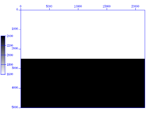
Figure 4: A two layers model.

The shot is set at the middle of the domain i.e. at $x_{s}=(10800,0)$ and the receivers are located at the depth $z=3000m$. By this way, we only account for the transmission effects. The transverse dimension of the model has been chosen such that the cardinal of the discrete set of points $x_{j}$ is matched for using FFTs. Each layer corresponds to a constant value of the velocity and their interface is located at $z=2500$m. The mesh dimensions are collected in the following table:

width of the computational domain	21.59 km
transverse step $\Delta x$	10 m
depth step $\Delta z$	10 m

In the following we refer to Velocity Model 1 (VM 1) when the velocity is equal to 1600 ms^-1 in the first layer and 2400 ms^-1 in the second one. VM 2 corresponds to the case where the velocity is equal to 1600 ms^-1 in the first layer and 5000 ms^-1 in the second one. The last model VM 3 is defined by a velocity equal to 2400 ms^-1 in the first layer and 1600 ms^-1 in the second one. VMs 1 and 3 are examples of velocities with a quite low contrast while VM 2 gives an example of high velocity contrast.

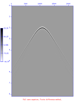
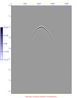
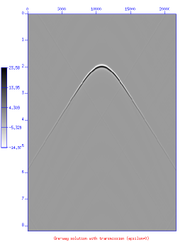
Figure 5: Seismograms.

On Fig.5, we have collected four seismograms. The first one depicts the reference solution obtained from the second-order full wave equation. On the right of this picture, we have set the solution of the one-way equations system as it was computed initially in [15]. One can observe that the kinematics is well-reproduced. Nevertheless the extrema of the grey scale shows that the amplitude of the one-way solution is erroneous. This motivates the two following pictures underneath. The left seismogram depicts the best results: both the kinematics and the amplitude of the wave field are correct. The right seismogram is not so bad even if the amplitude is more erroneous than in the previous case. Hence this first collection of numerical tests shows that to include the transmission term into the model really improves the amplitude of the wave field. Moreover if we limit our analysis to consider seismograms, we can conclude that the transmission term can be numerically handled as a term of the right-hand-side of the one-way system or as a proper term of the one-way equations. But the seismograms give a global view of the results and they are not precise enough to estimate the accuracy of the amplitude. This is why we have performed a series of numerical tests and we have chosen to represent them from the value of $Q$ which is defined by:

$$Q=\frac{\max\nolimits_{t}\left|p(t,x,0)\right|_{fullwave}}{\max\nolimits_{t}\left|p(t,x,0)\right|_{one-way}}.$$

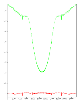
Figure 6: Values of $Q(x)$ in VM 1. Top curve: one-way solution without transmission. Lower curve: one-way solution with transmission (rhs).

On Fig. 6, the lower curve depicts the value of $Q$ for the one-way solution with $\epsilon=0$. Its values are very close to $1$ which confirms what was observed on the corresponding seismogram. The top curve represents the values of $Q$ for the one-way solution without the transmission term. This picture strengthens the previous conclusion since the minimum value of the error is $20\%$. Hence it is essential to include the transmission into the model to get accurate amplitudes.
Now, being convinced that the transmission must be included, the theory shows that it can be equivalently introduced whether into the one-way equations or into the rhs of the system. The first way allows to write a system of one-way equations which are quite close to the equations considered by Zhang and al. [18] as an approximation of the full wave equation. The second one is the most natural in the formalism of Bremmer series and was introduced by Le Rousseau and De Hoop [15, 8].

\begin{pspicture}(426.79115pt,227.62195pt) \rput[bl](0.0pt,0.0pt){\leavevmode} \end{pspicture}

Figure 7: Values of $Q(x)$ for the one-way solution with transmission in VM 1. Top curve: $\epsilon=0$. Lower curve: $\epsilon=1$

On Fig. 7, we have collected the values of $Q$ for $\epsilon=0$ and $\epsilon=1$. When $\epsilon=1$, the results are correct in a neighbourhood of the shot and then they spoil quickly. Hence this numerical test indicates that for VM 1, the best approach consists in including the transmission into the rhs.
Thus the result for $\epsilon=1$ may deteriorate more and more as fast as the velocity contrast is high. That motivates the next test on Fig. 8 where we can observe that actually the results spoil more and more: the minimum value of the error is now $8\%$ versus $1\%$ for VM 1.

\begin{pspicture}(426.79115pt,227.62195pt) \rput[bl](0.0pt,0.0pt){\leavevmode} \end{pspicture}

Figure 8: Values of $Q(x)$ for the one-way solution with transmission in VM 2. Top curve: $\epsilon=0$. Lower curve: $\epsilon=1$

On Fig. 9, we have collected three curves obtained from the one-way solution with $\epsilon=1$. Each of them are distinguished from the value of the velocity contrast. The pattern shows that the lower the contrast is the larger the neigbourhood of the shot in which the results are satisfactory is. This figure seems to indicate that the model with $\epsilon=1$ is correct when the propagation medium is smooth.

Figure 9: Values of $Q(x)$ for the one-way solution with $\epsilon=1$ and with different velocity contrasts

\begin{pspicture}(426.79115pt,284.52744pt) \rput[bl](0.0pt,0.0pt){\leavevmode} \end{pspicture}

Figure 10: Values of $Q(x)$ for the one-way solution with transmission in VM 3. Top curve: $\epsilon=0$. Lower curve: $\epsilon=1$

On Fig. 10 we have depicted the results for VM 3. It is just to show that the same conclusion holds even if the upper velocity is larger than the lower one. Let us mention that each curve shows some instabilities (depicted as local maxima) which are due to the periodicities created by the FFTs.

9 conclusion

In this paper we consider the numerical analysis of two one-way systems derived from the general modeling of M. De Hoop [8].
Such a formulation is used to replace the full wave equation by a system of one-way wave equations whose computational burden is lower than the one associated to the finite difference solution of the wave equation. Moreover it permits to unpack and identify the multiples from the primary reflections. We have include a transmission term in the one-way model. Then numerical tests have been performed in the 2D case and they indicate that accounting for the transmission improves significantly the amplitude of the solution. The computational algorithm has been optimized in such a way that its complexity is now of the same order than the one of the one-way solver without transmission. Hence to add the correcting term does not penalize the computational method. Now the solution is based on a method of propagators whose numerical approximation accuracy is very sensitive to the position of this correcting term. To put it into the one-way system, which is the case $\varepsilon=1$, seems to deteriorate the results. But this approach should be interesting since it corresponds to the same idea than the one proposed by Zhang et al. in [18] where time-arrivals are computed from the solution of a second-order wave equation obtained by factoring the full wave equation.

In this paper, we have performed a numerical test which shows that the accuracy of the method with $\epsilon=1$ is similar to the one of the method with $\epsilon=0$ when the velocity contrasts decrease.
In the proposed methods, the transmission operator is approximated by a zero order pseudodifferential operator which is exact for stratified media. A higher order operator, that should account for media with lateral velocity variations, is the topic of a current research [3].

References

- [1] K. Aki and P.G. Richards. Quantitative Seismology. University Science Books, 2002. Second edition.
- [2] X. Antoine and H. Barucq . Microlocal diagonalization of strictly hyperbolic pseudodifferential systems and application to the design of radiation conditions in electromagnetism. Siam J. on Appl. Math., 61(6):1877–1905, 2001.
- [3] H. Barucq , B. Duquet , and F. Prat . Comparison of the first order formulation of the wave equation with the complete first-order factorization of the full wave equation. in preparation.
- [4] H. Barucq , B. Duquet , and F. Prat . Coupling of one-way models with paraxial operators and absorbing boundary conditions. in preparation.
- [5] H. Barucq and O. Lafitte . High-order one-way systems taking the topography into account. in preparation.
- [6] H. Bremmer. The W.K.B. Approximation as the First Term of a Geometrical-Optical Series. Comm. Pure Appl. Math., 4:105–115, 1951.
- [7] J.P. Corones . Bremmer Series that correct Parabolic Approximations. J. Math. Annal. Appl., 50:361–372, 1975.
- [8] M.V. De Hoop. Generalizing of the Bremmer coupling series. J. Math.Phys., 37:3246–3282, 1996.
- [9] M.V. De Hoop, J.H. Le Rousseau, and R.S. Wu. Generalization of the phase-screen approximation for the scattering of acoustic waves. Wave Motion, 31:43–70, 2000.
- [10] V. Farra . Ray Tracing in Complex Media. J. of Applied Geophysics, 30:55–73, 1999.
- [11] R. Germain. Cours de Mécanique des milieux continus. Masson, Paris, 1973.
- [12] L. Hörmander. The analysis of linear partial differential operators, volume 3.& 4. Springer-Verlag, Berlin, 1985.
- [13] D. Kiyaschenko , R.E. Plessix , and B. Kastan. In EAGE 66th Conference and exihibition, Paris, 7-10 juin 2004.
- [14] O. Lafitte. Diffraction in the high frequency regime by a thin layer of dielectric material. I : the equivalent impedance boundary condition. Siam, J. Appl. Math., 59(3):1028–1052, 1999.
- [15] J.H. Le Rousseau. Microlocal analysis of wave-equation imaging and generalized-screen propagators. PhD thesis, Center for Wave phenomena, Colorado School of Mines, 2001.
- [16] F. Prat. Analyse du Generalized Screen Propagator. PhD thesis, Université de Pau et des Pays de l’Adour, 2005.
- [17] M.E. Taylor. Pseudo-differential operators. Princeton University Press, Princeton, NJ, 1981.
- [18] Y. Zhang , G. Zhang , and N. Bleistein . True amplitude wave equation migration arising from true amplitude one-way wave equations. Inverse Problems, 19:1113–1138, 2003.