Charge transport through weakly open one dimensional quantum wires

Abstract

We consider resonant transmission through a finite-length quantum wire connected to leads via finite transparency junctions. The coherent electron transport is strongly modified by the Coulomb interaction. The low-temperature current-voltage ($IV$) curves show step-like dependence on the bias voltage determined by the distance between the quantum levels inside the conductor, the pattern being dependent on the ratio between the charging energy and level spacing. If the system is tuned close to the resonance condition by the gate voltage, the low-voltage $IV$ curve is Ohmic. At large Coulomb energy and low temperatures, the conductance is temperature-independent for any relationship between temperature, level spacing, and coupling between the wire and the leads.

Quantization of conductance in ballistic one dimensional (1D) channels or islands disc is one of the central issues of current mesoscopic physics, see reviews for a review. In small-size islands, the Coulomb blockade suppresses conductivity at low temperatures and small applied voltages reviews2 . The Coulomb blockade can be controlled by varying the charge of the island between two tunnel barriers by the potential at the gate electrode; the conductance of such system shows oscillations as a function of the gate voltage, due to the periodic modulation of the charging energy. The classical theory of the Coulomb-blockade oscillations was developed in Shekhter , while the role of the discreteness of the spectrum was addressed in GS ; Beenakker91 and several subsequent papers. In these models the island was assumed to be almost isolated from both source and drain, so that the number of particles on it could be considered a conserved quantity. This assumption, in general, does not hold if the transparency of the contacts between the island and the leads is finite Matveev91 . Typical examples of such systems are quantum dots AGB .

Transport through quantum conductors (QCs) essentially coupled to the leads has not been fully investigated so far, though it offers excellent opportunities for studying the interplay between quantum and classical properties of QC. In this Letter, we investigate transport through a relatively short single-mode QC assuming a simplest model where charging effects are important whereas the Luttinger-liquid behavior is still not pronounced (see, e.g., LL ). We consider a ballistic conductor connected to two leads via identical contacts with a finite transition amplitude $\mathcal{T}$. Its length $d$ is shorter that the electron mean free path, the transport mechanism being the resonant transmission, which we distinguish from elastic cotunneling AverinNazarov90 . This mechanism is relevant to recent experiments on carbon nanotubes nanotubes1 ; nanotube .

At $\mathcal{T}\to 0$, the QC holds a fixed number of particles, $N$. If a particle with energy $E$ tunnels between a lead and the state with energy $\epsilon_{p}$ in the QC, the charging energy of the QC couples $E$ and $\epsilon_{p}$ through Beenakker91

$$E=\epsilon_{p}+2E_{C}(N-N_{0})\pm E_{C}$$ (1)

where $\pm$ stands for adding/removing a particle, $E_{C}=e^{2}/2C$ is the Coulomb energy of the QC, $C$ is the QC capacitance, and $eN_{0}$ is the gate-induced charge density. At finite $\cal T$, the system forms a double-barrier resonant tunneling structure, its properties being determined by the resonant states. The distance between these resonant levels is $\Delta E=\pi\hbar v/d$ (where $v$ is the electron velocity) while their width is $\Gamma=|{\cal T}|^{2}\Delta E$. The occupation probability of the modes is determined by the competition between the relaxation processes in the QC and in the leads, as well as by escape probability from the QC into the leads. If the inverse escape time, $\Gamma/\hbar$, is much less than the inter-mode relaxation time, $\tau^{-1}$, the occupation probability is the equilibrium Fermi distribution with the lattice temperature, the chemical potential being determined by the (conserved) number of particles. In the opposite case where $\Gamma\gg\hbar/\tau$ the distribution inside the QC is determined by the coupling to the leads; it can be strongly nonequilibrium. The distribution function is to be found from the kinetic equation. The results, in general, depend on interplay between the different relaxation mechanisms in the quantum conductor and the leads.

We will assume that the resonance width $\Gamma$ is small, but is still larger than the relaxation rate in the QC,

$$\hbar/\tau\ll\Gamma\ll\Delta E\,.$$ (2)

The requirement (2) is opposite to the condition $\Gamma\ll\hbar/\tau$ considered in Beenakker91 . In this limit QC cannot be treated as an isolated quantum dot with the vanishingly weak coupling to leads end1 , and therefore, $N$ is not a good quantum number but rather an average value determined by the interaction with the leads. To reflect this we employ the Hartree-Fock type approach which leads to modification of Eq. (1). We show that at finite $\mathcal{T}$ the excitation spectrum changes significantly. At large Coulomb energy, $E_{C}>\Delta E$, and low temperatures, $T\ll E_{C}$, energy exhibits a sharp step as a function of the internal momentum in the QC. This step defines the internal Fermi level. The width of the step is determined by the width of the resonant level. As a result, zero-voltage conductance becomes temperature-independent already at $T\ll E_{C}$ irrespective of the relationship between $T$, $\Delta E$, and $\Gamma$. In a carbon nanotube placed between the two leads the ratio $E_{C}/\Delta E=e^{2}d/2\pi\hbar v_{F}C$ can reach values $e^{2}/2\pi\hbar v_{F}$ for the minimal capacitance of the tube $C\sim d$. For typical $v_{F}=0.8\cdot 10^{8}$ cm/s nanotube this ratio is $\approx 0.46$, i.e., is of the order of unity. Therefore, in order to achieve better understanding of the experimental situation and having in mind more general applications, both limits of large and small ratio $E_{C}/\Delta E$ have to be studied.

Model.–

We specify the charging Hamiltonian as

$$\hat{H}_{C}=E_{C}\left[\sum_{\alpha}\int_{\mathcal{V}}\hat{\psi}^{\dagger}_{\alpha}({\bf r})\hat{\psi}_{\alpha}({\bf r})\,d\mathcal{V}-N_{0}\right]^{2}$$ (3)

$\mathcal{V}$ is volume of the QC and $\alpha$ is the spin index. The spin dependence is due to the level filling that controls the charge on the QC. The spectral and transport properties are determined by the retarded (advanced) and Keldysh Green functions satisfying the equations

$$\left\{\begin{array}[]{ll}\delta({\bf r}_{1}-{\bf r}_{2})\\ 0\end{array}\right\}=G_{0}^{-1}(\epsilon,{\bf r}_{1})\left\{\begin{array}[]{ll}G_{\epsilon}^{R(A)}({\bf r}_{1},{\bf r}_{2})\\ G_{\epsilon}^{K}({\bf r}_{1},{\bf r}_{2})\end{array}\right\}$$

$$\quad\quad+2E_{C}\int d\mathcal{V}\int\frac{d\epsilon_{1}}{4\pi i}G^{K}_{\epsilon_{1}}({\bf r}_{1},{\bf r})\left\{\begin{array}[]{ll}G_{\epsilon}^{R(A)}({\bf r},{\bf r}_{2})\\ G_{\epsilon}^{K}({\bf r},{\bf r}_{2})\end{array}\right\}\,,$$

$$G_{0}^{-1}(\epsilon,{\bf r}_{1})\equiv-\epsilon+\hbar^{2}\hat{\mathbf{p}}_{1}^{2}/2m-\mu+U_{C},\ \hat{\mathbf{p}}_{1}\equiv-i\partial/\partial\mathbf{r}_{1}.$$

The energy $U_{C}=e^{2}(N-N_{0})/C$ is produced by the charge on the QC, $\mu$ is the chemical potential; ${\bf r}_{1}$ belongs to the QC, otherwise the charging energy vanishes.

For methodical purposes, let us start with the example of infinitely long QC assuming $\Delta E\ll E_{C}$. Since $E_{C}$ is coordinate independent one can consider the wave functions as plane waves and use momentum representation. Then the Green function has the pole at $\epsilon=\varepsilon_{p}$ where

$$\varepsilon_{p}=\xi_{p}+U_{C}+E_{C}\tanh\frac{\varepsilon_{p}}{2T}\ ,\;\xi_{p}=\frac{\hbar^{2}p^{2}}{2m}-E_{F}\ .$$ (6)

$\varepsilon_{p}$ is measured from the Fermi level $\mu=E_{F}$ in the leads. At $\varepsilon_{p}\gg T$ this coincides with Eq. (1). For $\varepsilon_{p}\rightarrow 0$ one has $\varepsilon_{p}=(\xi_{p}+U_{C})/(1-E_{C}/2T)$. The slope of the $\varepsilon_{p}$ vs $\xi_{p}$ dependence is negative for $E_{C}>2T$, and the function $\varepsilon_{p}$ becomes multi-valued, see Fig. 1(a). As we will see later, $\varepsilon_{p}$ in fact experiences an abrupt jump as a function of internal momentum shown in Fig. 1(a) by the vertical line. This infinite slope is a consequence of the chosen approximation of an infinitely long QC with $\Delta E\to 0$.

In a finite QC, the jump acquires a finite width determined by the transparency of the contacts. To study this problem in more detail it is convenient to expand Green’s functions over the orthonormal set of functions $u_{n}(\mathbf{r})$, which satisfy the Schrödinger equation

$$\left(\frac{\hbar^{2}\hat{\mathbf{p}}^{2}}{2m}-\mu+U_{C}\right)u_{n}+E_{C}\sum_{m}u_{m}N_{mn}=E_{n}u_{n}\,.$$ (7)

Here $N_{mn}=\int d\mathcal{V}\,u^{*}_{m}({\bf r})u_{n}({\bf r})f(E_{m})$; $f(E_{m})\equiv 1-2n(E_{m})$, where $n(E_{m})$ is the occupation probability of the $m$-th state. The diagonal element is proportional to the average charge $eN_{nn}$ in the state $n$.

Spectrum.

– Since main contributions to the transport come from the quasi-resonant tunneling states it is convenient to expand the functions $u_{n}$ over the scattering plane-wave states, $v_{p}(x)$, satisfying the equation

$$\left[\frac{\hbar^{2}\hat{\mathbf{p}}^{2}}{2m}-\mu+V\sum_{\pm}\delta(x\pm d/2)\right]v_{p}(x)=\xi_{p}v_{p}(x)\,.$$ (8)

The wave functions can be chosen as incident waves on the left, $v_{p}$, and incident waves on the right, $v_{\bar{p}}$. We assume a symmetric structure such that each barrier is characterized by the same plane-wave reflection $\mathcal{R}$ and transmission ${\cal T}$ amplitudes, $\mathcal{R}=|\mathcal{R}|e^{i\delta}$ and ${\cal T}=-|{\cal T}|e^{i\delta}$ where $\delta$ is the scattering phase; $|\mathcal{R}|^{2}+|{\cal T}|^{2}=1$. We now express the wave functions $u_{n}$ through the free functions $v_{p}$: $u_{n}(x)=(2\pi)^{-1}\int A_{np}v_{p}(x)\,dp$. Using the orthogonality and completeness of both sets $u_{n}$ and $v_{p}$ one can show that the states $u_{n}$ with the different $n$ are expanded in $v_{p}$ with different $p$. This property, in particular, excludes the multi-valued solutions of Eq. (6) shown in Fig. 1(a). Equation (7) can be then rewritten in the form

$$\epsilon_{p}-E_{n}=\int\frac{dp^{\prime}}{2\pi}\frac{A_{np^{\prime}}}{A_{np}}\left[(e\varphi-U_{C})M_{pp^{\prime}}-E_{C}Q_{pp^{\prime}}\right];$$

$$M_{pp^{\prime}}\equiv\int_{-d/2}^{d/2}v_{p}^{*}(x)v_{p^{\prime}}(x)\,dx\,,$$ (9)

$$Q_{pp^{\prime}}\equiv\sum_{m}\int\frac{dp_{1}}{2\pi}\frac{dp_{2}}{2\pi}A_{mp_{1}}A^{*}_{mp_{2}}f_{1}(E_{m})M_{pp_{1}}M_{p_{2}p^{\prime}}.$$

The matrix elements $M_{pp^{\prime}}$ can be explicitly expressed through the transition amplitude, $\mathcal{T}$.

In the equilibrium, the distribution functions for particles coming from the left and right are the same, $f(E)=\tanh(E/2T)$. In what follows we concentrate on the situation when the transparency satisfies Eq. (2). For $|\mathcal{T}|\ll 1$ there exist sharp resonances in the transmission when the momentum of electrons inside the QC is close to the resonant values corresponding to integer ratio $s\equiv(pd+\delta)/\pi$, $\delta\approx\pi$. We denote $p_{n}^{\pm}$ the even and odd resonant states for $s=2n+1$ and $s=2n$, respectively. At $E_{C}\gg\Delta E$ these internal resonance momenta of $u_{n}(r)$ lie far from the incident particle momenta in the leads $\sqrt{2m(E+E_{F})}$ but are close to the resonance momenta of the plane-wave states, $v_{p}(x)$. This implies that transport is controlled only by discrete resonant levels, which distinguishes the considered mechanism from the usual elastic cotunneling through a multi-level quantum dot AverinNazarov90 . Consequently, one can put $A_{np}\approx M_{q_{n}p}^{*}=M_{pq_{n}}$ where the continuous parameter $q_{n}$ is the wave vector of a particle inside the QC close to $n$-th resonance. Equation (Spectrum.) for $p=q_{n}$ becomes (for both even and odd states)

$$E_{n}=\epsilon_{q_{n}}+U_{C}-e\varphi+E_{C}\int\frac{dp}{2\pi}f(E_{p})M_{pp}^{\pm}\,;$$ (10)

$$M_{pp^{\prime}}^{\pm}=\frac{{\cal T}_{p^{\prime}}{\cal T}^{*}_{p}e^{i(p-p^{\prime})d/2}\Delta(p-p^{\prime})}{(e^{-ip^{\prime}d/2}\mp\mathcal{R}e^{ip^{\prime}d/2})(e^{ipd/2}\mp\mathcal{R}^{*}e^{-ipd/2})}\,.$$

Here $\epsilon_{q_{n}}=\hbar^{2}q_{n}^{2}/2m-E_{F}$, the integration is performed over the vicinity of the $n$-th resonance, $p_{n}^{\pm}$; $\Delta(p)\equiv(2/p)\sin(pd/2)$. Equation (10) generalizes Eq. (6) with the replacements $\varepsilon_{p}\to E_{m}$, $\xi_{p}\to\epsilon_{q_{n}}$ and defines $q_{n}$ corresponding to the resonant transmission through the QC.

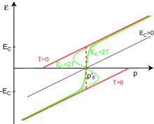
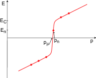
Figure 1: (Color online) (a) Energy spectrum of an infinitely long normal conductor. Finite temperature: The slope at $E=0$ is positive for $E_{C}<2T$ (green line) and negative for $2T<E_{C}$ (dotted line). For $T=0$ (red lines) the Fermi surface corresponds to the jump in the spectrum; $p_{\mu}^{\prime}=p_{\mu}-U_{C}/v$ (dashed vertical line). Straight (black) line: zero Coulomb energy. (b) Energy spectrum for a finite-transparency contacts. The dots illustrate sequential position of even and odd states.

If the intra-QC relaxation is efficient, $\tau_{\epsilon}\ll\hbar/\Gamma$, where $\tau_{\epsilon}$ is the inelastic relaxation time in the QC, the distribution is determined by the states in the QC, $f(E_{p})\equiv f(\epsilon_{q_{n}})=\tanh(\epsilon_{q_{n}}/2T)$. The abrupt dependence shown in Fig. 1(a) is then smeared by the finite temperature, and $E_{n}$ as a function of $q_{n}$ acquires a finite width $\sim T$, similarly to the situation considered in Beenakker91 . However, if Eq. (2) holds, and when temperature satisfies $T\ll E_{C}$, the spectrum $E_{n}(q_{n})$ shows a jump over $2E_{c}$ at some value $q_{n}\equiv p_{\mu}$ such that all the levels with $q_{n}>p_{\mu}$ are empty, while the levels with $q_{n}<p_{\mu}$ are occupied. Therefore $f(E_{n})\approx\mathrm{sign}(q_{n}-p_{\mu})$. With this approximation in the r.h.s. of Eq. (10) one finds for $\mathcal{T}\ll 1$

$$E_{n}=\hbar v(q_{n}-p_{F})-e\varphi+U_{C}+E_{C}\Phi(p_{n}-p_{\mu})\,.$$ (11)

Here $q_{n}$ is close to the resonance value $p_{n}\equiv\pi n/d$ and

$$\Phi(p_{n}-p_{\mu})=(2/\pi)\arctan\left[2d(p_{n}-p_{\mu})/|\mathcal{T}|^{2}\right]\ .$$ (12)

Equation (11) generalizes Eq. (1) for low transparency limited by Eq. (2); Eqs. (11) and (1) coincide far from the Fermi level. Energies $E_{n}$ for the resonance momenta $p_{n}$ are shown in Fig. 1(b). The width of this function is determined by $\Gamma$, rather than by the temperature.

The Fermi momentum, $p_{\mu}$, is related to the number of electrons inside the QC. We define the variation of the particle number, $\delta N$, as a function of the bias and gate voltage. Using Eqs. (11), (12) one can cast this variation in the form $\delta N=-(1/2)\delta\left[\sum_{n,\alpha}\Phi(p_{n}-p_{\mu})\right]$. Here the sum runs also over the electron spin index $\alpha$. Let us denote the average number of electrons for zero gate voltage as $N_{0}$. If $N_{0}$ is an integer, the chemical potential lies far from one of the resonances $|\mathcal{T}|^{2}/d\ll|p_{\mu}-p_{n}|\leq\pi n/2d$. For non-integer $N_{0}$, one can split it into the integer part, $[N_{0}]$, and the remainder, $\tilde{N}_{0}$. In this case, the chemical potential is close to one of the resonances. Assuming that the state $n$ is the closest to the Fermi level one can determine $p_{\mu}$ from the equation $\Phi(p_{n}-p_{\mu})=1-2\tilde{N}_{0}$. In general, the chemical potential and the number of particles are related by the equation $2(N-[N_{0}])+\Phi(p_{n}-p_{\mu})=1$. Near the degeneracy point when $N-[N_{0}]=\pm 1/2$, the Fermi momentum is close to one of the resonances.

Current.

For a finite bias $V$, energies in the left and right leads are shifted by $\pm eV/2$. Following the same approximation as above, we have instead of Eq. (11)

$$E_{n}=\hbar v_{F}(q_{n}-p_{F})-e\varphi+U_{C}+\frac{E_{C}}{2}\!\!\!\sum_{i=L(R)}\!\!\!\Phi\left(p_{n}-p_{\mu}^{(i)}\right).$$

Now the Fermi momenta, $p_{\mu}^{L}$ and $p_{\mu}^{R}$, are not equal but are determined by the states in the left and right electrode, respectively. Similarly to the equilibrium case, we get $\delta N=-(1/4)\delta\left[\sum_{n,\alpha,i=L(R)}\Phi\left(p_{n}-p_{\mu}^{(i)}\right)\right]$. Defining $j_{p}\equiv u_{p}^{*}(x)[\partial u_{p}(x)/\partial x]$ one can express current as

$$I=-\frac{e\hbar}{m}\sum_{p,\alpha}\left[f_{1}^{L}(E_{p})\mathop{\mathrm{Im}}j_{p}+f_{1}^{R}(E_{\bar{p}})\mathop{\mathrm{Im}}j_{\bar{p}}\right],$$ (13)

The following analysis is different for small and large values of $E_{C}/(\Delta E)$. At $E_{C}\ll\Delta E$, the energy $E_{n}=\hbar v(q_{n}-p_{\mu})$ is independent of the level population and thus of the spin state. At relatively high temperatures, $\Gamma\ll T\ll\Delta E$, using Eq. (13), one obtains

$$I=\frac{I_{0}}{2}\sum_{n}\left[\tanh\frac{E_{n}^{+}}{2T}-\tanh\frac{E_{n}^{-}}{2T}\right],\ I_{0}\equiv\frac{ev}{2d}|{\cal T}|^{2}.$$ (14)

$E_{n}^{\pm}\equiv E_{n}\pm eV/2$, $n$ runs over even and odd states. The $IV$-curves are shown in Fig. 2. The current exhibits steps at $eV=2(\Delta En\pm\delta E)$ where $\delta E=(\hbar v/\pi)[p_{\mu}-\pi M/d]$ is the deviation from resonance between the zero-voltage Fermi energy in the leads and one of the levels, $M$ being an integer.

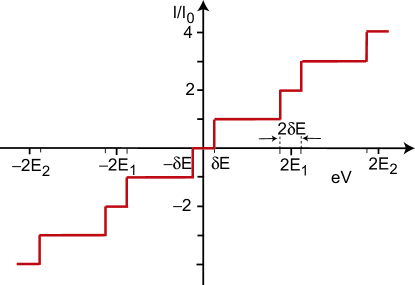
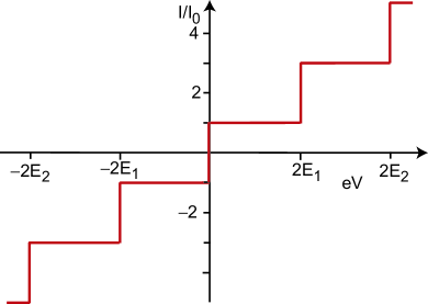
Figure 2: (Color online) (a) Current steps for zero Coulomb energy and $T=0$. $E_{n}=\Delta En$ is the resonance energy, $\delta E=\hbar v\alpha^{\prime}/d$ is the deviation from the resonance. (b) For exact resonance, $\delta E=0$, the steps are doubled.

For $T\ll\delta E$ and small voltages, $eV\leq\delta E$, the current is zero. For the resonance, $\delta E=0$, the current is given by the term with $n=M$ in the sum, $I=I_{0}\tanh\left(eV/4T\right)$. At $eV\ll T$ the conductance is Ohmic, $G=eI_{0}/4T$, which agrees with Refs. Beenakker91 ; CN2barrier .

For large $E_{C}$, the states within the interval $\delta p\sim|\mathcal{T}|^{2}/d$ near the lowest resonance level, i.e., those which contribute to the current, have energies $\sim E_{C}$. Therefore the distribution function $\mathop{\mathrm{sign}}(q_{n}-p_{\mu})$ can be used up to temperatures $T\ll E_{C}$, regardless of the relation between $T$ and $\Gamma$ or $\Delta E$. Using Eq. (13) we find

$$I=(I_{0}/4)\sum_{n,\alpha}\left[\Phi(p_{n}-p_{\mu}^{R})-\Phi(p_{n}-p_{\mu}^{L})\right]\,.$$ (15)

The level positions are determined by the condition of minimal total energy which fixes the value of $N-N_{0}$. Thus the levels, as functions of the bias voltage, will cross the Fermi energy pairwise, one level from above while the other from below, keeping the number of electrons $N-N_{0}$ unchanged and lifting the Coulomb blockade in the bias voltage. If the Fermi level lies between the resonances, the first step of hight $I_{0}$ in the current appears for $V=\Delta E/e$. The next steps appear when the bias voltage is increased by $\delta V=2\Delta En/e$. The heights of the current steps are the same as for low $E_{C}$: the extra factor $\frac{1}{2}$ in Eq.(15) is compensated by the pairwise level crossing. However, the fine structure shown in Fig. 2(a) disappears.

If the system is close to the degeneracy point $N-[N_{0}]=\pm 1/2$, when one of the values $p_{n}$ is close to $p_{\mu}$, even a small bias voltage is sufficient to produce current. We find from Eq. (15) for low voltage, $eV\ll\Gamma$,

$$I=\frac{G_{0}V}{2}\frac{|{\cal T}|^{4}}{|{\cal T}|^{4}+4(p_{n}-p_{\mu})^{2}d^{2}}\,,\quad G_{0}\equiv\frac{e^{2}}{\pi\hbar}\,.$$ (16)

In the resonance, $p_{n}=p_{\mu}$, the conductance is half of the conductance quantum, $G_{0}/2$. The conductance does not depend on temperature at $T\leq E_{C}$. This fact differs from the tunnel-approximation result of Ref. Beenakker91 for the temperature domain $\Gamma\ll T\ll E_{C}$. The difference is due to the step in the energy spectrum caused by relatively strong coupling to the leads. Probing the onset of Ohmic conductance at the degeneracy point allows one to monitor the effective number of electrons in the QC.

Conclusion.

We develop a mean field type description of the Coulomb effects in the “weakly open” 1D systems and analyze both the excitation energy spectrum and the electric current. The $IV$ curves show a step-like dependence on the bias voltage, the exact shape being determined by the ratio between the charging energy and the level spacing. At large charging energy and low temperatures $T\ll E_{C}$, the low-voltage Ohmic conductance, Eq. (16), is temperature-independent irrespectively to the magnitude of the ratios $T/\Delta E$ and $T/\Gamma$.

- (1) B. J. van Wees et al., Phys. Rev. Lett. 60, 848 (1988); D. A. Wharam et al., J. Phys. C 21, L209 (1988).
- (2) H. van Houten et al., in Semiconductors and Semimetals, ed. by M. A. Reed (Academic, New York); C. W. J. Beenakker and H. van Houten, in Solid State Physics, ed. by D. Turnbull and H. Ehrenreich (Academic, New York).
- (3) K. K. Likharev, IBM J. Res. Dev. 32, 144 (1988); D. V. Averin and K. K. Likharev, in Mesoscopic Phenomena in Solids, ed. by B. L. Altshuler et al. (Elsevier, Amsterdam, 1991); H. van Houten et al., in Single Charge Tunneling, NATO Advanced Study Institute, Series B: Physics, ed. by H. Grabert and M. H. Devoret (Plenum, New York, 1991).
- (4) R. I. Shekhter, Zh. Eksp. Teor. Fiz. 63, 1410 (1972) [Sov. Phys.-JETP 36, 747 (1973)]; I. O. Kulik and R. I. Shekhter, Zh. Eksp. Teor. Fiz. 68, 623 (1975) [Sov. Phys.-JETP 41, 308 (1975)].
- (5) L. I. Glazman and R. I. Shekhter, J. Phys. Conden. Matter 1, 5811 (1989).
- (6) C. W. J. Beenakker, Phys. Rev. B 44, 1646 (1991).
- (7) K. A. Matveev, Zh. Eksp. Teor. Fiz. 99, 1598 (1991) [Sov. Phys. JETP, 72, 892 (1991)]; Phys. Rev. B 51, 1743 (1995).
- (8) I. L. Aleiner et al., Physics Reports, 358/5-6 309, (2002).
- (9) M. Ogata and H. Fukuyama, Phys. Rev. Lett. 73, 468 (1994); V. V. Ponomarenko and N. Nagaosa, Phys. Rev. B56, R12756 (1997).
- (10) D. V. Averin and Yu. V. Nazarov, Phys. Rev. Lett. 65, 2446 (1990).
- (11) M. Bockrath et al., Nature (London) 397, 598 (1999); Z. Yao et al., Nature (London) 402, 273 (1999).
- (12) P. Jarillo-Herrero et al., Nature, 439, 953 (2006).
- (13) Consequently one cannot use the tunneling Hamiltonian formalism as in I. Weymann et al., Phys. Rev. B76, 155408 (2007); preprint arXiv:0803.1969v1; N. A. Zimbovskaya, preprint arXiv:0803.3799.
- (14) H. W. Ch. Postma et al., Science 293, 76 (2001).