Generalized Phase Rules

Abstract

For a multi-component system, general formulas are derived for the dimension of a coexisting region in the phase diagram in various state spaces.

1 Introduction

The first-order phase transition plays an important role in diverse fields of physics. Its most characteristic feature is that a phase boundary is a coexisting region, where two or more phases coexist. The dimension $D$ of a coexisting region in the phase diagram depends on the number $r$ of coexisting phases [1, 2, 3, 4, 5]. It also depends on which variables are taken as the axes of the phase diagram [1, 2, 3].

For example, for a single-component system whose natural variables of the entropy [1, 2, 3, 4] are $U$ (energy), $V$ (volume) and $N$ (amount of substance), the phase diagram may be drawn either in the $T$-$P$ plane, or in the $T$-$v$ plane, or in the $u$-$v$ plane, where $T,P,v$ and $u$ are the temperature, pressure, molar volume ($\equiv V/N$) and molar energy ($\equiv U/N$), respectively. Here, $v$ and/or $u$ are used instead of $V$ and/or $U$ in order to make the diagrams independent of $N$. These phase diagrams are schematically shown in Figs. 1, 2 and 3, respectively [3]. We denote $D$ for these diagrams by $D(T,P)$, $D(T,v)$ and $D(u,v)$, respectively. For example, $D(T,P)=1,D(T,v)=D(u,v)=2$ for a liquid-gas coexisting region, where two phases coexist (i.e., $r=2$), whereas $D(T,P)=0,D(T,v)=1,D(u,v)=2$ at the triple point, where $r=3$.[1, 2, 3] Since $T$ and $P$ can take constant values across a coexisting region,[1, 2, 3] $D$ of the coexisting region tends to shrink if $T$ and/or $P$ is taken as an axis(es) of the phase diagram, and thus $D(T,P)\leq D(T,v)\leq D(u,v)$.

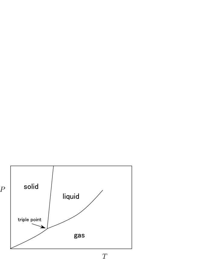
Figure 1: A schematic phase diagram of a single-component system, plotted in the space spanned by the axes corresponding to $T$ and $P$. The solid-liquid-gas coexisting region is a point, which is called the triple point. On the other hand, the liquid-gas, solid-liquid and solid-gas coexisting regions are lines, which are called coexisting lines.

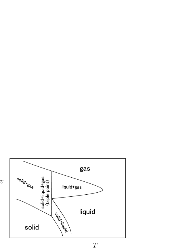
Figure 2: A schematic phase diagram of a single-component system, plotted in the space spanned by the axes corresponding to $T$ and $v$ $(\equiv V/N)$. Unlike Fig. 1, the solid-liquid-gas coexisting region (triple point) is a vertical line, whereas the liquid-gas, solid-liquid and solid-gas coexisting regions are planes.

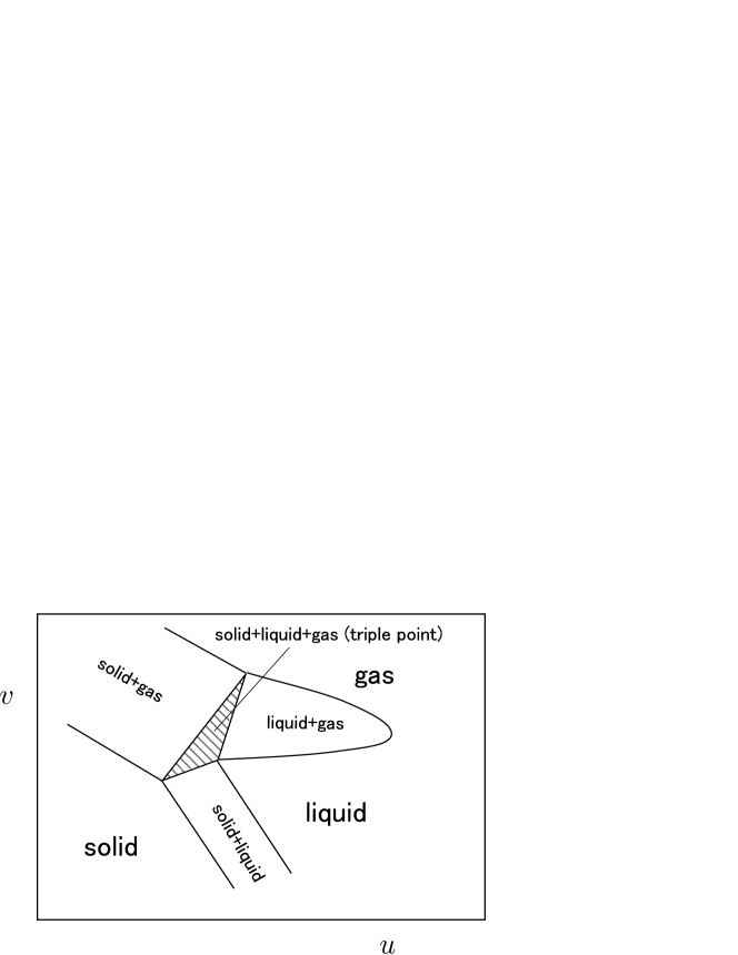
Figure 3: A schematic phase diagram of a single-component system, plotted in the space spanned by the axes corresponding to $u$ $(\equiv U/N)$ and $v$ $(\equiv V/N)$. All the coexisting regions are planes. For example, the triple point, which was a point in Fig. 1, extends to the shaded area in this figure. Unlike Figs. 1 and 2, every point in this diagram corresponds to a single equilibrium state, and different points correspond to different equilibrium states.

For such a single-component system, $D(T,P)$ coincides with the ‘thermodynamical degrees of freedom’ $f$, which is given by the Gibbs phase rule [1, 2, 3, 4, 5] (see eq. (7) below). On the other hand, $D(u,v)\geq D(T,v)\geq f$ in general [1, 3]. For example, $f=1=D(T,P)<D(T,v)=D(u,v)=2$ for a liquid-gas coexisting region, whereas $f=0=D(T,P)<D(T,v)<D(u,v)=2$ at the triple point.

The situation becomes more complicated for a multi-component system, which consists of $q$ ($\geq 2$) different substances. We assume that the natural variables of entropy are $U,V,N_{1},\ldots,N_{q}$, where $N_{j}$ ($j=1,\ldots,q$) is the amount of substance $j$. That is, the entropy $S$ is a function of these additive (extensive) variables;

$$S=S(U,V,N_{1},\ldots,N_{q}),$$ (1)

which is called the fundamental relation [1, 3, 4]. Let $N_{\rm tot}$ be the total amount of substances,

$$N_{\rm tot}\equiv N_{1}+\ldots+N_{q}.$$ (2)

To make phase diagrams independent of $N_{\rm tot}$, we use the normalized variables;

$$u \equiv {U\over N_{\rm tot}},$$ (3)

$$v \equiv {V\over N_{\rm tot}},$$ (4)

$$n_{j} \equiv {N_{j}\over N_{\rm tot}}\quad(j=1,\ldots,q).$$ (5)

Among $n_{1},\ldots,n_{q}$, only $(q-1)$ variables are independent because of the identity

$$\sum_{j=1}^{q}n_{j}=1.$$ (6)

Hence, the phase diagram may be drawn in the $(q+1)$-dimensional space that is spanned by the axes corresponding to either $(T,P,n_{1},\ldots,n_{q-1})$, $(T,v,n_{1},\ldots,n_{q-1})$, or $(u,v,n_{1},\ldots,n_{q-1})$, which correspond to the so-called $TPN$, $TVN$ and $UVN$ representations, respectively. We denote the dimensions of a coexisting region in these spaces by $D(T,P,n_{1},\ldots,n_{q-1})$, $D(T,v,n_{1},\ldots,n_{q-1})$ and $D(u,v,n_{1},\ldots,n_{q-1})$, respectively.

On the other hand, the thermodynamical degrees of freedom[1, 2, 3, 4, 5] $f$ is defined as the number of variables that can be varied independently in the coexisting region, among the intensive variables $T,P,\mu_{1},\ldots,\mu_{q}$, where $\mu_{j}$ denotes the chemical potential of substance $j$. The Gibbs phase rule gives [1, 2, 3, 4, 5]

$$f=q+2-r.$$ (7)

For $q\geq 2$ neither of $D$’s coincides with $f$ in general, and the explicit formulas for $D$’s were unknown.

Knowledge about $D$’s would be very helpful in drawing phase diagrams of new materials [1, 2, 3, 4, 5]. Since phase diagrams are most fundamental to studies of macroscopic systems, general formulas would be valuable which give $D(T,P,n_{1},\ldots,n_{q-1})$, $D(T,v,n_{1},\ldots,n_{q-1})$ and $D(u,v,n_{1},\ldots,n_{q-1})$ as functions of $q$ and $r$. The purpose of the present paper is to derive such general formulas. We also evaluate $D$’s in some other spaces. The results will be summarized as the chain of equalities and inequalities, eq. (41).

2 $UVN$ representation

2.1 Basic relations

We consider a $q$-component system, the natural variables of whose entropy [1, 2, 3, 4] are assumed to be $U,V,N_{1},\ldots,N_{q}$. For each coexisting region, we label the coexisting phases by $\alpha=1,\ldots,r$. For example, the shaded region of Fig. 3 is a coexisting region, in which the gas ($\alpha=1$), liquid ($\alpha=2$) and solid ($\alpha=3$) phases coexist, hence is called the triple point. Note that there is the trivial $r!$-fold degeneracy in labeling $\alpha=1,\ldots,r$. Since this degeneracy does not affect the values of $D$’s, we henceforth forget about it.

The values of $U,V$ and $N_{j}$ in phase $\alpha$ are denoted by $U^{\alpha},V^{\alpha}$ and $N^{\alpha}_{j}$, respectively. They are related to those of the total system as

$$U = \sum_{\alpha=1}^{r}U^{\alpha},$$ (8)

$$V = \sum_{\alpha=1}^{r}V^{\alpha},$$ (9)

$$N_{j} = \sum_{\alpha=1}^{r}N^{\alpha}_{j}\quad(j=1,\ldots,q).$$ (10)

Corresponding to $u,v,n_{j}$ of the total system, we define

$$u^{\alpha} \equiv {U^{\alpha}\over N^{\alpha}_{\rm tot}},$$ (11)

$$v^{\alpha} \equiv {V^{\alpha}\over N^{\alpha}_{\rm tot}},$$ (12)

$$n^{\alpha}_{j} \equiv {N^{\alpha}_{j}\over N^{\alpha}_{\rm tot}}\quad(j=1,\ldots,q)$$ (13)

for each phase, where $N^{\alpha}_{\rm tot}$ is the total amount of substances in phase $\alpha$,

$$N^{\alpha}_{\rm tot}\equiv N^{\alpha}_{1}+\ldots+N^{\alpha}_{q}\quad(\alpha=1,\ldots,r).$$ (14)

Corresponding to eq. (6), we have

$$\sum_{j=1}^{q}n^{\alpha}_{j}=1\ \mbox{ for all $\alpha$}.$$ (15)

We also define the molar fraction of each phase

$$\nu^{\alpha}\equiv{N^{\alpha}_{\rm tot}\over N_{\rm tot}}\quad(\alpha=1,\ldots,r)$$ (16)

which satisfies the trivial identity

$$\sum_{\alpha=1}^{r}\nu^{\alpha}=1.$$ (17)

By dividing eqs. (8)-(10) by $N_{\rm tot}$, we obtain

$$u = \sum_{\alpha=1}^{r}\nu^{\alpha}u^{\alpha},$$ (18)

$$v = \sum_{\alpha=1}^{r}\nu^{\alpha}v^{\alpha},$$ (19)

$$n_{j} = \sum_{\alpha=1}^{r}\nu^{\alpha}n_{j}^{\alpha}\quad(j=1,\ldots,q).$$ (20)

Note that each phase is, by definition [3, 5, 6], homogeneous spatially. Hence, the local value of the molar energy is equal to $u^{\alpha}$ at everywhere in phase $\alpha$. On the other hand, the total system is inhomogeneous in a coexisting region, and the local value of the molar energy is equal not to $u$ but to either of $u^{1},u^{2},\ldots$, or $u^{r}$. As seen from eq. (18), $u$ actually represents the average molar energy, which is the weighted average of $u^{\alpha}$’s of the coexisting phases. The same can also be said about $v$ and $n_{j}$.

Intensive variables in phase $\alpha$ are continuous functions of $u^{\alpha},v^{\alpha},n^{\alpha}_{1},\ldots,n^{\alpha}_{q-1}$ [1, 3], and have the same values as those of the total system [1, 2, 3, 4];

$$T=T(u^{\alpha},v^{\alpha},n^{\alpha}_{1},\ldots,n^{\alpha}_{q-1})=T(u,v,n_{1},\ldots,n_{q-1}),$$ (21)

$$P=P(u^{\alpha},v^{\alpha},n^{\alpha}_{1},\ldots,n^{\alpha}_{q-1})=P(u,v,n_{1},\ldots,n_{q-1}),$$ (22)

$$\mu_{j}=\mu_{j}(u^{\alpha},v^{\alpha},n^{\alpha}_{1},\ldots,n^{\alpha}_{q-1})=\mu_{j}(u,v,n_{1},\ldots,n_{q-1})\quad(j=1,\ldots,q).$$ (23)

Here, the functions $T(\cdot,\cdot,\ldots,\cdot)$, $P(\cdot,\cdot,\ldots,\cdot)$ and $\mu_{j}(\cdot,\cdot,\ldots,\cdot)$ are obtained by differentiating the fundamental relation, eq. (1) [1, 3, 4].

2.2 $D$ in the $\{u^{\alpha},v^{\alpha},n^{\alpha}_{1},\ldots,n^{\alpha}_{q-1},\nu^{\alpha}\}_{\alpha=1,\ldots,r}$ space

Our principal purpose is to evaluate $D$’s in the $(q+1)$-dimensional spaces such as the one spanned by the axes corresponding to $(T,P,n_{1},\ldots,n_{q-1})$. As a preliminary, we first evaluate the dimension $D(\{u^{\alpha},v^{\alpha},n^{\alpha}_{1},\ldots,n^{\alpha}_{q-1},\nu^{\alpha}\}_{\alpha})$ in a larger space which is spanned by the axes corresponding to $r(q+2)$ variables $\{u^{\alpha},v^{\alpha},n^{\alpha}_{1},\ldots,n^{\alpha}_{q-1},\nu^{\alpha}_{\rm tot}\}_{\alpha=1,\ldots,r}$ [7].

Since $r$ different phases coexist, we have

$$T(u^{1},v^{1},n^{1}_{1},\ldots,n^{1}_{q-1})=\ldots=T(u^{r},v^{r},n^{r}_{1},\ldots,n^{r}_{q-1}),$$ (24)

$$P(u^{1},v^{1},n^{1}_{1},\ldots,n^{1}_{q-1})=\ldots=P(u^{r},v^{r},n^{r}_{1},\ldots,n^{r}_{q-1}),$$ (25)

$$\mu_{j}(u^{1},v^{1},n^{1}_{1},\ldots,n^{1}_{q-1})=\ldots=\mu_{j}(u^{r},v^{r},n^{r}_{1},\ldots,n^{r}_{q-1})\quad(j=1,\ldots,q),$$ (26)

which impose $(r-1)\times(q+2)$ conditions on $r\times(q+1)$ variables $\{u^{\alpha},v^{\alpha},n^{\alpha}_{1},\ldots,n^{\alpha}_{q-1}\}_{\alpha=1,\ldots,r}$. Therefore, the dimension of the set of values of $\{u^{\alpha},v^{\alpha},n^{\alpha}_{1},\ldots,n^{\alpha}_{q-1}\}_{\alpha=1,\ldots,r}$ is evaluated as

$$r(q+1)-(r-1)(q+2)=q+2-r.$$ (27)

Among the residual variables $\nu^{1},\ldots,\nu^{r}$, we have eq. (17). Hence,

$$D(\{u^{\alpha},v^{\alpha},n^{\alpha}_{1},\ldots,n^{\alpha}_{q-1},\nu^{\alpha}\}_{\alpha}) = (q+2-r)+(r-1)$$ (28)

$$= q+1.$$

2.3 $D$ in the $u,v,n_{1},\ldots,n_{q-1}$ space

With the help of eq. (28), we can evaluate $D(u,v,n_{1},\ldots,n_{q-1})$ as follows. It is obvious from eqs. (8)-(10) that the values of $U,V,N_{1},\ldots,N_{q}$ are uniquely determined by the values of $\{U^{\alpha},V^{\alpha},N_{1}^{\alpha},\ldots,N_{q}^{\alpha}\}_{\alpha=1,\ldots,r}$. Furthermore, the latter (including the number $r$) is uniquely determined by the former, because otherwise two different states would have the same value of the total entropy $S(U,V,N_{1},\ldots,N_{q})$, and thus the total system would be unstable [3]. Therefore, the values of $\{U^{\alpha},V^{\alpha},N_{1}^{\alpha},\ldots,N_{q}^{\alpha}\}_{\alpha=1,\ldots,r}$ (including $r$) have one-to-one correspondence with the values of $U,V,N_{1},\ldots,N_{q}$ of the total system. This means that $\{u^{\alpha},v^{\alpha},n^{\alpha}_{1},\ldots,n^{\alpha}_{q-1},N^{\alpha}_{\rm tot}\}_{\alpha=1,\ldots,r}$ have one-to-one correspondence with $u,v,n_{1},\ldots,n_{q-1},N_{\rm tot}$. Hence, $\{u^{\alpha},v^{\alpha},n^{\alpha}_{1},\ldots,n^{\alpha}_{q-1},\nu^{\alpha}\}_{\alpha=1,\ldots,r}$ have one-to-one correspondence with $u,v,n_{1},\ldots,n_{q-1}$. Therefore,

$$D(u,v,n_{1},\ldots,n_{q-1}) = D(\{u^{\alpha},v^{\alpha},n^{\alpha}_{1},\ldots,n^{\alpha}_{q-1},\nu^{\alpha}\}_{\alpha})$$ (29)

$$= q+1,$$

which is equal to the dimension of all possible states for a given value of $N_{\rm tot}$ [1, 3, 4]. This is reasonable (obvious in some sense) because each equilibrium state has one-to-one correspondence with the set of values of $U,V,N_{1},\ldots,N_{q}$, even when the equilibrium state is in a coexisting region [1, 3].

For a single-component system, for example, formula (29) gives $D(u,v)=2,$ which is consistent with Fig. 3.

3 $TVN$ representation

3.1 $D$ in the $T,\{v^{\alpha},n^{\alpha}_{1},\ldots,n^{\alpha}_{q-1}\}_{\alpha=1,\ldots,r}$ space

To evaluate $D(T,v,n_{1},\ldots,n_{q-1})$, we start with considering $D$ in a larger space which is spanned by the axes corresponding to $(T,\{v^{\alpha},n^{\alpha}_{1},\ldots,n^{\alpha}_{q-1}\}_{\alpha=1,\ldots,r})$ [7].

Since $r$ different phases coexist, we have

$$P^{1}(T,v^{1},n^{1}_{1},\ldots,n^{1}_{q-1})=\ldots=P^{r}(T,v^{r},n^{r}_{1},\ldots,n^{r}_{q-1}),$$ (30)

$$\mu_{j}^{1}(T,v^{1},n^{1}_{1},\ldots,n^{1}_{q-1})=\ldots=\mu_{j}^{r}(T,v^{r},n^{r}_{1},\ldots,n^{r}_{q-1})\quad(j=1,\ldots,q),$$ (31)

which impose $(r-1)\times(q+1)$ conditions on $(1+r\times q)$ variables. Therefore,

$$D(T,\{v^{\alpha},n^{\alpha}_{1},\ldots,n^{\alpha}_{q-1}\}_{\alpha}) = 1+rq-(r-1)(q+1)$$ (32)

$$= q+2-r,$$

which coincides with $f$.

3.2 $D$ in the $T,v,n_{1},\ldots,n_{q-1}$ space

With the help of eq. (32), we can evaluate $D(T,v,n_{1},\ldots,n_{q-1})$ as follows. Equations (19) and (20) show that for each set of values of $(T,\{v^{\alpha},n^{\alpha}_{1},\ldots,n^{\alpha}_{q-1}\}_{\alpha=1,\ldots,r})$ one can vary $q$ variables $v,n_{1},\ldots,n_{q-1}$ by varying $r$ variables $\{\nu^{\alpha}\}_{\alpha=1,\ldots,r}$ subject to one condition, eq. (17). Therefore,

$$D(T,v,n_{1},\ldots,n_{q-1}) = D(T,\{v^{\alpha},n^{\alpha}_{1},\ldots,n^{\alpha}_{q-1}\}_{\alpha})+\min\{q,r-1\}$$ (33)

$$= q+2-r+\min\{q,r-1\}$$

$$= \begin{cases}q+1&(r\leq q+1),\\ q&(r=q+2),\end{cases}$$ (34)

where in the last line we have taken account of an important consequence of eq. (7);

$$r\leq q+2,$$ (35)

which gives the upper limit of the number of coexisting phases [1, 2, 3, 4].

For a single-component system ($q=1$), for example, the above formula gives

$$D(T,v)=\begin{cases}2&(r\leq 2),\\ 1&(r=3),\end{cases}$$ (36)

which is consistent with Fig. 2.

4 $TPN$ representation

4.1 $D$ in the $T,P,\{n^{\alpha}_{1},\ldots,n^{\alpha}_{q-1}\}_{\alpha=1,\ldots,r}$ space

To evaluate $D(T,P,n_{1},\ldots,n_{q-1})$, we first consider $D$ in a larger space which is spanned by the axes corresponding to $(T,P,\{n^{\alpha}_{1},\ldots,n^{\alpha}_{q-1}\}_{\alpha=1,\ldots,r})$ [7].

Since $r$ different phases coexist, we have

$$\mu_{j}^{1}(T,P,n^{1}_{1},\ldots,n^{1}_{q-1})=\ldots=\mu_{j}^{r}(T,P,n^{r}_{1},\ldots,n^{r}_{q-1})\quad(j=1,\ldots,q)$$ (37)

which impose $(r-1)\times q$ conditions on $[2+r\times(q-1)]$ variables. Therefore,

$$D(T,P,\{n^{\alpha}_{1},\ldots,n^{\alpha}_{q-1}\}_{\alpha}) = 2+r(q-1)-(r-1)q$$ (38)

$$= q+2-r,$$

which coincides with $f$. This well-known result is also called the phase rule [3, 4].

4.2 $D$ in the $T,P,n_{1},\ldots,n_{q-1}$ space

It is seen from (20) that for each set of values of $(T,P,\{n^{\alpha}_{1},\ldots,n^{\alpha}_{q-1}\}_{\alpha=1,\ldots,r})$, one can vary $(q-1)$ variables $n_{1},\ldots,n_{q-1}$ by varying $r$ variables $\{\nu^{\alpha}\}_{\alpha=1,\ldots,r}$ subject to one condition, eq. (17). Therefore,

$$D(T,P,n_{1},\ldots,n_{q-1}) = D(T,P,\{n^{\alpha}_{1},\ldots,n^{\alpha}_{q-1}\}_{\alpha})+\min\{q-1,r-1\}$$ (39)

$$= q+2-r+\min\{q-1,r-1\}$$

$$= \begin{cases}q+1&(r\leq q),\\ 2q+1-r&(q+1\leq r\leq q+2),\end{cases}$$ (40)

where in the last line we have taken account of eq. (35).

For a single-component system ($q=1$), for example, this formula gives $D(T,P)=3-r,$ which coincides with $f$ and is consistent with Fig. 1.

5 Conclusions

Our principal results are eqs. (29), (34) and (40). We have also derived additional results, eqs. (28) and (32). For completeness, we have also described the known results, eqs. (7) and (38). Here, eq. (7) can also be written as $D(T,P,\mu_{1},\ldots,\mu_{q})=q+2-r,$ because, by definition, $f$ is the the dimension of a coexisting region in the space that is spanned by the axes corresponding to $(T,P,\mu_{1},\ldots,\mu_{q})$ [7].

By collecting all these results, we obtain the following chain of equalities and inequalities;

$$0 \leq D(T,P,\mu_{1},\ldots,\mu_{q})=q+2-r=f$$ (41)

$$= D(T,P,\{n^{\alpha}_{1},\ldots,n^{\alpha}_{q-1}\}_{\alpha})=D(T,\{v^{\alpha},n^{\alpha}_{1},\ldots,n^{\alpha}_{q-1}\}_{\alpha})$$

$$\leq D(T,P,n_{1},\ldots,n_{q-1})=q+1-r+\min\{q,r\}$$

$$\leq D(T,v,n_{1},\ldots,n_{q-1})=q+2-r+\min\{q,r-1\}$$

$$\leq D(u,v,n_{1},\ldots,n_{q-1})=D(\{u^{\alpha},v^{\alpha},n^{\alpha}_{1},\ldots,n^{\alpha}_{q-1},\nu^{\alpha}\}_{\alpha})=q+1.$$

Here, $q+1$ is the dimension of all possible states for a given value of $N_{\rm tot}$ [1, 3, 4]. It also agrees with the dimension of the space that is spanned by the axes corresponding to either $(T,P,n_{1},\ldots,n_{q-1})$, or $(T,v,n_{1},\ldots,n_{q-1})$, or $(u,v,n_{1},\ldots,n_{q-1})$. This chain of equalities and inequalities may be regarded as the fundamental phase rule, which shows clearly how the dimension of a coexisting region varies depending on the choice of the variables. It will be helpful in studying first-order phase transitions and in drawing phase diagrams of new materials.

Finally, we note the following points. Although we have assumed that the natural variables of entropy [1, 2, 3, 4] are $U,V,N_{1},\ldots,N_{q}$, generalization to other cases (such as the case where they include the total magnetization [4, 3]) is straightforward. Furthermore, we have assumed, as in the case of the Gibbs phase rule, that there is no accidental degeneracy among equations which have been used in calculating $D$’s. Hence, it is in principle possible (though would be rare) that $D$’s take values that are different from our formulas.

References

- [1] J. W. Gibbs, The Scientific Papers of J. W. Gibbs (Longmans, Green, and Co., 1906), Vol. I.
- [2] L. D. Landau and E. M. Lifshitz, Statistical Physics Part 1 (Butterworth-Heinemann, Oxford, 1980), 3rd edition.
- [3] A. Shimizu, Netsurikigaku no Kiso (Principles of Thermodynamics) (University of Tokyo Press, Tokyo, 2007) [in Japanese].
- [4] H.B. Callen, Thermodynamics and an introduction to thermostatistics (Wiley, New York, 1985) 2nd edition.
- [5] E. Fermi, Thermodynamics (Dover Publications, New York, 1956).
- [6] According to ref. \citenFermi, a phase is defined as a homogeneous part in a macroscopic system at equilibrium. In contrast, some modern literature defines a phase according to the analytic properties of thermodynamical functions, in imitation of the definition of ‘phase transition.’ However, such a definition of phase would cause difficulties when, e.g., ‘coexistence of two phases’ is discussed [3]. About this point and precise definitions of ‘phase’ and ‘phase transition,’ see Sec. 15.1 of ref. \citenAS.
- [7] These variables are not independent even in a region where only a single phase exists (i.e., ).