Ray-tracing in four and higher dimensional black hole spacetimes:
An analytical approximation

Abstract

We study null rays propagation in a spacetime of static Schwarzschild–Tangherlini black holes in arbitrary number of dimensions. We focus on the bending angle and the retarded time delay for rays emitted in the vicinity of a black hole and propagating to the infinity. We obtain an analytic expression in terms of elementary functions which approximate the bending angle and time delay in these spacetimes with high accuracy. We analyze the relative error of the developed analytic approximations and show that it is quite small in the complete domain of the parameter space for the rays reaching the infinity and for different number of the spacetime dimensions. Possible applications of the obtained results are briefly discussed.

I Introduction

Effects predicted by the general relativity are important in the vicinity of compact objects, such as neutron stars and black holes. One can study such effects by observing electromagnetic or gravitational radiation from these objects. The first light detected from regions close to the black holes was discovered by the ASCA satellite, Ta ; Ya . Now there is much evidence that interesting astrophysical effects are connected with the physics in the vicinity of black holes. Broadening of X-ray emission lines from accretion disks, Reynolds ; Turner ; Nandra ; Fanton ; Bromley ; Dabrowski ; Cadez ; Martocchia , and X-ray flares, Baganoff ; Goldwurm , or quasi-periodic oscillations, Strohmayer ; Miller , are examples of these effects. To explain these observations one needs not only to develop models of these phenomena but also to solve equations for the light propagation in the gravitational field of these objects.

If the wave-length of the radiation is much smaller than the characteristic scale ($r_{g}$, the gravitational radius) one can use the geometric optics approximation and reduce the problem to the study of null ray propagation in curved spacetime. Two related problems are of interest: (1) how does a distant observer see objects located far ‘behind’ a black hole distorting images; (2) how is the light emitted by matter in the region of a strong gravitational field seen by a distant observer. For example, the radiating matter can be the surface of a collapsing body, or the surface of a neutron star, or an accretion disk and so on. A similar problem is of potential interest for higher dimensional black holes. In brane models with large extra dimensions mini black holes can play a role of ‘probes’ of extra dimensions. Scattering or emission of light or gravitons by such black holes might be interesting in this connection (a recent review on higher dimensional black holes can be found in EmRe , see also references therein).

There exist a lot of publications where ray-tracing in Schwarzschild and Kerr geometries has been discussed in detail. It is well known that the Hamilton-Jacobi equations for light rays in these geometries allow separation of variables. This property is connected with the existence of an additional quadratic in momentum integral of motion associated with the Killing tensor, Carter:68 . In the Schwarzschild 4D geometry expressions for scattering data (such as a bending angle and time delay) can be written explicitly in terms of elliptic integrals, Darwin:59 , Darwin:61 . In the Kerr metric such quantities can be expressed in terms of generalized hyper-geometric functions, Kran .

Recently it was shown that higher dimensional rotating black holes in many aspects are similar to the 4D Kerr black holes. Namely, the most general Kerr-NUT-(A)dS metric always possesses a so-called principal conformal Killing-Yano tensor FrKu ; KuFr which generates a set of the second rank Killing tensors Kill_1 ; Kill_2 . As a result the geodesic equations in such spaces are completely integrable Kill_2 ; Kill_3 , and the Hamilton-Jacobi, Klein-Gordon and Dirac equations allow complete separation of variables FrKuKr ; Oot . It means, that a solution of the geodesic equations can be obtained in quadratures. However, even for the non-rotating black holes in higher dimensions a solution cannot be expressed in terms of known special functions (for a general discussion of hidden symmetries and separation of variables in higher dimensional black holes see recent reviews Fr ; FK08 and references therein).

For scattering at small angles the integrals arising in these problems can be estimated by using the perturbation theory (see e.g. Hobill ). One can use also numerical calculations, as it was done in GoFr where the capture cross-sections for a five-dimensional rotating black hole was studied. Usually the ray-tracing, used for the reconstruction of spectrum and light curves as seen at infinity for light emitting patterns, requires repeating calculations for very many rays. To reduce the time and cost of the calculations, and to be able to study analytically different qualitative observed features of the radiation it is useful to have simple analytical expressions, for example in terms of elementary functions, which approximate accurately enough the scattering data. In this paper we develop a scheme for obtaining such approximations for four and higher dimensional non-rotating black holes.

An elegant analytical formula approximating bending angles for null rays in the 4D Schwarzschild geometry was proposed by Beloborodov, Belo:02 . The accuracy of the Beloborodov’s approximation for light rays passing the gravitating object at $R=3r_{g}$ is of the order of 1%, but unfortunately for the rays passing closer to the black hole its accuracy becomes worse and reached, e.g., 10% for those rays which pass at $R=2r_{g}$. In the more recent paper FroLe:05 there was proposed a better analytical approximation for the bending angle and time delay . It has an accuracy of $2-3$% for rays emitted at the radius $R\geq 2r_{g}$. However, for rays emitted inside $R=4M$ the accuracy of this approximation diminishes. The reason is this: the bending angle for rays with impact parameter close to the critical value $\lambda_{*}=3\sqrt{3}M$ passing close to the critical radius $r_{*}=3M$ becomes (logarithmically) large. The asymptotic behavior of the bending angle for near critical rays was studied in Esh . Very recently an analytical procedure for studying gravitational lensing in the strong deflection regime was proposed, Bozz . In essence Bozz extracts from the bending the angle the divergent term and studies the behaviour of the deflection of light near the critical radius. As a result Bozz constructs an approximation to the four dimensional gravitational lensing equation in the strong deflection limit for the Kerr black hole and spacetimes which have a stationary spherically symmetric line element. In the Schwarzschild case for photons emitted at $R=4M$ and scattered to infinity at $R=3.05M$, for example, the method outlined in Bozz results in a relative error for the bending angle on the order of $0.5\%$ when the impact parameter has the value $5.198M$, and for those photons escaping to infinity from inside the critical radius at $R=2.5M$, for example, the relative error is of order $0.05\%$ when the impact parameter is $5.144M$.

In the present work we propose an improved analytical approximation for the ray tracing problem in four and higher dimensional static black hole space-times. We analyze the following problem: suppose a ray is emitted at the radius $r_{0}$ with impact parameter $\lambda$. We obtain an analytic expression for the bending angle and time delay for such rays which is uniformly valid for the two parameter set $\{r_{0},\lambda\}$ specifying the ray. To make an approximation possible we first extract from the integrals for scattering data the contributions which are logarithmically divergent near the critical trajectories. The key observation of the present work is that after this procedure the remaining part can be approximated with very high accuracy by a function of one variable. By finding a proper approximation for this function one can obtain a very accurate uniform approximation for the required quantities.

The paper is organized as follows. In section II we collect formulas for the ray propagation in the Schwarzschild and Tangherlini geometries. In sections III and IV we derive the expressions which we use to approximate the bending angle and time delay, and study the errors of the approximation. Section V contains a discussion of the obtained results and their possible applications.

II Null rays in a static black hole geometry

II.1 Basic equations

We consider null rays propagating in the background of a $D$-dimensional Schwarzschild-Tangherlini metric

$$ds^{2}=-fdt^{2}+f^{-1}dr^{2}+r^{2}d\Omega^{2}_{n+1}\,,$$ (1)

where $n=D-3$,

$$f=1-\left(r_{g}\over r\right)^{n}\,,\quad r^{n}_{g}\equiv\frac{16{\pi}M}{(n+1)A_{n+1}}\,.$$ (2)

Here $M$ is the mass of the black hole and $d\Omega^{2}_{n+1}$ is a line element on a unit $(n+1)$-dimensional sphere, $S^{n+1}$,

$$d\Omega^{2}_{1}=d\theta_{0}^{2}\equiv d\phi^{2}\,,\hskip 14.22636ptd\Omega^{2}_{n+1}=d\theta_{n}^{2}+\sin^{2}\theta_{n}d\Omega^{2}_{n}\,,$$ (3)

$$\theta_{i\geq 1}\in[0,\pi]\,,\phi\equiv\theta_{0}\in[0,2\pi]\,,$$

and $A_{n+1}$ is the area of $S^{n+1}$,

$$A_{n+1}=\frac{2\pi^{(n+2)/2}}{\Gamma(\frac{n+2}{2})}\,.$$ (4)

Here $\Gamma(z)$ is the Euler Gamma function. We use units in which the $D$-dimensional gravitational coupling constant $G$ and the speed of light $c$ are equal to 1.

It is easy to show that similar to the $D=4$ case a photon trajectory in the spacetime (1) lies always within a plane. Without loss of generality we assume this plane to be the equatorial plane, i.e. $\theta_{i}=\pi/2$, $i=1,..,n$. We choose an affine parameter $\zeta$ so that photon’s $D$-momentum is $p^{\mu}=dx^{\mu}/d\zeta$ and for our choice of the coordinates we have

$$p^{\mu}=(p^{t},p^{r},p^{\phi},0,\ldots,0)\,.$$ (5)

The energy $E=-p_{t}$ and the angular momentum $L=p_{\phi}$ are integrals of the motion. Since a trajectory with $L<0$ can be obtained from a trajectory $L>0$ by a simple reflection $\phi\to-\phi$ we assume that $L\geq 0$. Using the integrals of motion and the relation $p_{\mu}p^{\mu}=0$ one can write the equations of motion in the form

$$\dot{r} = \sigma_{r}E\,Z\,,\quad Z=\sqrt{1-{\lambda^{2}}f/r^{2}}\,,$$ (6)

$$\dot{t} = E/f\,,\quad\dot{\phi}=L/r^{2}\,.$$ (7)

Here the dot over an expression means its derivative with respect to the affine parameter $\zeta$ and $\sigma=\pm 1$. For the outward moving photon $\sigma_{r}=1$, while for the inward moving one $\sigma_{r}=-1$. A change of the sign of $\sigma_{r}$ occurs at a turning point $r_{*}$ defined by the relation

$$1-{\lambda^{2}}f_{*}/r_{*}^{2}=0\,,\quad f_{*}=f(r=r_{*})\,.$$ (8)

By excluding the affine parameter the equations (6)-(7) can be written in the form

$$\frac{d\phi}{dr}=\frac{\sigma_{r}\lambda}{r^{2}Z}\,,\hskip 14.22636pt\frac{dt}{dr}=\frac{\sigma_{r}}{f\,Z}\,,$$ (9)

where $\lambda=L/E$ is the photon’s impact parameter.

Consider a photon emitted at point $r=r_{0}$. We call such a photon forward (backward) emitted if $\sigma_{r_{0}}>0$ ($\sigma_{r_{0}}<0$) at the point of emission. For a photon propagating from $r_{0}$ to infinity we define a bending angle as $\Delta\phi=\phi(\infty)-\phi(r_{0})$. The bending angles for the forward and backward emitted photons are, respectively,

$$\Delta\phi_{+}=\Phi(r_{0})\,,\quad\Phi(r_{0})=\int^{\infty}_{r_{0}}\frac{\lambda dr}{r^{2}Z}\,,$$ (10)

$$\Delta\phi_{-}=\left[\int^{r_{0}}_{r_{*}}+\int^{\infty}_{r_{*}}\right]\frac{\lambda dr}{r^{2}Z}=2\Phi(r_{*})-\Phi(r_{0})\,.$$ (11)

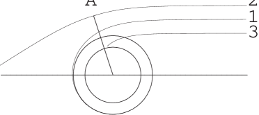
Figure 1: The above figure shows qualitatively the different types of motion for light rays in a spherically symmetric black hole background. Line 2 shows a ray which has a turning point, A. It corresponds to the scattering problem, that is when the ray coming from infinity is directly scattered back to infinity. Ray 1 corresponds to a critical trajectory when an incoming photon spirals around the circle (the critical radius) an infinite number of times. Ray 3 describes a motion of a photon coming from infinity which is captured by the black hole.

Similarly, the time of arrival of a forward emitted photons as measured by an observer at radius $r_{1}$ is

$$t^{(o)}_{+}=t^{(e)}_{+}+\int^{r_{1}}_{r_{0}}\frac{dr}{f\,Z}\,.$$ (12)

The integral in (12) is divergent when the upper limit tends to infinity. This divergence reflects a simple fact: namely, the time required for a light ray to reach infinity is infinitely large. For this reason it is more convenient to deal with the retarded time

$$u=t-\hat{r}\,\quad d\hat{r}={dr\over f}\,.$$ (13)

After simple transformations one has

$$u^{(o)}_{+}=u^{(e)}_{+}+T(r_{0})\,,$$ (14)

$$T(r_{0})=\int^{\infty}_{r_{0}}\,\frac{dr}{f}\left({1\over Z}-1\right)\,,$$ (15)

$$u^{(o)}_{-}=u^{(e)}_{-}+2(\hat{r}_{0}-\hat{r}_{*})+2T(r_{*})-T(r_{0})\,,$$ (16)

where $\hat{r}_{0}$ and $\hat{r}_{*}$ are tortoise–like coordinates, (13), for the point of emission and turning point, respectively.

In what follows we focus on the functions $\Phi$ and $T$ since the bending angle and retarded time for both forward and backward emitted photons can be expressed in terms of these quantities.

In the 4 dimensional spacetime, $n=1$, the integrals $(10)$ and $(15)$ can be written in terms of elliptic functions. In the higher dimensional case the integrals cannot be written in terms of known special functions. Our aim is to study these objects in a spacetime with arbitrary number of dimensions as functions of two variables, the impact parameter $\lambda$ specifying the photon trajectory, and the point of emission, $r_{0}$. It should be emphasized that knowledge of these scattering data allows one to obtain expressions for other quantities which might be of interest. For example, if one wants to know what are the bending angle and retarded time delay for a photon with given impact parameter propagating from one point, $r_{0}$, to another, $r_{1}$, it is sufficient to calculate the differences between the corresponding quantities $\Delta\phi_{\lambda}(r_{1})-\Delta\phi_{\lambda}(r_{0})$ and $\Delta u_{\lambda}(r_{1})-\Delta u_{\lambda}(r_{0})$.

II.2 The equations of motion in a dimensionless form

The problem contains only one dimensional parameter $r_{g}$, which determines the scale. It is convenient to introduce dimensionless quantities

$$q\equiv\frac{r_{g}}{r}\,,\quad q_{0}\equiv\frac{r_{g}}{r_{0}}\,,\quad l=\frac{\lambda}{r_{g}}\,.$$ (17)

In these variables

$$f=1-q^{n}\,,\quad Z=\sqrt{1-l^{2}q^{2}\,f}\,.$$ (18)

The motion of the photon is possible only in the region where

$$0\leq l\leq l_{max}={1\over q\sqrt{1-q^{n}}}\,.$$ (19)

(Notice that we consider only non-negative impact parameters.) On a plot in $(q,l)$ variables this region lies below the line $l_{max}(q)$. The allowed regions for different number of dimensions ($n\geq 1$) are similar. Figure 2 shows the allowed domain for $n=1$. The minimum of the function $l_{max}(q)$ is at $q=q_{*}$, where

$$q_{*}=\left({2\over n+2}\right)^{1/n}.\$$ (20)

At this point $l=l_{*}$ and $f=f_{*}$ where

$$l_{*}=\sqrt{{n+2\over n}}\left({n+2\over 2}\right)^{1\over n}\,,\hskip 14.22636ptf_{*}={n\over n+2}\,.$$ (21)

Before going further we distinguish the possible qualitatively different types of the light ray trajectories (see Fig. 2). Rays with $l<l_{*}$ can propagate from infinity ($q=0$) to the horizon ($q=1$) or travel to infinity from a point $q$ satisfying $q<1$. Rays with $l=l_{*}$ can either approach $q=q_{*}$ coming from the black hole ($q>q_{*}$) or from infinity $q=0$). In doing so they spiral around $q=q_{*}$ an infinite number of times. Rays with $l>l_{*}$ have a turning point. They can either propagate from infinity to some periastron and return to infinity or from the black hole horizon to an apastron and after fall back to the black hole. The latter case is not of much interest for astrophysical and other applications and we shall not consider it.

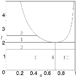
Figure 2: Function $l_{max}(q)$. Motion of photons is allowed in the region below this curve. Points $q=0$ and $q=1$ correspond to the infinity and the horizon, respectively. Horizontal lines describe the photon trajectories. Line 2 corresponds to a photon scattering, while line 3 corresponds to the photon capture. Line 1 is critical. It corresponds to a photon with the critical impact parameter $l_{*}$. Domain $I$ is a region below $=l_{max}(q)$ lying to the left from a vertical line 4. A region to the right from line 4 and below line 1 is domain $II$. In what follows we consider only photons emitted from domains $I$ and $II$, which can reach the infinity.

Using the above introduced dimensionless quantities we can rewrite the expressions for the bending angle and time delay in the following form

$$\Phi=\int_{0}^{q_{0}}{l\,dq\over Z(q)}\,,$$ (22)

$$T=r_{g}\int_{0}^{q_{0}}\frac{dq}{q^{2}f}\left({1\over Z(q)}-1\right)\,,$$ (23)

$$Z^{2}(q)=1-l^{2}q^{2}(1-q^{n})\,.$$ (24)

Let us consider the function $Z(q)$ in the interval from $q=0$ (infinity) to $q=1$ (horizon). It monotonically decreases from its value 1 at $q=0$ until the minimum

$$Z_{*}=\sqrt{1-(l/l_{*})^{2}}\,$$ (25)

at $q=q_{*}$, and then monotonically increases until it has the value 1 at $q=1$. It means that one can expect that for the integrals in (22) and (23) the main contribution comes either from the region near the point $q_{*}$ if it enters the integration domain, $q_{*}\in(0,q_{0})$, or from the region near the end point $q_{0}$ in the opposite case. We use this remark to construct an approximation for these integrals.

III Approximating the bending angle

III.1 Type $I$ rays

III.1.1 Leading part

First we study the rays emitted from the domain $I$ (type $I$ rays). Let us introduce a new coordinate $y$ related to $r$ and $q$ as follows

$$y=1-r_{0}/r\,,\hskip 14.22636ptq=q_{0}(1-y)\,,$$ (26)

and denote

$$p_{0} \equiv q_{0}/q_{*}\,,\hskip 5.69046ptp\equiv q/q_{*}=p_{0}(1-y)\,,\hskip 5.69046pt\,,$$ (27)

$$P = p_{0}^{n}\,,\hskip 5.69046ptB=\nu^{2}\,,\hskip 14.22636pt\nu\equiv l/l_{max}\,.$$ (28)

By fixing the parameters $P$ and $B$ one uniquely specifies a ray and its emission point. For the rays of type $I$ one has $0\leq P\leq 1$ and $0\leq B\leq 1$.

Using these notations one gets

$$f=1-{2P\over n+2}(1-y)^{n}\,,$$ (29)

and the expression for the bending angle for the forward emitted photons takes the form

$$\Phi = \int^{1}_{0}\frac{\nu\,dy}{Q}\,,$$ (30)

$$Q = \sqrt{f_{0}}Z=\sqrt{f_{0}-\nu^{2}(1-y)^{2}\,f}\,.$$ (31)

One also has

$$Q^{2}|_{y=0} = (1-B)(1-{2P\over n+2})\,,$$ (32)

$$Q^{2}|_{y=1} = f_{0}=1-2P/(n+2)\,.$$ (33)

We study now $\Phi$ as a function of $(P,B)$ in the domain $I:$  $0\leq P,B\leq 1$. Our goal is to obtain an analytic expression uniformly approximating $\Phi$ in this region.

For the interval $(0,q_{0}\leq q_{*})$ in the domain $I$ the function $Q$ has its minimal values at $y=0$ which corresponds to $q=q_{0}$. We denote by $\hat{Q}^{2}$ the expansion of $Q^{2}$ in $y$ up to the second order

$$\hat{Q}^{2} = a+2by+cy^{2}\,,$$ (34)

$$a = (1-B)(1-{2P\over n+2})\,,$$

$$b = B(1-P)\,,$$ (35)

$$c = -B[1-(n+1)P]\,.$$

In the domain $I$ the parameters $a$ and $b$ are always positive, while $c>0$ for $P>1/(n+1)$ and $c<0$ for $P<1/(n+1)$. At the point $y=0$, $\hat{Q}^{2}$ and its first two derivatives coincide with the similar quantities for the function $Q^{2}$. In particular, at in the vicinity of the point $(P=B=1)$ one has

$$Q\sim\hat{Q}\sim\sqrt{n}y+\ldots\,.$$ (36)

At the point $y=1$ one has

$$A\equiv\hat{Q}^{2}|_{y=1}=1-{2P\over n+2}+{n(n+1)\over n+2}BP\,.$$ (37)

Let us denote

$$\hat{\Phi}=\int^{1}_{0}\frac{\nu\,dy}{\hat{Q}}\,,$$ (38)

and present $\Phi$ in the form

$$\Phi=\hat{\Phi}+\Delta{\Phi}\,.$$ (39)

Both integrals, $\Phi$ and $\hat{\Phi}$ are logarithmically divergent at the lower limit, $y=0$, for the point $P=B=1$ of the parameter space. This point corresponds to a trajectory with the impact parameter $l=l_{*}$ emitted at $q=q_{*}$. As a consequence of the property (36) the divergences of the both quantities $\Phi$ and $\hat{\Phi}$ are identical and hence $\Delta\Phi$ remains finite at $P=B=1$. The integral (38) can be easily taken. We shall discuss now its exact value and later we shall find a suitable approximation for $\Delta{\Phi}$ valid in the total domain $I$.

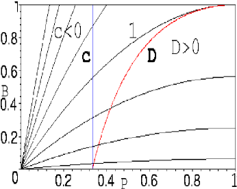
Figure 3: The above figure shows the domain $I$ of Figure 2 in $(P,B)$ coordinates. The line 1 originating from the point $(0,0)$ and terminating at the point $(1,1)$ corresponds to photons with the critical value of the impact parameter. Lines originating from the point $(0,0)$ which are above line 1 correspond to line 2 in figure 2 and lines below it correspond to line 3 in figure 2. The line $\bf c$ where $P=1/(n+1)$, separates two regions where $c<0$ (to the left) and $c>0$ (to the right). The discriminant $D$ vanishes on the line ${\bf D}$. A region with negative $D$ is to the left of this line, and the region with positive $D$ is to the right of the line ${\bf D}$. The plot is shown for $n=2$. For other values of $n$ the structure is similar.

The form of the expression for $\hat{\Phi}$ depends on the sign of c and on the sign of the discriminant $D$ (see figure 3),

$$D=ac-b^{2}\,.$$ (40)

The equation of the line where $D=0$ is

$$B=[(n+1)P-1](n+2-2P)/(nP(n+1-P))\,.$$ (41)

This line is shown in Fig. 3. It starts at $B=0$ and $P=1/(n+1)$ and ends at the corner $P=B=1$. The vertical lines in the figure 3 correspond to the fixed value of $P$ (and hence of $q$ and $r$). The lines which start at the point $(0,0)$ in this figure correspond to the fixed values of the impact parameter $l$ and are described by the equation

$$B=l^{2}q_{*}^{2}P^{2/n}[1-2P/(n+2)]\,.$$ (42)

Inside the domain $I$ for $c<0$ one has $D<0$ and

$$\hat{\Phi}=\frac{\nu}{\sqrt{{-c}}}\arcsin\left({\sqrt{{-c}}B\over{D}}[nP\sqrt{a}-(1-P)\sqrt{A}]\right)\,.$$ (43)

The parameters $A$ and $D$ which enter this relation are defined by (37) and (40), respectively.

Taking the limit $c\to 0$, $(B\neq 0)$, in this expression one obtains

$$\hat{\Phi}=\frac{\nu}{b}(\sqrt{a+2b}-\sqrt{a})\,.$$ (44)

Finally for $c>0$ one has

$$\hat{\Phi}=\frac{\nu}{\sqrt{c}}\ln{\left(\frac{nBP+\sqrt{cA}}{b+\sqrt{ac}}\right)}\,.$$ (45)

We shall need later the expression of $\hat{\Phi}$ for the special value $P=1$. In this case $c>0$. We denote this quantity by $\hat{\Phi}_{*}$. For this choice one has $q_{0}=q_{*}$, $l_{max}=l_{*}$ and $\nu$ takes the value $\mu=l/l_{*}$. Taking this limit in the formula (45) one obtains

$$\hat{\Phi}_{*}={1\over\sqrt{n}}\ln\left[{\mu\sqrt{n+2}+\sqrt{(n+2)\mu^{2}+1-\mu^{2}}\over\sqrt{1-\mu^{2}}}\right]\,.$$ (46)

For a trajectory close to the critical one, $\mu\approx 1$,

$$\hat{\Phi}_{*}\sim-{1\over 2\sqrt{n}}\ln{(1-\mu)}\,.$$ (47)

III.1.2 Approximating $\Delta\Phi$

Figure 4: This is a plot for $n=2$ of the surface $\Delta{\Phi}$ for rays in domain $I$ when it is rotated to have an orientation [-47^∘, 90^∘]

Now we focus our attention on the quantity $\Delta{\Phi}$ which describes the difference between the exact value of the bending angle $\Phi$ and its leading part $\hat{\Phi}$ which we calculated in the previous subsection. We have plotted $\Delta{\Phi}$ as a function of $p_{0}$ and $\nu$ in the domain $I$. After a study of these plots we found a remarkable fact. Namely, $\Delta{\Phi}$, which by its definition is a function of 2 variables, $P$ and $B$, can be approximated accurately enough by a function of one variable, which is a linear combination of $p_{0}$ and $\nu$. We found that this fact is valid not only in 4 dimensions, but in higher dimensions as well. Figure 4 illustrates this. It gives an example of the 3D plot of $\Delta\Phi$ constructed by ${\it Maple}$ for $n=2$ ($D=5$) with the orientation option for the view angles chosen to be $[-47^{\circ},90^{\circ}]$. The 2D surface in this projection is a slightly broadened curve. Similar orientation angles can be found for other dimensions. Using this fact and by fitting the corresponding 2D plots, one can find the following expression which approximate $\Delta\Phi$ with a very high accuracy

$$\Delta\hat{\Phi} = -k_{\Phi}(\sqrt{1-(x_{\Phi}-1)^{2}}-1)\Theta(x_{\Phi}-1)\,,$$ (48)

$$x_{\Phi} = \sqrt{2}[\cos(\frac{\pi}{4}+\psi_{\Phi})p_{0}+\sin(\frac{\pi}{4}+\psi_{\Phi})\nu]\,.$$ (49)

Here $\Theta$ is the Heaviside step function. The parameters $k_{\Phi}$ and ${\psi}_{\Phi}$ for different number of spacetime dimensions are given in Table 1.

Dimension	$k_{\Phi}$	$\psi_{\Phi}$	Percentage error $\delta_{\Phi}$
D=4,n=1	$0.47$	$\pi/45$	[-0.77% , 1.78%]
D=5,n=2	$0.49$	$\pi/90$	[-1.20% , 1.69%]
D=6,n=3	$0.52$	$0$	[-2.10% , 1.71%]
D=7,n=4	$0.55$	$0$	[-2.89% , 2.58%]

Table 1: Approximation parameters $k_{\Phi}$ and $\psi_{\Phi}$, and range of relative errors $\delta_{\Phi}$ for $\Phi$ in the domain $I$ for the spacetime of dimension $D=n+3$.

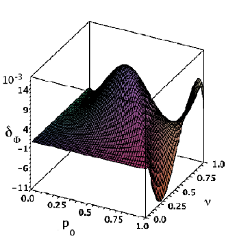
Figure 5: This is a plot for $n=2$ of the surface $\delta_{\Phi}$ for rays in domain $I$ when rotated to haave the orientation [-70^∘, 64^∘].

This observation implies that one can approximate $\Phi$ by the following expression

$$\Phi\approx\Phi^{a}=\hat{\Phi}+\Delta\hat{\Phi}\,.$$ (50)

Here $\hat{\Phi}$ is given by (43)-(45), and $\Delta\hat{\Phi}$ is given by (48)-(49). The relative error of this approximation is

$$\delta_{\Phi}={\Phi-\Phi^{a}\over\Phi}={\Delta\Phi-\Delta\hat{\Phi}\over\Phi}\,.$$ (51)

Such a relative error calculated in the domain $I$ belongs to some error interval. These error intervals for the spacetimes with different number of dimensions are given in Table 1. The figure 5 illustrates how the relative error $\delta_{\Phi}$ is distributed in the space of parameters $(p_{0},\nu)$. This particular plot of the surface $\delta_{\Phi}$ is again shown for $n=2$. The plots for other values of $n$ are similar. It is evident from the figure that our approximation for the bending angle works very well everywhere in the domain $I$ including the region near $(p_{0}=1,\nu=1)$ which is precisely where the integral expression for the bending angle diverges.

III.2 Type $II$ rays

III.2.1 Leading part

For the light ray emitted from the domain $II$ the main contribution to the bending angle is from an interior point of the integration domain. For this reason the above procedure for obtaining the analytical approximation for the bending angle must be slightly modified. We rewrite the expression (22) for the bending angle in the form

$$\Phi=\mu\sqrt{n+2\over n}\int_{0}^{p_{0}}{dp\over Z(p)}\,,$$ (52)

where, as earlier $p=q/q_{*}$, $\mu=l/l_{*}$ and

$$Z^{2}(p)=1-{n+2\over n}\mu^{2}p^{2}(1-{2\over n+2}p^{n})\,.$$ (53)

Since $p_{0}>1$ and the function $Z(p)$ has its minimum at $p=1$, it is convenient to split the integration domain in (52) into intervals $(0,1)$ and $(1,p_{0})$. To approximate the first integral

$$\Phi_{*}=\mu\sqrt{n+2\over n}\int_{0}^{1}{dp\over Z(p)}$$ (54)

one can use the expression obtained in the previous section

$$\Phi_{*}\approx\hat{\Phi}_{*}+\Delta\hat{\Phi}_{*}\,,$$ (55)

where $\hat{\Phi}_{*}$ is given by (46), while $\Delta\hat{\Phi}_{*}$ is $\Delta\hat{\Phi}$, given by (48), calculated for $p_{0}=1$. Thus, for our purposes, it is sufficient to discuss the approximation of the following quantity

$$\Phi_{II}=\mu\sqrt{n+2\over n}\int_{1}^{p_{0}}{dp\over Z(p)}\,.$$ (56)

Expanding the function $Z^{2}(p)$ in the powers of $(p-1)$ near its minimum, $p-1=0$, and keeping the terms up to the second order one obtains

$$\hat{Z}^{2}=(1-\mu^{2})+(n+2)\mu^{2}(p-1)^{2}\,.$$ (57)

As earlier, we substitute $\hat{Z}(p)$ instead of $Z(p)$ in (56)

$$\hat{\Phi}_{II}=\mu\sqrt{n+2\over n}\int_{1}^{p_{0}}{dp\over\hat{Z}(p)}\,.$$ (58)

This integral can be taken explicitly and defining $z=\mu\sqrt{n+2}(p_{0}-1)$ one gets

$$\hat{\Phi}_{II} = {1\over\sqrt{n}}\ln{z+\sqrt{z^{2}+1-\mu^{2}}\over\sqrt{1-\mu^{2}}}\,.$$ (59)

We now turn our attention to the relative error in the approximation of $\Phi_{II}$ by $\hat{\Phi}_{II}$. The relative error is

$$\delta^{\Phi}_{II}={\Phi_{II}-\hat{\Phi}_{II}\over\Phi_{II}}={\Delta{\Phi}_{II}\over\Phi_{II}}\,.$$ (60)

The relative errors in the dimensions considered are given in Table II and the figure 6 is a plot of $\delta^{\Phi}_{II}$ in five dimensions, the plots for other dimensions are similar. One can improve the accuracy of the approximation for $\Phi_{II}$ as it was done for rays emitted in the domain $I$. However, for most of our purposes it is sufficient to approximate $\Phi_{II}$ by $\hat{\Phi}_{II}$. This happens because the relative contribution to the bending angle by the inner part of the ray lying within the domain $II$, $(1>q>q_{*})$, is smaller than the contribution from the part of this ray in the domain $I$. For this reason the contribution to the ‘inaccuracy’ of the inner part to the total ‘inaccuracy’ is suppressed. This can be seen from the Table II which contains both relative errors, $\delta_{\Phi}$ and $\delta^{\Phi}_{II}$. Thus for the approximation of the inner contribution $\Phi_{II}$ to the bending angle it is sufficient to use only the leading term $\hat{\Phi}_{II}$.

Using this information we approximate the bending angle for light propagating to infinity from domain $II$ by

$$\Phi^{a}=\hat{\Phi}_{*}+\Delta\hat{\Phi}_{*}+\hat{\Phi}_{II}\,.$$ (61)

The use of our approximation in the previous section and $\hat{\Phi}_{II}$ accounts for the reasonably good relative error of our approximation of the bending angle for light coming from domain $II$. The relative error of our approximation is

$$\delta_{\Phi}={\Phi-\Phi^{a}\over\Phi}\,.$$ (62)

The Table $II$ contains the relative errors appropriate to each value of $n$ considered. The figure 7 is a plot of $\delta_{\Phi}$ for $n=2$. We can see that our approximation remains good in the region where the bending angle diverges.

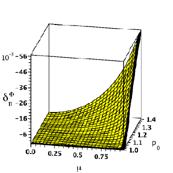
Figure 6: This is a plot for $n=2$ of the surface $\delta^{\Phi}_{II}$ for rays in domain $II$ for $p_{0}$ satisfying $1\leq p_{0}\leq 1.41$, $0\leq\mu\leq 0.99$ when it is rotated to have an orientation [-9^∘, -107^∘]. We don’t show the region for $0.99\leq\mu\leq 1$ because the plot descends steeply to zero in this region and it is difficult to show the nature of the plot of this region on this scale.

Dimension	$p_{0}$	Percentage error $\delta^{\Phi}_{II}$	Percentage error $\delta_{\Phi}$
D=4,n=1	$p_{0}=1.49$	[-4.38%, 0.00%]	[-1.30%, 0.83%]
D=5,n=2	$p_{0}=1.41$	[-5.69%, 0.00%]	[-1.80% , 1.15%]
D=6,n=3	$p_{0}=1.35$	[-6.64%, 0.00%]	[-2.11% , 1.72%]
D=7,n=4	$p_{0}=1.31$	[-7.50%, 0.00%]	[-2.25% , 2.56%]

Table 2: Above are the relative errors associated with the quantities $\delta^{\Phi}_{II}$ and $\delta_{\Phi}$ for $\Phi_{II}$ and $\Phi$ in the domain $II$ for $p_{0}$ satisfying $1\leq p_{0}\leq q^{-1}_{*}$ for the spacetimes of dimension $D=n+3$. Also included are the maximal values of $p_{0}$ considered for the endpoint of integration.

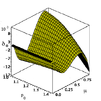
Figure 7: This is a plot for $n=2$ of the surface $\delta_{\Phi_{II}}$ for rays in domain $II$ for $p_{0}$ satisfying $1\leq p_{0}\leq 1.41$,$0\leq\mu\leq 0.99$ when it is rotated to have an orientation [-48^∘, 62^∘]. We don’t show the region for $0.99\leq\mu\leq 1$ because the plot descends steeply to zero in this region and it is difficult to show the nature of the plot of this region on this scale.

IV Approximating the time delay

IV.1 Type $I$ rays

IV.1.1 Leading part

The time delay $t^{(o)}-t^{(e)}$, (12), and the corresponding delay in the retarded time $u$, (14), is defined by the function $T$, (15), or its dimensionless form $\tau$

$$T=r_{g}q^{-1}_{0}\tau\,,\hskip 14.22636pt\tau=\int^{1}_{0}\frac{dy}{(1-y)^{2}\,f}\left({\sqrt{f_{0}}\over Q}-1\right)\,.$$ (63)

We now construct an analytic approximation for $\tau$ in the same way as it was done for $\Phi$ in the previous section. It is easy to see that in spite of the factor $(1-y)^{2}$ in the denominator of the integrand in (63), the integral is finite at $y=1$. The only singular point of $\tau$ in the domain $I$ is its logarithmic divergence at $y=0$ for the limiting values of the parameters $p_{0}=\nu=1$. To extract this divergence we subtract from $\tau$ a similar integral, where instead of $Q$ we use $\hat{Q}$ given by (34). In order to be able to obtain the value of the integral in an explicit form in terms of elementary functions, as earlier, we make another modification of the integrand. Namely, instead of $H=(1-y)^{2}f$ we use its quadratic expansion near $y=0$ of the form

$$\hat{H} = f_{0}+2\beta y+\gamma y^{2}\,$$ (64)

$$f_{0} = 1-{2P\over n+2}\,,\quad\beta=-(1-P)\,,$$ (65)

$$\gamma = 1-(n+1)P\,,\hskip 5.69046ptP=p_{0}^{n}\,.$$ (66)

It is easy to see that $f_{0}\geq 0$ and that the discriminant of the quadratic in $y$, (64), is of the form

$$f_{0}\gamma-\beta^{2}=-{nP(n+1-P)\over n+2}={D-f_{0}c\over\nu^{4}}\,$$ (67)

and is non-positive. The parameters $a$, $b$, and $c$, which enter the expression $\hat{Q}$, (34), are related to the coefficients in (64) as follows

$$a=(1-\nu^{2})f_{0}\,,\hskip 5.69046ptb=-\nu^{2}\beta\,,\hskip 5.69046ptc=-\nu^{2}\gamma\,.$$ (68)

Let us emphasize that the structure of the logarithmic divergence of the exact integral (63) at $y=0$ is preserved in our approximation since $\hat{H}(y=0)=f_{0}=[(1-y)^{2}f]|_{y=0}$.

We define the quantity $\hat{\tau}$ as follows

$$\hat{\tau}=\int^{1}_{0}\frac{dy}{\hat{H}}\left({\sqrt{f_{0}}\over\hat{Q}}-1\right)\,.$$ (69)

We note that $\hat{H}$ has a root in the interval $[0,1]$. Rewriting the integrand in (69) as follows

$$\frac{1}{\hat{H}}\left({\sqrt{f_{0}}\over\hat{Q}}-1\right)=\frac{\nu^{2}}{\sqrt{f_{0}}\hat{Q}+\hat{Q}^{2}}\,,$$ (70)

one can see that it does not result in a divergence. Defining the following quantities:

$$M = f_{0}c-D\,,$$

$$\cal{A}_{\pm} = D+c\sqrt{f_{0}A}\pm\,(c+b)\sqrt{M}\,,$$ (71)

$$\cal{B}_{\pm} = D+c\sqrt{f_{0}a}\pm\,b\sqrt{M}\,,$$

where, as earlier, $D=ac-b^{2}$, the explicit form of $\hat{\tau}$ is

$$\hat{\tau} = \frac{\nu^{2}}{2\sqrt{M}}\ln{\left(\frac{{\cal A}_{+}{\cal B}_{-}}{{\cal A}_{-}{\cal B}_{+}}\right)}.$$ (72)

In the case $c=0$, $(B\neq 0)$, $\hat{\tau}$ has the following form

$$\hat{\tau} = \frac{\nu^{2}}{2b}\ln{\left(\frac{a+2b-f_{0}}{a-f_{0}}\right)}\,$$ (73)

$$+ \frac{\nu^{2}}{b}\tanh^{-1}\left(\frac{\sqrt{f_{0}}(\sqrt{a+2b}-\sqrt{a})}{f_{0}-\sqrt{a}\sqrt{a+2b}}\right)\,.$$

For the boundary of the domain $I$ where $q=q_{*}$ ($p_{0}=1$) the expression for $\hat{\tau}$ simplifies and takes the form

$$\hat{\tau}_{*} = {\sqrt{n+2}\over 2n}\ln{(Z_{+}/Z_{-})}\,,$$ (74)

$$Z_{\pm} = Bn\sqrt{n+2}\pm(n-nB+n\sqrt{(n+1)B+1})\,.$$

For the near critical rays ($\mu-1\approx 0$)

$$\hat{\tau}_{*}\sim{\sqrt{n+2}\over 2n}\left[-\ln(\mu-1)+\ln\left({{n+2}\over 2\sqrt{n+2}+n+3}\right)\right]+\ldots\,.$$ (75)

This time is logarithmically divergent at $\mu\to 1$.

As in the case for $\Phi$ we can express the quantity $\tau$ as

$$\tau=\hat{\tau}+\Delta\tau\,,$$ (76)

the quantity $\Delta\tau$ being finite for rays moving along critical trajectories.

IV.1.2 Approximating $\Delta\tau$

Figure 8: This is a plot for $n=2$ of the surface $\Delta{\tau}$ when it is rotated to have an orientation [-45^∘, 90^∘]. We note that we use the orientation [-43^∘, 90^∘] in our approximation because it better approximates a curve.

As earlier, by studying of the plots for $\Delta{\tau}$ as a function of 2 variables $p_{0}$ and $\nu$ one can observe that they can be approximated by a function of one variable, which is a linear combination of $p_{0}$ and $\nu$. For example, figure 8 shows the 3D plot of $\Delta\tau$ for $n=2$ ($D=5$) with the orientation option chosen to be $[-43^{\circ},90^{\circ}]$. The 2D surface in this projection is again a slightly broadened curve. This allows one to approximate $\Delta\tau$ with a very good accuracy by a function

$$\Delta{\hat{\tau}}=-k_{\tau}p_{0}\nu(\sqrt{1-(x_{\tau}-1)^{2}}-1)\Theta(x_{\tau}-1)\,,$$ (77)

$$x_{\tau}=\sqrt{2}[\cos(\frac{\pi}{4}+\psi_{\tau})p_{0}+\sin(\frac{\pi}{4}+\psi_{\tau})\nu]\,.$$ (78)

The corresponding values of $k_{\tau}$ and $\psi_{\tau}$ are given in Table 3. Thus we can approximate $\tau$ as follows

$$\tau\approx\tau^{a}=\hat{\tau}+\Delta{\hat{\tau}}\,.$$ (79)

Dimension	$k_{\tau}$	$\psi_{\tau}$	Percentage error $\delta_{\tau}$
D=4,n=1	$0.66$	$\pi/45$	[-1.68% , 2.71%]
D=5,n=2	$0.55$	$\pi/90$	[-2.19% , 2.60%]
D=6,n=3	$0.52$	$0$	[-3.28% , 2.31%]
D=7,n=4	$0.52$	$\pi/60$	[-1.73% , 2.66%]

Table 3: Approximation parameters $k_{\tau}$ and $\psi_{\tau}$, and range of relative errors $\delta_{\tau}$ for $\tau$ in the domain $II$ for the spacetime of dimension $D=n+3$.

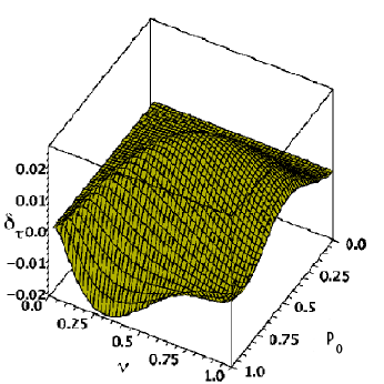
Figure 9: This is a plot for $n=2$ of the surface $\delta_{\tau}$ when it is rotated to have an orientation [29^∘, 46^∘]

The figure 9 is a plot of the surface $\delta_{\tau}$ for the domain $I$, $0\leq\{p_{0},\nu\}\leq 1$. Here we have shown $\delta_{\tau}$ for $n=2$. The plots for other values of $n$ are similar. The relative error of this approximation is

$$\delta_{\tau}={\tau-\tau^{a}\over\tau}={\Delta\tau-\Delta{\hat{\tau}}\over\tau}\,.$$ (80)

The relative errors $\delta_{\tau}$ for a spacetime with different number of dimensions are given in Table 3. It is evident from the figure that our approximation for the time delay works very well in the region near $(p_{0}=1,\nu=1)$ which is precisely where the integral expression for the retarded time diverges.

IV.2 Type $II$ rays

IV.2.1 Leading part

In this section we investigate the retarded time for light rays that proceed to infinity from the domain $II$ where $p_{0}$ satisfies $1\leq p_{0}<((n+2)/2)^{1/n}$. As in the case of type $I$ rays we express the retarded time for a light ray emitted in domain $II$ in terms of dimensionless quantities. In this instance we use the quantities $p_{0}$ and $\mu$ as defined earlier. After reformulating the expression for the retarded time, (15), in terms of these variables we have

$$T=r_{g}q_{*}^{-1}\tau\,,\hskip 5.69046pt\tau=\mu^{2}\left(1+{2\over n}\right)J(0,p_{0})\,,$$ (81)

$$J(p_{1},p_{0})=\int^{p_{0}}_{p_{1}}\frac{{dp}}{Z(p)(1+Z(p))}\,.$$ (82)

Since we are in a region where $p_{0}>1$ and $Z(p)$ has a minimum at $p=1$ we again split the integration domain in $(\ref{jj})$ into two intervals, $(0,1)$ and $(1,p_{0})$. In the first interval we can write the contribution to the retarded time as

$$\tau_{*}=\mu^{2}\left(1+{2\over n}\right)J(0,1)\,.$$ (83)

This integral can be approximated by

$$\tau_{*}\approx\hat{\tau}_{*}+\Delta\hat{\tau}_{*}\,,$$ (84)

where $\hat{\tau}_{*}$ is given by $(\ref{www})$ and $\Delta\hat{\tau}_{*}$ is $\Delta\hat{\tau}$ evaluated at $p_{0}=1$. Therefore in approximating the retarded time in domain $II$ it is sufficient for our purposes to consider the following integral

$$\tau_{II}=\mu^{2}\left(1+{2\over n}\right)J(1,p_{0})\,.$$ (85)

Identically to what we did earlier we substitute $\hat{Z}(p)$ given by (57) for $Z(p)$ to obtain

$$\hat{\tau}_{II}=\mu^{2}\left(1+{2\over n}\right)\hat{J}(1,p_{0})\,,$$ (86)

$$\hat{J}(1,p_{0})=\int^{p_{0}}_{p_{1}}\frac{{dp}}{\hat{Z}(p)(1+\hat{Z}(p))}\,.$$ (87)

This integral is calculated explicitly using Maple and is given by

$$\hat{\tau}_{II}=\frac{\sqrt{n+2}}{2n}\ln{\frac{\sqrt{1-\mu^{2}+z^{2}}+1-\mu^{2}+\mu z}{\sqrt{1-\mu^{2}+z^{2}}+1-\mu^{2}-\mu z}}\,.$$ (88)

We now focus our attention on the relative error $\delta^{\tau}_{II}$

$$\delta^{\tau}_{II}={\tau_{II}-\hat{\tau}_{II}\over\tau_{II}}={\Delta\hat{\tau}_{II}\over\tau_{II}}\,$$ (89)

of the approximation of $\tau_{II}$ by $\hat{\tau}_{II}$. In Table IV we present the relative errors of our first order approximation of $\tau_{II}$ for dimensions $4,5,6,7$. The figure 10 is a plot of $\delta^{\tau}_{II}$ in five dimensions, the plots in other dimensions are similar. As earlier, examining the results presented in Table IV we can conclude that $\hat{\tau}_{II}$ provides a good first order approximation of the function $\tau_{II}$ in the domain $II$. Therefore in approximating the retarded time for light going to infinity from domain II we use

$$\tau^{a}=\hat{\tau}_{*}+\Delta\hat{\tau}_{*}+\hat{\tau}_{II}\,,$$ (90)

and the corresponding relative error of our approximation for the retarded time delay is

$$\delta_{\tau}={\tau-\tau^{a}\over\tau}\,.$$ (91)

This relative error for each dimension considered is shown in Table IV. The figure 11 is a plot of $\delta_{\tau}$ for $n=2$. We can see that our approximation is very good in the region $\mu\sim 1$, which is where the retarded time diverges.

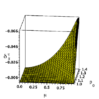
Figure 10: This is a plot for $n=2$ of the surface $\delta^{\tau}_{II}$ in domain $II$ for $p_{0}$ satisfying $1\leq p_{0}\leq 1.41$, $0\leq\mu\leq 0.99$ when it is rotated to have an orientation [-6^∘, -106^∘]. We don’t show the region for $0.99\leq\mu\leq 1$ because the plot descends steeply to zero in this region and it is difficult to show the nature of the plot of this region on this scale.

Dimension	$p_{0}$	Percentage error $\delta^{\tau}_{II}$	Percentage error $\delta_{\tau}$
D=4,n=1	$p_{0}=1.49$	[-5.18%, 0.00%]	[-2.00%, 0.72%]
D=5,n=2	$p_{0}=1.41$	[-6.73%, 0.00%]	[-2.52%, 0.16%]
D=6,n=3	$p_{0}=1.35$	[-7.83%, 0.00%]	[-3.24%, 0.67%]
D=7,n=4	$p_{0}=1.31$	[-8.83%, 0.00%]	[-2.59%, 2.67%]

Table 4: This table shows the relative errors associated with the quantities $\delta^{\tau}_{II}$ and $\delta_{\tau}$ for our approximation of $\tau_{II}$ and $\tau$ in the domain $II$ for $p_{0}$ satisfying $1\leq p_{0}\leq q^{-1}_{*}$ for the spacetimes of dimension $D=n+3$. Also included are the maximal values of $p_{0}$ considered for the endpoint of integration.

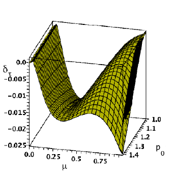
Figure 11: This is a plot for $n=2$ of the surface $\delta_{\tau}$ for rays in domain $II$ for $p_{0}$ satisfying $1\leq p_{0}\leq 1.41$,$0\leq\mu\leq 0.99$ when it is rotated to have an orientation [14^∘, 67^∘]. We don’t show the region for $0.99\leq\mu\leq 1$ because the plot descends steeply to zero in this region and it is difficult to show the nature of the plot of this region on this scale.

V Summary and Discussion

In the present paper we have investigated ray-tracing problem for photons propagating in four and higher dimensional spherically symmetric black hole backgrounds. We focused on the bending angle and the retarded time for a trajectory of the null ray with the impact parameter $\lambda$ which starts at some finite radius $r_{0}$ and propagates to the infinity. We obtained an analytical expression in terms of the elementary functions which uniformly approximate the bending angle $\Phi_{\lambda}(r_{0})$ and the retarded time function $T_{\lambda}(r_{0})$ with high accuracy. Knowledge of these two functions, $\Phi_{\lambda}(r_{0})$ and $T_{\lambda}(r_{0})$, allows one to calculate other quantities which are of interest in possible applications.

For example, let us consider a scattering problem, when a photon with a given impact parameter $\lambda$ comes from infinity and after passing near the black hole goes to infinity again. The total bending angle for this process is $2\Phi_{\lambda}(r^{*})$, where $r^{*}$ is the radius of the photon’s turning point. This quantity can be approximated by $2\hat{\Phi}_{*}$, where $\hat{\Phi}_{*}$ is given by (46). Similarly, the expression (74) can be used for an approximation of the time delay quantities for the scattering problem.

A knowledge of the bending angle function $\Phi_{\lambda}(r)$ is sufficient for a reconstruction a complete ray trajectory. Really, let us fix the impact parameter $\lambda$ and consider a ray with this impact parameter emitted at the radius $r_{0}$ in the D-dimensional Schwarzschild-Tangherlini space. Since the ray trajectories are planar, it is sufficient to consider rays lying in the equatorial plane passing through the point of emission. We choose $\phi_{0}=0$ for this point. The ray trajectory is defined by the equation

$$\phi=F(r)=\Phi_{\lambda}(r)-\Phi_{\lambda}(r_{0})\,.$$ (92)

To obtain an approximated form of the trajectory equation it is sufficient to substitute $\Phi^{a}$ instead of the exact values $\Phi$.

Similarly one can use the approximating expression for solving the problem of the reconstruction of a null geodesic connecting two points $(r_{0},\phi_{0})$ and $(r_{1},\phi_{1})$. In the 4 dimensional case this problem can be reduced to one non-linear equation which contains as the arguments the Jacobi elliptic functions CaKo . By using the developed approximation one can reduce this problem in any number of dimensions to solving non-linear equations which contain only elementary functions.

We hope that the obtained results will be useful in studying these and other problems connected with light propagation in the black hole vicinity which are of interest in the application to astrophysics. Since the developed approximation is valid in a spacetime with arbitrary number of dimensions, it might be useful also for study black holes in the models with large extra dimensions.

References

- (1) Y. Tanaka et al., Nature (London) 375 659 (1995).
- (2) T. Yaqoob, I. M. George, T. J. Turner, K. Nandra, A. Ptak and P. J. Serlemitsos, ApJ 505 L87 (1998), arXiv:astro-ph/9807349.
- (3) Reynolds, C. S., Fabian, A. C., Nandra, K., Inoue, H., Kunieda, H., & Iwasawa, K., MNRAS 277, 901 (1995).
- (4) Turner, T. J., George, I. M., Nandra, K., & Mushotzky, R. F., ApJ 488, 164 (1997).
- (5) Nandra, K., George, I. M., Mushotzky, R. F., Turner, T. J., & Yaqoob, T., ApJ 477, 602 (1997).
- (6) Fanton, C., Calvani, M., de Felice, F., & Čadež, A., PASJ 49, 159 (1997).
- (7) Bromley, B. C., Chen, K., & Miller, W. A., ApJ 475, 57 (1997).
- (8) Dabrowski, Y., & Lasenby, A. N., MNRAS 321, 605 (2001).
- (9) Čadež, A., Fanton, C., & Calvani, M., New A 3, 647 (1998).
- (10) Martocchia, A., Karas, V., & Matt, G., MNRAS 312, 817 (2000).
- (11) Baganoff, F. K., Bautz, M. W., Brandt, W. N., Chartas, G., Feigelson, E. D., Garmire, G. P., Maeda, Y., Morris, M., Ricker, G. R., Townsley, L. K., & Walter, F., Nature (London) 413, 45 (2001).
- (12) Goldwurm, A., Brion, E., Goldoni, P., Ferrando, P., Daigne, F., Decourchelle, A., Warwick, R. S., & Predehl, P., ApJ 584, 751 (2003).
- (13) Strohmayer, T. E., ApJ 552 L49 (2001).
- (14) Miller, J. M., Fabian, A. C., Wijnands, R., Reynolds, C. S., Ehle, M., Freyberg, M. J., van der Klis, M., Lewin, W. H. G., Sanchez-Fernandez, C., & Castro-Tirado, A. J., ApJ 570, L69 (2002).
- (15) R. Emparan and H. S. Reall, Black Holes in Higher Dimensions, e-Print: arXiv:0801.3471 [hep-th] (2008).
- (16) B. Carter, Phys. Rev. 174, 1559 (1968).
- (17) C. Darwin, Proc. Roy. Soc. Lon. A 249, 180 (1959).
- (18) C. Darwin, Proc. Roy. Soc. Lon. A 263, 39 (1961).
- (19) G. V. Kraniotis, Class. Quant. Grav. 22, 4391, (2005).
- (20) V. P. Frolov, D. Kubizňák, Phys. Rev. Lett. 98, 011101 (2007).
- (21) D. Kubizňák, V. P. Frolov, Class. Quant. Grav. 24, F1 (2007).
- (22) P. Krtouš, D. Kubizňák, D. N. Page, and V. P. Frolov, JHEP 0702, 004 (2007).
- (23) P. Krtouš, D. Kubizňák, D. N. Page, M. Vasudevan, Phys. Rev. D 76, 084034 (2007).
- (24) D. N. Page, D. Kubizňák, M. Vasudevan, P. Krtouš, Phys. Rev. Lett 98, 061102 (2007).
- (25) V. P. Frolov, P. Krtouš, and D. Kubizňák, JHEP 0702, 005 (2007).
- (26) T. Oota, Y. Yasui, Phys. Lett. B 659, 688 (2008).
- (27) V. P. Frolov, Hidden Symmetries of Higher-Dimensional Black Hole Spacetimes, e-Print: arXiv:0712.4157 [gr-qc] (2007).
- (28) V. P. Frolov, D. Kubizňák, Higher-Dimensional Black Holes: Hidden Symmetries and Separation of Variables, e-Print: arXiv:0802.0322 [hep-th] (2008).
- (29) J. Briët and D. W. Hobill, Determining the Dimensionality of Spacetime by Gravitational Lensing, Preprint arXiv: 0801.3859 (2008).
- (30) C. Gooding and A. V. Frolov, Five-dimensional black hole capture cross-sections, Preprint arXiv: 0803.1031, (2008).
- (31) A. M. Beloborodov, Astrophys. J. 566, L85 (2002).
- (32) V. P. Frolov, H. K. Lee, Phys. Rev. D 71 044002 (2005).
- (33) V. R. Eshleman, E. M. Gurrola, and G. F. Lindal, Adv. Space Res., 9, No.9, 119 (1989).
- (34) V. Bozza, G. Scarpetta, Phys. Rev. D 76 083008 (2007).
- (35) A. Čadež and U. Kostić, Phys. Rev. D 72, 104024 (2005). [arXiv:gr-qc/0405037].