Slow Excitation Trapping in Quantum Transport with Long-Range Interactions

Abstract

Long-range interactions slow down the excitation trapping in quantum transport processes on a one-dimensional chain with traps at both ends. This is counter intuitive and in contrast to the corresponding classical processes with long-range interactions, which lead to faster excitation trapping. We give a pertubation theoretical explanation of this effect.

Building a quantum system from scratch has become possible due to recent experimental advances in controlling and manipulating atoms and molecules. It has actually become possible to tailor theoreticians favourite one-dimensional systems using, e.g., ultra-cold atoms in optical lattices, see Bloch (2005) and references therein. From a dynamical point of view, this allows for these systems to compare the theoretical predicitons for the transport of charge, mass, or energy to the experimental results. In turn, the experimental findings might eventually lead to a refinement of the theoretical models.

The tight-binding approximation for the transport of a quantum particle over a regular structure (network) is a simple description which is equivalent to the so-called continous-time quantum walks (CTQW) with nearest-neighbor interactions (NNI) Farhi and Gutmann (1998); Mülken and Blumen (2005). Recently, several experiments have been proposed addressing CTQW, e.g., based on wave guide arrays Perets et al. (2007), atoms in optical lattices Dür et al. (2002); Côté et al. (2006), or structured clouds of ultra-cold Rydberg atoms Mülken et al. (2007). In some of these experiments one finds long-range interactions (LRI), such as in Rydberg gases, where also blockade Lukin et al. (2001) and antiblockade Ates et al. (2007a) effects have to be considered. In a recent study of the effect of LRI on the quantum dynamics in a linear system it has been found that CTQW for all interactions decaying as $R^{-\nu}$ (where $R$ is the distance between two nodes of the network) belong to the same universality class for $\nu>2$, while for classical continuous-time random walks (CTRW) universality only holds for $\nu>3$ Mülken et al. (2008).

Coupling a system to an absorbing site, i.e., to a trap, allows to monitor the transport by observing the decay of the survival probability of the moving entity, say, the excitation. In the long-time limit and for NNI the decay is practically exponential for both, classical systems modeled by CTRW Klafter and Silbey (1980) and quantum systems modeled by CTQW Pearlstein (1971); Mülken et al. (2007). At intermediate times, which are experimentally relevant, there appear considerable, characteristic differences between the classical and the quantum situations Mülken et al. (2007).

Here, we study the quantum dynamics of one-dimensional CTQW with LRI in the presence of traps and use the similarity to CTRW for a comparison to the respective classical case. Without traps, we model the quantum dynamics on a network of connected nodes by a tight binding Hamiltonian ${\bf H}_{0}$. For the corresponding classical process, we identify the CTRW transfer matrix ${\bf T}_{0}$ with ${\bf H}_{0}$, i.e., ${\bf H}_{0}=-{\bf T}_{0}$; see e.g. Farhi and Gutmann (1998); Mülken and Blumen (2005) for details. For undirected networks, ${\bf H}_{0}$ is related to the connectivity matrix ${\bf A}_{0}$ of the network by ${\bf H}_{0}={\bf A}_{0}$. When the interactions between two nodes go as $R^{-\nu}$, with $R=|k-j|\geq 1$ being the distance between two nodes $j$ and $k$, the Hamiltonian has the following structure:

$${\bf H}_{0}(\nu) = \sum_{n=1}^{N}\Bigg{[}\sum_{R=1}^{n-1}R^{-\nu}\Big{(}|n\rangle\langle n|-|n-R\rangle\langle n|\Big{)}$$ (1)

$$+\sum_{R=1}^{N-n}R^{-\nu}\Big{(}|n\rangle\langle n|-|n+R\rangle\langle n|\Big{)}\Bigg{]}.$$

We restrict ourselves to extensive cases ($\nu>1$), i.e., we explicitly exclude ultra-long range interactions. The corresponding NNI Hamiltonian is obtained for $\nu=\infty$, in which case only the leading terms with $R=1$ do not vanish.

The states $|j\rangle$ associated with excitations localized at the nodes $j$ ($j=1,\dots,N$) form a complete, orthonormal basis set of the whole accessible Hilbert space ($\langle k|j\rangle=\delta_{kj}$ and $\sum_{k}|k~{}\rangle\langle~{}k|={\bf 1}$). In general, the transition probabilities from a state $|j\rangle$ at time $t_{0}=0$ to a state $|k\rangle$ at time $t$ read $\pi_{kj}(t)\equiv\left|\alpha_{kj}(t)\right|^{2}\equiv\left|\langle k|\exp[-i{\bf H}_{0}(\nu)t]|j\rangle\right|^{2}$. In the corresponding classical CTRW case the transition probabilities follow from a master equation as $p_{kj}(t)=\langle k|\exp({\bf T}_{0}t)|j\rangle$ Farhi and Gutmann (1998); Mülken and Blumen (2005).

Now, let the nodes $m$ ($m\in{\cal M}$ and ${\cal M}\subset\{1,\dots,N\}$) be traps for the excitation. Within a phenomenological approach, the new Hamiltonian is ${\bf H}(\nu)\equiv{\bf H}_{0}(\nu)-i{\bf\Gamma}$, with the trapping operator $i{\bf\Gamma}\equiv i\Gamma\sum_{m\in{\cal M}}|m\rangle\langle m|$, see Ref. Mülken et al. (2007) for details. As a result, ${\bf H}$ is non-hermitian and has $N$ complex eigenvalues, $E_{l}=\epsilon_{l}-i\gamma_{l}$ ($l=1,\dots,N$) with $\gamma_{l}>0$, and $N$ left and $N$ right eigenstates, denoted by $|\Psi_{l}\rangle$ and $\langle\tilde{\Psi}_{l}|$, respectively. The transition probabilities follow as

$$\pi_{kj}(t)=\Big{|}\sum_{l}\exp(-\gamma_{l}t)\exp(-i\epsilon_{l}t)\langle k|\Psi_{l}\rangle\langle\tilde{\Psi}_{l}|j\rangle\Big{|}^{2},$$ (2)

where the imaginary parts $\gamma_{l}$ of $E_{l}$ determine the temporal decay. For the incoherent classical process the description by CTRW is quite similar: The new transfer operator reads ${\bf T}(\nu)={\bf T}_{0}(\nu)-{\bf\Gamma}=-{\bf A}_{0}(\nu)-{\bf\Gamma}$, which is real and symmetric, leading to the eigenvalues $-\lambda_{l}$ ($\lambda_{l}>0$) and corresponding eigenstates $|\Phi_{l}\rangle$. Note that due to the different incorporation of the trapping operator in ${\bf T}(\nu)$ and ${\bf H}(\nu)$ the corresponding eigenvalues and eigenstates will differ. Without trapping we have ${\bf T}_{0}(\nu)=-{\bf H}_{0}(\nu)$ and thus $\lambda_{l}\equiv E_{l}$ and $|\Phi_{l}\rangle\equiv|\Psi_{l}\rangle$.

In order to make a global statement for the whole network, we calculate the mean survival probability for a total number of $M$ trap nodes,

$$\Pi_{M}(t)\equiv\frac{1}{N-M}\sum_{j\not\in{\cal M}}\sum_{k\not\in{\cal M}}\pi_{kj}(t),$$ (3)

i.e., the average of $\pi_{kj}(t)$ over all initial nodes $j$ and all final nodes $k$, neither of them being a trap node. Classically, we will consider $P_{M}(t)\equiv 1/(N-M)\sum_{j\not\in{\cal M}}\sum_{k\not\in{\cal M}}p_{kj}(t)$. For intermediate and long times and a small number of trap nodes, $\Pi_{M}(t)$ is mainly a sum of exponentially decaying terms Mülken et al. (2007):

$$\Pi_{M}(t)\approx\frac{1}{N-M}\sum_{l=1}^{N}\exp(-2\gamma_{l}t).$$ (4)

If the imaginary parts $\gamma_{l}$ obey a power-law with an exponent $\mu$ ($\gamma_{l}\sim al^{\mu}$), the mean survival probability scales as $\Pi_{M}(t)\sim t^{-1/\mu}$.

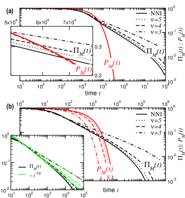
Figure 1: (Color online) $\nu$-dependence of the quantum mechanical $\Pi_{M}(t)$ and the classical $P_{M}(t)$ decay behaviors for a chain of $N=100$ sites; here (a) $\Gamma=0.001$ and (b) $\Gamma=1$. The inset in (a) shows a close-up picture of the region where $\Pi_{M}(t)$ and $P_{M}(t)$ cross. The inset in (b) shows power-law fits to $\Pi_{M}(t)$ in the intermediate time regime with exponents $1/\mu$, where the $\mu$ are taken from Fig. 3(b).

In Ref. Mülken et al. (2007) an experimental setup was proposed, which is based on a finite linear chain of clouds of ultracold Rydberg atoms with trapping states at both ends ($m=1,N$). There, the dynamics was approximated by a NNI tight binding model, which - for a ring without traps - has been shown to behave in the same fashion as systems with LRI of the form $R^{-\nu}$ for which $\nu>2$ Mülken et al. (2008). The Rydberg atoms interact via dipole-dipole forces, i.e., the potential between two atoms decays roughly as $R^{-3}$.

For the finite chain with $m=1,N$, Fig. 1 shows a comparison of the quantum mechanical $\Pi_{M}(t)$ and of the classical $P_{M}(t)$ behaviors for different $\nu$ and $\Gamma$, which were obtained by numerically diagonalizing the corresponding Hamiltonian ${\bf H}(\nu)$ and transfer matrix ${\bf T}(\nu)$, respectively. Clearly, for both $\Gamma$-values the LRI lead to a slower decay of $\Pi_{M}(t)$, i.e., to a slower trapping of the excitation, which is counter intuitive since the opposite effect is observable for classical systems where the decay of $P_{M}(t)$ becomes faster for decreasing $\nu$, see below. By increasing the trapping strength $\Gamma$, the difference between the quantum and the classical behavior becomes even more pronounced, compare Figs. 1(a) and 1(b). Generally, for $\Pi_{M}(t)$ the change in $\Gamma$ results mainly in a rescaled time axis, since the imaginary parts $\gamma_{l}$ are of the same order of magnitude when rescaled by $\Gamma$. For the specific case of the Rydberg atoms ($\nu=3$ and $\Gamma=1$) one observes the largest difference between the $\Pi_{M}(t)$ and the $P_{M}(t)$ behaviors. To understand this phenomenon, we continue to analyze $\Pi_{M}(t)$ within a perturbation theoretical treatment.

When the strength of the trap, $\Gamma$, is small compared to the couplings between neighboring nodes, we can evaluate the eigenvalues using perturbation theory, see, for instance, Sakurai (1994). Let $|\Psi^{(0)}_{l}\rangle$ be the $l$th eigenstate and $E^{(0)}_{l}\in\mathbb{R}$ be the $l$th eigenvalue of the unperturbed system with Hamiltonian ${\bf H}_{0}(\nu)$. Up to first-order the eigenvalues of the perturbed system are given by

$$E_{l}=E^{(0)}_{l}-i\Gamma\sum_{m\in{\cal M}}\Big{|}\langle m|\Psi^{(0)}_{l}\rangle\Big{|}^{2}.$$ (5)

Therefore, the correction term determines the imaginary parts $\gamma_{l}$, while the unperturbed eigenvalues are the real parts $\epsilon_{l}=E^{(0)}_{l}$. Having only a few trap nodes, the sum in Eq. (5) contains only few terms. Moreover, from Eq. (5) we also see that the imaginary parts $\gamma_{l}$ are essentially determined by the eigenstates $|\Psi^{(0)}_{l}\rangle$ of the system without traps. A change in these states will also lead to a change in the $\gamma_{l}$. As we proceed to show, this is exactly what happens by going from NNI to LRI.

Without loss of generality, an eigenstate of a finite chain with NNI can be written as ($l=1,\dots,N$)

$$|\Psi^{(0)}_{l}\rangle=\begin{cases}\displaystyle\sqrt{\frac{1}{N}}\sum_{j=1}^{N}|j\rangle&l=N\\ \displaystyle\sqrt{\frac{2}{N}}\sum_{j=1}^{N}\cos\big{[}(2j-1)\theta_{l}/2\big{]}|j\rangle&\mbox{else},\end{cases}$$ (6)

where for convenience we take $\theta_{l}\equiv\pi(N-l)/N\in[0,\pi[$; the corresponding eigenvalues are $E^{(0)}_{l}=2-2\cos\theta_{l}$ (note that the smallest eigenvalue is $E^{(0)}_{N}=0$). Thus, to first order perturbation theory we obtain from Eqs. (5) and (6) as imaginary parts $\gamma_{N}=2\Gamma/N$ and $\gamma_{l}=(4\Gamma/N)\cos^{2}\big{(}\theta_{l}/2\big{)}=(2\Gamma/N)[1+\cos\theta_{l}]$ for $l=1,\dots,N-1$, which for $l\ll N$ yields $\gamma_{l}\sim l^{2}$. In this case the mean survival probability will scale in the corresponding time interval as $\Pi_{M}(t)\sim t^{-1/2}$.

Formally, we can perform the continuum limit $N\to\infty$ (by taking now $4\Gamma/N\equiv a$ finite). Then the sum in Eq. (4) turns into an integral such that

$$\Pi_{M}(t)\sim e^{-at}\ \frac{1}{\pi}\int\limits_{0}^{\pi}d\theta\ e^{-at\cos\theta}=e^{-at}I_{0}(at),$$ (7)

where $I_{0}(at)$ is the modified Bessel function of the first kind Abramowitz and Stegun (1972). From this we get for large $t$ that $\Pi_{M}(t)\sim t^{-1/2}$, which confirms the previous results. Note, however, that for small $N$ the smallest $\gamma_{l}$-value is finite and, therefore, the scaling of $\gamma_{l}$ holds only in a quite small interval of $l$-values. Hence, also the time interval in which $\Pi_{M}(t)$ scales with the exponent $-1/2$ is rather small. A lower bound for scaling is given by the behavior of $\gamma_{l}$ for $l\approx N/2$ (corresponding to smaller times than for $l\ll N$). Here, $\gamma_{l}$ is linear in $l$, which leads to a lower bound of $\mu\geq 1$ for the scaling exponent. An exponent $\mu$ which is valid over a larger $l$-interval will therefore be in the interval $[1,2]$ and, consequently, the exponent for $\Pi_{M}(t)$ will lie in the interval $[-1,-1/2]$.

In the case of periodic boundary conditions, one finds translation-invariant Bloch eigenstates regardless of the range of the interaction Mülken et al. (2008). In the case of Eq. (1), however, the eigenstates for LRI differ from the ones for NNI [Eq. (6)]; In Eq. (1) the finite extension of the chain destroys the translational invariance. As is immediately clear from Eq. (5), this also implies that the imaginary parts of the eigenvalues, evaluated based on first order perturbation theory, will change.

For large exponents $\nu$ we can regard the LRI as a small perturbation to the NNI, i.e., having ${\bf H}_{0}(\nu)={\bf H}_{0}+{\bf H}_{\nu}$, where ${\bf H}_{\nu}$ contains only the correction terms to the NNI case ${\bf H}_{0}$. This allows us to calculate from the unperturbed states $|\Psi^{(0)}_{l}\rangle$ the perturbed eigenstates $|\Psi_{l}\rangle$ up to first order. Taking the states $|\Psi_{l}\rangle$ to be the eigenstates of the LRI system without traps, we readily obtain the imaginary parts $\gamma_{l}$ for small trapping strength from Eq. (5) as $\gamma_{l}=2\Gamma\big{|}\langle 1|\Psi_{l}\rangle\big{|}^{2}$, where

$$\langle 1|\Psi_{l}\rangle=\langle 1|\Psi^{(0)}_{l}\rangle+\sum_{r\neq l}\frac{\langle\Psi^{(0)}_{r}|{\bf H}_{\nu}|\Psi^{(0)}_{l}\rangle}{E^{(0)}_{l}-E^{(0)}_{r}}\langle 1|\Psi^{(0)}_{r}\rangle.$$ (8)

It is straightforward, although cumbersome, to calculate the corrections to the imaginary parts $\gamma_{l}$ from Eq. (8). For large $\nu$ the coupling to the next-next-nearest neighbor is by a factor of $(3/2)^{\nu}$ smaller, for $\nu=10$ this is about one and a half orders of magnitude. Taking, for fixed $\nu$, only nearest and next-nearest neighbor couplings into account allows us to obtain simple analytic expressions. The perturbation term ${\bf H}_{\nu}$ is now tri-diagonal. Its non-zero elements are $\langle j-2|{\bf H}_{\nu}|j\rangle=\langle j+2|{\bf H}_{\nu}|j\rangle=-2^{-\nu}$ and its diagonal elements follow from $\langle j|{\bf H}_{\nu}|j\rangle=-\sum_{i}\langle i|{\bf H}_{\nu}|j\rangle$, thus $\langle j|{\bf H}_{\nu}|j\rangle=2^{-\nu}$ for $2<j<N-1$ and $\langle j|{\bf H}_{\nu}|j\rangle=2^{-\nu+1}$ else. We hence obtain from Eq. (8)

$$\langle 1|\Psi_{l}\rangle=\sqrt{\frac{2}{N}}\cos\Big{(}\frac{\theta_{l}}{2}\Big{)}+2^{-\nu}\sqrt{\frac{2}{N}}\sin\big{(}2\theta_{l}\big{)}\sin\Big{(}\frac{\theta_{l}}{2}\Big{)}.$$ (9)

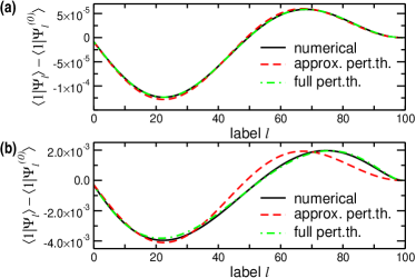
Figure 2: (Color online) Correction term $\langle 1|\Psi_{l}\rangle-\langle 1|\Psi^{(0)}_{l}\rangle$ for $N=100$ and for (a) $\nu=10$ and (b) $\nu=5$. The direct numerical evaluation (solid black line) is compared to the perturbation theory expression Eq. (8) (dashed-dotted green line) and to the approximate expression Eq. (9) (dashed red line).

Figure 2 shows the difference $\langle 1|\Psi_{l}\rangle-\langle 1|\Psi^{(0)}_{l}\rangle$ for $N=100$ and for (a) $\nu=10$ and (b) $\nu=5$. The numerical exact value (solid black line) is obtained by computing separately $\langle 1|\Psi_{l}\rangle$ and $\langle 1|\Psi^{(0)}_{l}\rangle$ and subsequently taking the difference; the result is then confronted to Eq. (8) (dashed-dotted green line), determined numerically, and to Eq. (9) (dashed red line). For $\nu=10$, the agreement between all three curves is remarkably good, see Fig. 2(a), which justifies the assumptions leading to Eq. (9). For smaller $\nu$ [$\nu=5$ in Fig. 2(b)] there is still a reasonable agreement between Eq. (8) and the exact result; however, taking only nearest and next-nearest neighbors into account leads to evident deviations, see the dashed red line in Fig. 2(b).

Now, from Eq. (9) we get

$$\gamma_{l}\approx\gamma_{l}^{(0)}+2^{-\nu}\gamma_{l}^{(1)}+{\cal O}(2^{-2\nu}),$$ (10)

where $\gamma_{l}^{(0)}$ is the NNI expression given above and $\gamma_{l}^{(1)}=(8\Gamma/N)\cos\big{(}\theta_{l}/2\big{)}\sin\big{(}2\theta_{l}\big{)}\sin\big{(}\theta_{l}/2\big{)}$ the correction due to the LRI. Again, the smallest $\gamma_{l}$-values are those for which $l\ll N$, which leads to a decrease of the imaginary parts $\gamma_{l}$ because $\gamma_{l}^{(1)}<0$ for $l\ll N$. Here, one can approximate the imaginary parts by a power-law, i.e., $\gamma_{l}\sim l^{\mu}$. A rough estimate of the scaling exponent $\mu$, assuming $\nu\gg 1$ can be readily given. For this we note that from Eq. (10) we have $\ln\gamma_{l+1}-\ln\gamma_{l}\approx\ln\gamma_{l+1}^{(0)}-\ln\gamma_{l}^{(0)}+2^{-\nu}\big{[}(\gamma_{l+1}^{(1)}/\gamma_{l+1}^{(0)}-\gamma_{l}^{(1)}/\gamma_{l}^{(0)}\big{]}$. Moreover, the term $\mu^{(0)}\equiv\big{[}\ln\gamma_{l+1}^{(0)}-\ln\gamma_{l}^{(0)}\big{]}/\big{[}\ln(l+1)-\ln l\big{]}$ gives the exponent for the NNI case and the term $\mu^{(1)}\equiv\big{[}\gamma_{l+1}^{(1)}/\gamma_{l+1}^{(0)}-\gamma_{l}^{(1)}/\gamma_{l}^{(0)}\big{]}/\big{[}\ln(l+1)-\ln l\big{]}$ is the LRI correction. Thus

$$\mu\approx\frac{\ln\gamma_{l+1}-\ln\gamma_{l}}{\ln(l+1)-\ln l}\approx\mu^{(0)}+2^{-\nu}\mu^{(1)}$$ (11)

Since $\mu^{(1)}$ is strictly positive for small $l$, the inclusion of LRI leads to a decrease of $\gamma_{l}$ when compared to the NNI case. In turn, this results in a slower decay of $\Pi_{M}(t)$.

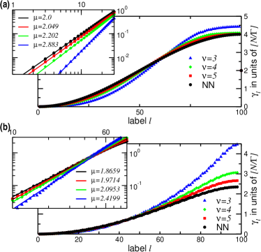
Figure 3: (Color online) Imaginary parts $\gamma_{l}$ (dots) in ascending order for LRI systems with $\nu=2$, $3$, $4$, and for NNI for $N=100$ and (a) $\Gamma=0.001$ and (b) $\Gamma=1$.

Figure 3 shows the imaginary parts $\gamma_{l}$ for a chain of $N=100$ nodes with LRI ($\nu=3$, $4$, $5$) and with NNI. For small $l$ and NNI, the $\gamma_{l}$ obey scaling with the exponent $\mu=2$, as discussed above. Introducting LRI, i.e., decreasing $\nu$, increases the scaling exponent to $\mu>2$. Consequently, the scaling exponent $1/\mu$ for $\Pi_{M}(t)$ decreases, leading to a slowing-down of the excitation trapping due to LRI.

In the classical case decreasing $\nu$ leads to a faster excitation trapping, which is obervable in a quicker decay of $P_{M}(t)$. This can also be deduced from a perturbation theoretical treatment. As can be seen from Fig. 1 (see also Fig. 2 of Ref. Mülken et al. (2007)), the decay of $P_{M}(t)$ is exponential already at intermediate times and is dominated by the smallest eigenvalue $\lambda_{N}$ and the corresponding eigenstate $|\Phi_{N}\rangle$ of the transfer operator ${\bf T}(\nu)$:

$$P_{M}(t) = \frac{1}{N-M}\sum_{l=1}^{N}\exp(-\lambda_{l}t)\Big{|}\sum_{k\not\in{\cal M}}\langle k|\Phi_{l}\rangle\Big{|}^{2}$$ (12)

$$\approx \frac{1}{N-M}\exp(-\lambda_{N}t)\Big{|}\sum_{k\not\in{\cal M}}\langle k|\Phi_{N}\rangle\Big{|}^{2}.$$

Calculating $\lambda_{N}$ and the prefactor $\big{|}\sum_{k\not\in{\cal M}}\langle k|\Phi_{N}\rangle\big{|}^{2}$ for large $\nu$ and small $\Gamma$ shows that with decreasing $\nu$ the smallest eigenvalue $\lambda_{N}$ increases while the prefactor decreases. Together, this confirms our numerical result of a quicker decay for $P_{M}(t)$, see Fig. 1.

Finally, we comment on the impact of our results on the experiment proposed in Ref. Mülken et al. (2007). Here, clouds of laser-cooled ground state atoms are assembled in a chain by optical dipole traps Grimm et al. (2000), which are then excited into a Rydberg S-state, see Mülken et al. (2007) for details. The Rydberg atoms interact via long-range dipole-dipole forces which is advantageous in many ways. As can be deduced from Fig. 1, the time intervals over which the decay follows the power-law are enlarged by the LRI. For $\nu=3$ the transition to the long-time exponential decay occurs at times which are about two order of magnitude larger than the ones found for the NNI case. The difference between a purely coherent (CTQW) and a purely incoherent (CTRW) process is enlarged due to the LRI, allowing for a better discrimination between the two when clarifying the nature of the energy transfer dynamics in ultra-cold Rydberg gases.

In conclusion, we have considered the quantum dynamics of excitations with LRI on a network in the presence of absorbing sites (traps). The LRI lead to a slowing-down of the decay of the average survival probability, which is counter intuitive since for the corresponding classical process one observes a speed-up of the decay. Using pertubation theory arguments we were able to identify the reason for this slowing-down; it results from changes in the imaginary parts of the spectrum of the Hamiltonian.

Support from the Deutsche Forschungsgemeinschaft (DFG) and the Fonds der Chemischen Industrie is gratefully acknowledged.

References

- Bloch (2005) I. Bloch, Nature Physics 1, 23 (2005); I. Bloch, J. Dalibard, and W. Zwerger, Rev. Mod. Phys., in press (2008).
- Farhi and Gutmann (1998) E. Farhi and S. Gutmann, Phys. Rev. A 58, 915 (1998).
- Mülken and Blumen (2005) O. Mülken and A. Blumen, Phys. Rev. E 71, 016101 (2005).
- Perets et al. (2007) H. B. Perets et al., Phys. Rev. Lett., in press (2008).
- Dür et al. (2002) W. Dür et al., Phys. Rev. A 66, 052319 (2002).
- Côté et al. (2006) R. Côté et al., New J. Phys. 8, 156 (2006).
- Mülken et al. (2007) O. Mülken et al., Phys. Rev. Lett. 99, 090601 (2007).
- Mülken et al. (2008) O. Mülken, V. Pernice, and A. Blumen, Phys. Rev. E 77, 021117 (2008).
- Lukin et al. (2001) M. D. Lukin et al., Phys. Rev. Lett. 87, 037901 (2001); K. Singer et al., Phys. Rev. Lett. 93, 163001 (2004).
- Ates et al. (2007a) C. Ates et al., Phys. Rev. Lett. 98, 023002 (2007a); Phys. Rev. A 76, 013413 (2007b).
- Klafter and Silbey (1980) J. Klafter and R. Silbey, J. Chem. Phys. 72, 849 (1980); P. Grassberger and I. Procaccia, J. Chem. Phys. 77, 6281 (1982).
- Pearlstein (1971) R. M. Pearlstein, J. Chem. Phys. 56, 2431 (1971); D. L. Huber, Phys. Rev. B 22, 1714 (1980); 45, 8947 (1992); P. E. Parris, Phys. Rev. Lett. 62, 1392 (1989a); Phys. Rev. B 40, 4928 (1989); V. A. Malyshev, R. Rodríguez, and F. Domínguez-Adame, J. Lumin. 81, 127 (1999).
- Sakurai (1994) J. Sakurai, Modern Quantum Mechanics (Addison-Wesley, Redwood City, CA, 1994), 2nd ed.
- Abramowitz and Stegun (1972) M. Abramowitz and I. A. Stegun, eds., Handbook of Mathematical Functions (Dover, New York, 1972).
- Grimm et al. (2000) R. Grimm, M. Weidemüller, and Y. B. Ovchinnikov, Adv. At. Mol. Opt. Phys. 42, 95 (2000).