$\pi B_{8}B_{8}$ and $\sigma B_{8}B_{8}$ couplings from a chiral quark potential model

Abstract

From an SU(2)$\otimes$SU(2) chiral quark potential model incorporating spontaneous chiral symmetry breaking the asymptotic $\pi$ and $\sigma$ exchange pieces of the $NN$ potential are generated. From them the $\pi NN$ and $\sigma NN$ coupling constants can be extracted. The generalization to SU(3)$\otimes$SU(3) allows for a determination of $\pi B_{8}B_{8}$ and $\sigma B_{8}B_{8}$ coupling constants according to exact SU(3) hadron symmetry. The implementation of the values of the couplings at $Q^{2}=0$ provided by QCD sum rules and/or phenomenology makes also feasible the extraction of the meson-baryon-baryon form factors. In this manner a quite complete knowledge of the couplings may be attained.

I Introduction

The meson-baryon-baryon $(mBB^{\prime})$ couplings play a central role in hadron physics concerning the baryon-baryon $(BB^{\prime})$ interactions as well as the formation and decay of baryon resonances. To study these couplings effective hadron lagrangians involving the mesons and baryons under consideration are postulated. All the complexity of the $mBB^{\prime}$ vertices is assumed to be taken into account through running couplings depending on $Q^{2}$, the transfer momentum in the vertex. This dependency is usually parametrized in terms of a form factor and a coupling constant defined as the value of the running coupling at a particular $Q^{2}$, usually on-shell $Q^{2}=M_{m}^{2}$. Then one can calculate physical processes and compare to data to extract these values. Thus the $\pi NN$ coupling constant is obtained from $\pi N$ and/or $NN$ scattering data Eri92 . For couplings involving baryons and/or mesons for which scattering or decay data are not so complete or unavailable one can also rely on symmetry to derive predictions, see for instance Sto96 .

From a more fundamental point of view hadrons are made up of quarks. Hence hadron structures and decays as well as hadron-hadron interactions should come out from quark dynamics as dictated by QCD. Due to the technical difficulty to achieve this objective at present quark models of hadrons incorporating QCD-motivated symmetries and dynamics have been successfully applied to generate the baryon-baryon interactions, and consistently the baryon spectrum, in the light $(u,d)$ Val05 as well as in the light + strange $(u,d,s)$ quark sectors Zha97 ; Shi00 ; Fuj07 . These models, sometimes less precise than effective hadronic treatments, offer the advantage of providing a consistent unified description of all baryon-baryon processes from the same hamiltonian at the quark level. This confers them in principle a great predictive power once the model parameters are tightly constrained from some selected set of existing data.

We shall make use of this power to predict, within a non-relativistic chiral quark model framework, $mB_{8}B_{8}$ ($B_{8}$: baryon of the flavor octet) coupling constants in terms of meson-quark-quark ($mqq)$ couplings. More precisely we shall generate, from a $mqq$ lagrangian incorporating the effect of spontaneous chiral symmetry breaking (SCSB), the quark-quark meson exchange potentials and from them, through a Born–Oppenheimer (BO) approximation, the asymptotic baryon–baryon meson exchange interactions. The use of justified harmonic oscillator baryon wave functions (in terms of quarks) will allow us to perform analytic calculations. By comparing the resulting interactions to the ones postulated at the effective hadronic level we shall identify the meson-baryon-baryon coupling constants. This procedure has been applied in the literature to the $\pi NN$ coupling Liu93 . Here we shall be more precise in the extraction of coupling constants and form factors and we shall extend its application to the $\sigma$ meson and the other $B_{8}$ baryons making feasible the comparison of our results to the ones obtained with alternative methods based on quark or hadron degrees of freedom.

The contents are organized as follows. In Sect. II we shall center on the light quark sector where spontaneously broken chiral SU(2)$\otimes$SU(2) symmetry serves as an underlying general guide to generate the quark-quark meson-exchange potentials. We shall revisit the calculation of the $\pi NN$ coupling in terms of the $\pi qq$ one and apply the same procedure to the $\sigma NN$ case. We shall also comment on the possibility of applying our method to $\Delta$ and nucleon resonances. Then in Sect. III we shall consider the extension, via chiral SU(3)$\otimes$SU(3), to the SU(3) octet of baryons. Finally in Sect. IV we shall summarize our main results and conclusions.

II Light quark sector: SU(2)$\mathbf{\otimes}$SU(2).

Our starting point is the chiral lagrangian

$$\mathcal{L}_{ch}=-g_{ch}\,\bar{q}\,(\openone_{SU(2)}\sigma\,+\,i\,\gamma_{5}\vec{\tau}\vec{\pi})q\,,$$ (1)

where $q$ has components $u$ and $d$, and $g_{ch}$ is the chiral $mqq$ coupling constant ($m:\pi,\sigma$). The spontaneous chiral symmetry breaking gives rise to a vertex form factor $F(Q^{2})$ Dia86 . From the parametrization given in references Fer86 ; Kus91 we propose the Lorentz invariant form (note that for the purpose of the derivation of static potentials $Q^{2}=-\vec{Q}^{2}$),

$$F(Q^{2})=\left(\frac{\Lambda^{2}}{\Lambda^{2}-Q^{2}}\right)^{1/2}\,,$$ (2)

where $\Lambda$ is an effective cutoff parameter fitted from data. We should keep in mind that this parametrization of $F(Q^{2})$ makes only sense for $Q^{2}<\Lambda^{2}.$

From the form proposed ($F(Q^{2}=0)=1)$ it is clear that $g_{ch}$ represents the value of the $mqq$ coupling, $g_{ch}F(Q^{2}),$ at $Q^{2}=M_{m}^{2}$ in the limit $M_{m}^{2}=0.$ In order to deal with coupling constants defined on the physical meson masses ($M_{\pi}^{2}\neq 0\neq M_{\sigma}^{2})$ we identify (it is implicitly assumed that $M_{\pi}^{2},M_{\sigma}^{2}<\Lambda^{2})$

$$g_{\pi qq}\equiv g_{ch}\left(\frac{\Lambda^{2}}{\Lambda^{2}-M_{\pi}^{2}}\right)^{1/2}$$ (3)

$$g_{\sigma qq}\equiv g_{ch}\left(\frac{\Lambda^{2}}{\Lambda^{2}-M_{\sigma}^{2}}\right)^{1/2}\,,$$ (4)

as the values of the coupling $g_{ch}F(Q^{2})$ at $Q^{2}=M_{\pi}^{2}$ and $Q^{2}=M_{\sigma}^{2}$, respectively.

Let us point out that the use of the experimental pion mass may have required the introduction of an explicit symmetry breaking term proportional to $\sigma$ in the lagrangian but this term has not any further effect in the analysis we perform. Regarding the $\sigma$ mass it will be taken as a parameter to be fitted from data around the value provided by the SCSB relation Sca82 ,

$$M_{\sigma}^{2}-M_{\pi}^{2}=4M_{q}^{2}\,$$ (5)

where $M_{q}$ denotes the constituent quark mass at $Q^{2}=0.$

In terms of $g_{\pi qq}$ we write the pion lagrangian as

$$\mathcal{L}_{\pi qq}=-g_{\pi qq}\text{ }\bar{q}\,\,i\gamma_{5}\vec{\tau}\vec{\pi}\,\,q\,$$ (6)

with a vertex form factor $F_{\pi qq}(Q^{2})$ given by

$$F_{\pi qq}(Q^{2})\equiv\left(\frac{\Lambda^{2}-M_{\pi}^{2}}{\Lambda^{2}-Q^{2}}\right)^{1/2}\,.$$ (7)

Analogously, the sigma lagrangian reads

$$\mathcal{L}_{\sigma qq}=-g_{\sigma qq}\bar{q}\,\,\openone_{SU(2)}\sigma\,\,q$$ (8)

with a vertex form factor $F_{\sigma qq}(Q^{2})$ given by

$$F_{\sigma qq}(Q^{2})\equiv\left(\frac{\Lambda^{2}-M_{\sigma}^{2}}{\Lambda^{2}-Q^{2}}\right)^{1/2}\,.$$ (9)

Note that both form factors are of the same type $F_{mqq}(Q^{2})\equiv\left(\Lambda^{2}-M_{m}^{2}/\Lambda^{2}-Q^{2}\right)^{1/2}$ so that $F_{mqq}(Q^{2}=M_{m}^{2})=1.$

II.1 $mqq$ and induced $mBB$ potentials

From $\mathcal{L}_{mqq}$ and the form factors the static OPE and OSE central potentials (to the respective lowest order in $Q^{2})$ can be obtained through a non-relativistic reduction of the corresponding Feynman diagram amplitudes. They are

$$V_{\mathrm{OPE}}^{ij}({\vec{r}}_{ij})={\frac{1}{3}}{\frac{g_{\pi qq}^{2}}{{4\pi}}}\,{\ \frac{M_{\pi}^{2}}{{4M_{i}M_{j}}}}\,\,M_{\pi}\,\left[\,Y(M_{\pi}\,r_{ij})-{\ \frac{\Lambda^{3}}{M_{\pi}^{3}}}\,Y(\Lambda\,r_{ij})\right]({\vec{\sigma}}_{i}\cdot{\vec{\sigma}}_{j})({\vec{\tau}}_{i}\cdot{\vec{\tau}}_{j})\,,$$ (10)

$$V_{\mathrm{OSE}}^{ij}({\vec{r}}_{ij})=-{\frac{g_{\sigma qq}^{2}}{{4\pi}}}\,\,M_{\sigma}\,\left[Y(M_{\sigma}\,r_{ij})-{\frac{\Lambda}{{M_{\sigma}}}}\,Y(\Lambda\,r_{ij})\right]\,.$$ (11)

Here $i$ and $j$ are numbers denoting quarks, $M_{i,j}=M_{q}$ , $\vec{\sigma}_{i,j}$ ($\vec{\tau}_{i,j})$ are the spin (isospin) Pauli operators, $r_{ij}$ is the interquark distance and the function $Y$ is defined as,

$$Y(x)\,=\,{\frac{e^{-x}}{x}}\,.$$ (12)

Once the potentials at the quark level have been derived we shall use them to obtain the baryon-baryon potentials. From $V_{\mathrm{OmE}}^{ij}$ the asymptotic baryon-baryon meson exchange static potential is defined as

$$(V_{q})_{\mathrm{OmE}}^{B_{a}B_{b}\rightarrow B_{c}B_{d}}(R\rightarrow\infty)\equiv\lim_{R\rightarrow\infty}<\Psi_{B_{c}B_{d}}|\sum_{\begin{subarray}{c}i\in B_{a},B_{c}\\ j\in B_{b},B_{d}\end{subarray}}V_{OmE}^{ij}|\Psi_{B_{a}B_{b}}>\,,$$ (13)

where $\Psi_{B_{i}B_{j}}$ stands for the two-baryon wave function, $R$ for the interbaryon distance and the integration is over the quark coordinates.

We shall concentrate on $B_{a}B_{b}\rightarrow B_{c}B_{d}$ interactions involving baryons with the same mass. Then the asymptotic two-baryon wave function will be expressed in the center of mass system as

$$\Psi_{B_{a}B_{b}}=\Phi_{B_{a}}(1,2,3;+\vec{R}/2)\,\,\Phi_{B_{b}}(4,5,6;-\vec{R}/2)$$ (14)

where $(1,2,3)$ and $(4,5,6)$ denote the quarks forming the baryons, $\pm\vec{R}/2$ the baryons position and

$$\Phi_{B_{i}}=(\Phi_{B_{i}})_{\mathrm{spatial}}(\Phi_{B_{i}})_{\mathrm{spin-flavor}}(\Phi_{B_{i}})_{\mathrm{color}}$$ (15)

is the one-baryon wave function expressed as the direct product of its spatial, spin–flavor and color parts. For the sake of simplicity the baryon spatial wave function will be chosen of harmonic oscillator type

$$(\Phi_{B})_{\mathrm{spatial}}(1,2,3;+{\vec{R}}/2)=\prod_{i=1}^{3}\left(\frac{1}{\pi b^{2}}\right)^{\frac{3}{4}}\exp\left[-\left(\vec{r}_{i}-\vec{R}/2\right)^{2}/2b^{2}\right]$$ (16)

with an harmonic oscillator parameter, $b$, related to the size of the baryon.

II.2 Parameters

In order to fix the parameters at the quark level: $M_{q}$, $M_{\pi}$, $M_{\sigma}$, $g_{ch}$, $\Lambda$, and $b$, we shall rely on the efficient description of $NN$ data provided by the Chiral Quark Cluster Model (CQCM) Val05 . Such model contains, apart from OPE and OSE potentials derived from $\mathcal{L}_{mqq}$, a confinement plus a residual one-gluon exchange (OGE) interactions. We should realize though that the precise fitting of the parameters in the CQCM relies on a RGM calculation so that the two-baryon wave function as well as the baryon-baryon potentials are different from the ones obtained via the Born-Oppenheimer (BO) approach we follow, Eq. (13). We shall take this into account in an effective manner by keeping the same values for $M_{q}$, $M_{\pi}$, $M_{\sigma}$, $\Lambda$, and $b$, and fitting a new value for $g_{ch}$ to reproduce, with our BO approach, the experimental value of the pion-nucleon-nucleon coupling constant (see next section). The values of the parameters used henceforth are listed in Table 1.

Table 1: Quark model parameters Val05 .

$M_{q}$	$b$	$M_{\sigma}$	$M_{\pi}$	$\Lambda$
(MeV)	(fm)	(fm-1)	(fm-1)	(fm-1)
313	0.518	3.42	0.7	4.2

II.3 $\mathbf{\pi NN}$

From Eqs. (10), (13) and (16) the asymptotic OPE central potential for $NN\rightarrow NN$, corresponding to the diagram of Fig. 1 (there are nine equivalent ones), can be obtained. It reads (the calculation has been explicitly done in Ref. Liu93 )

$$(V_{q})_{\mathrm{OPE}}^{NN\rightarrow NN}(R\rightarrow\infty)=\frac{g_{\pi qq}^{2}}{4\pi}\left[9<(\vec{\sigma}_{3}\cdot\vec{\sigma}_{6})_{NN}.(\vec{\tau}_{3}\cdot\vec{\tau}_{6})_{NN}>e^{\frac{M_{\pi}^{2}b^{2}}{2}}\right]\frac{M_{\pi}^{2}}{4M_{q}^{2}}\frac{1}{3}\frac{e^{-M_{\pi}R}}{R}\,.$$ (17)

Figure 1: Asymptotic $NN$ OPE or OSE interactions at quark level.

To extract the $\pi NN$ coupling we have to compare this potential with the one derived from a postulated hadronic lagrangian. Assuming for instance a pseudoscalar coupling we can write a lagrangian

$$\mathcal{L}_{\pi NN}=-(g_{\pi NN})_{Q^{2}=M_{\pi}^{2}}\,\bar{N}\,\,i\,\gamma_{5}\vec{\tau}\,\vec{\pi}\,\,N\,,$$ (18)

with a vertex form factor $G_{\pi NN}(Q^{2})$ so that $G_{\pi NN}(Q^{2}=M_{\pi}^{2})=1$. Notice that we have indicated explicitly the on-shell character of the coupling $g_{\pi NN}$ through the subindex. In order to derive from this lagrangian a Yukawa-like pion exchange potential, monopole or dipole type form factors are usually assumed. Concerning the asymptotic potential both give the same result. We shall use in parallel with the form factor at the quark level a form

$$G_{\pi NN}(Q^{2})\equiv\left(\frac{\Lambda_{\pi NN}^{2}-M_{\pi}^{2}}{\Lambda_{\pi NN}^{2}-Q^{2}}\right)^{\frac{1}{2}}\,,$$ (19)

valid for $Q^{2}<\Lambda_{\pi NN}^{2}$ and $M_{\pi}^{2}<\Lambda_{\pi NN}^{2}$ ($\Lambda_{\pi NN}$ is a cutoff parameter to be fitted).

Note that if we had preferred to refer the lagrangian to the value of the coupling at $Q^{2}=0,$ i.e., to $(g_{\pi NN})_{Q^{2}=0}$ , then we would have a different form factor such that

$$(g_{\pi NN})_{Q^{2}=M_{\pi}^{2}}\,\,G_{\pi NN}(Q^{2})=(g_{\pi NN})_{Q^{2}=0}\,\,\left(\frac{\Lambda_{\pi NN}^{2}}{\Lambda_{\pi NN}^{2}-Q^{2}}\right)^{\frac{1}{2}}\,,$$ (20)

where the second term on the right hand side represents the form factor normalized at $Q^{2}=0.$

From $\mathcal{L}_{\pi NN}$ and $G_{\pi NN}(Q^{2})$ the non-relativistic reduction of the one-pion exchange diagram, Fig. 2, to the lowest order in $Q^{2}$, provides us with the pion exchange static potential at the baryonic level. The asymptotic behavior of its central part is given by

$$(\mathcal{V}_{B})_{\mathrm{OPE}}^{NN\rightarrow NN}(R\rightarrow\infty)=\frac{(g_{\pi NN}^{2})_{Q^{2}=M_{\pi}^{2}}}{4\pi}\left[\left\langle(\vec{\sigma}_{N}\cdot\vec{\sigma}_{N})(\vec{\tau}_{N}\cdot\vec{\tau}_{N})\right\rangle\right]\frac{M_{\pi}^{2}}{4M_{N}^{2}}\,\,\frac{1}{3}\frac{e^{-M_{\pi}R}}{R}\,.$$ (21)

Figure 2: Asymptotic $NN$ OPE or OSE interactions at baryon level.

Note that $(\mathcal{V}_{B})_{\mathrm{OPE}}^{NN\rightarrow NN}(R\rightarrow\infty)$ only depends on the coupling constant and not on the form factor. Then no information on the form factors at the baryon level can be extracted from it. Regarding the coupling constant we can make use of the relation $(25/9)<(\vec{\sigma}_{N}\cdot\vec{\sigma}_{N})(\vec{\tau}_{N}\cdot\vec{\tau}_{N})>=9<(\vec{\sigma}_{3}\cdot\vec{\sigma}_{6})_{NN}.(\vec{\tau}_{3}\cdot\vec{\tau}_{6})_{NN}>$ Liu93 to compare Eqs. (17) and (21). From this comparison we extract

$$(g_{\pi NN}^{2})_{Q^{2}=M_{\pi}^{2}}=g_{\pi qq}^{2}\,\,\frac{M_{N}^{2}}{M_{q}^{2}}\,\,\frac{25}{9}\,\,e^{\frac{M_{\pi}^{2}b^{2}}{2}}\,.$$ (22)

Having chosen $M_{q}=313$ MeV so that $M_{N}=3M_{q}$ we can re-express

$$(g_{\pi NN}^{2})_{Q^{2}=M_{\pi}^{2}}=25\,\,g_{\pi qq}^{2}\,\,e^{\frac{M_{\pi}^{2}b^{2}}{2}}\,.$$ (23)

II.3.1 Pseudovector couplings

Alternatively to $g_{\pi qq}$ and $g_{\pi NN}$ we could have used pseudovector couplings $f_{\pi qq}$ and $f_{\pi NN}$ so that

$$\mathcal{L}_{\pi qq}^{PV}=-\frac{f_{\pi qq}}{M_{\pi}}\bar{q}\,\,i\gamma_{5}\gamma_{\mu}\vec{\tau}\partial^{\mu}\vec{\pi}\,\,q$$ (24)

with the vertex form factor $F_{\pi qq}(Q^{2})$ and

$$\mathcal{L}_{\pi NN}^{PV}=-\frac{(f_{\pi NN})_{Q^{2}=M_{\pi}^{2}}}{M_{\pi}}\,\bar{N}\,\,i\,\gamma_{5}\gamma_{\mu}\vec{\tau}\partial^{\mu}\vec{\pi}\,\,N\,.$$ (25)

with the vertex form factor $G_{\pi NN}(Q^{2}).$

It turns out that $\mathcal{L}^{PV}$ give rise to exactly the same potentials as $\mathcal{L}$ , to the lowest $Q^{2}$ order, under the identifications

$$\frac{f_{\pi qq}^{2}}{M_{\pi}^{2}}=\frac{g_{\pi qq}^{2}}{4M_{q}^{2}}$$ (26)

$$\frac{(f_{\pi NN}^{2})_{Q^{2}=M_{\pi}^{2}}}{M_{\pi}^{2}}=\frac{(g_{\pi NN}^{2})_{Q^{2}=M_{\pi}^{2}}}{4M_{N}^{2}}\,.$$ (27)

If we now substitute these relations in Eq. (22) we get

$$(f_{\pi NN}^{2})_{Q^{2}=M_{\pi}^{2}}=f_{\pi qq}^{2}\,\,\frac{25}{9}\,\,e^{\frac{M_{\pi}^{2}b^{2}}{2}}\,.$$ (28)

The corresponding constant $f_{ch}$ is consistently defined as

$$f_{ch}=\left(\frac{\Lambda^{2}-M_{\pi}^{2}}{\Lambda^{2}}\right)^{1/2}f_{\pi qq}=\lim_{M_{\pi}\rightarrow 0}f_{\pi qq}\,.$$ (29)

II.3.2 Coupling constants and form factor values

From a standard experimental value $(f_{\pi NN}^{2})_{Q^{2}=M_{\pi}^{2}}/4\pi\simeq 0.079$ (see Eri92 and references therein) or $(g_{\pi NN}^{2})_{Q^{2}=M_{\pi}^{2}}/4\pi\simeq 14.6$ we fit the pion-quark-quark coupling constant

$$f_{\pi qq}^{2}/4\pi=0.027$$ (30)

or

$$g_{\pi qq}^{2}/4\pi=0.55\,,$$ (31)

and

$$|g_{ch}|\equiv|f_{ch}|\,\dfrac{2\,M_{q}}{M_{\pi}}=2.6\,.$$ (32)

Let us emphasize that this value for $g_{ch}$ differs less than a 10% from the one obtained via QCD sum rules (QCDSR) $(g_{ch})_{\mathrm{QCDSR}}\simeq 2.83$ Hwa96 .

Regarding $\Lambda_{\pi NN}$, the cutoff parameter, its range of values can be estimated. In Ref. Hen91 a fit to data was attained from a gaussian form factor $e^{Q^{2}/\Lambda_{\mathrm{HM}}^{2}}$ with $\Lambda_{\mathrm{HM}}$ varying from $2.6$ to $4.2$ fm${}^{-1}.$ This form factor is normalized at $Q^{2}=0$. By requiring its low $Q^{2}$ behavior $(1+Q^{2}/\Lambda_{\mathrm{HM}}^{2}),$ to be the same than that of our form factor normalized at $Q^{2}=0$ in Eq. (20), $(1+Q^{2}/2\Lambda_{\pi NN}^{2})$, we get $\Lambda_{\mathrm{HM}}^{2}=2\Lambda_{\pi NN}^{2}$. Hence the resulting range for $\Lambda_{\pi NN}$ is

$$\Lambda_{\pi NN}=1.84-2.97\,\,\,\mathrm{fm}^{-1}\,.$$ (33)

From Eqs. (19) and (20) this range can be translated in an interval of values for the coupling at $Q^{2}=0$ :

$$\frac{(f_{\pi NN}^{2})_{Q^{2}=0}}{4\pi} = 0.068-0.075\,,$$

$$\frac{(g_{\pi NN}^{2})_{Q^{2}=0}}{4\pi} = 12.5-13.8\,.$$ (34)

These values are in perfect agreement with the phenomenological analysis done in Ref. Tho89 (let us comment that for the form factor used in this reference the range of values for the cutoff parameter is the same as for $\Lambda_{\mathrm{HM}}$). The preferred value in Ref. Tho89 is $(f_{\pi NN}^{2})_{Q^{2}=0}/4\pi\simeq 0.073$ which corresponds to $(g_{\pi NN}^{2})_{Q^{2}=0}/4\pi\simeq 13.5$. It is worthwhile to point out that this corresponds quite approximately to the $M_{\pi}\rightarrow 0$ limit of our expression $(f_{\pi NN}^{2})_{Q^{2}=M_{\pi}^{2}}=f_{\pi qq}^{2}\,(25/9)\,e^{\frac{M_{\pi}^{2}b^{2}}{2}}$, i.e.,

$$\dfrac{(f_{\pi NN}^{2})_{Q^{2}=M_{\pi}^{2}\rightarrow 0}}{4\pi}=\dfrac{f_{ch}^{2}}{4\pi}\frac{25}{9}=0.072$$ (35)

indicating the quite approximate Goldstone boson character of the pion.

II.4 $\mathbf{\sigma NN}$

By proceeding in exactly the same way for the $\sigma$ exchange we obtain from Eqs. (11), (13) and (16) at the quark level

$$(V_{q})_{\mathrm{OSE}}^{NN\rightarrow NN}(R\rightarrow\infty)=-\frac{g_{\sigma qq}^{2}}{4\pi}\,\,9\,\,e^{\frac{M_{\sigma}^{2}b^{2}}{2}}\,\,\frac{e^{-M_{\sigma}R}}{R}\,.$$ (36)

On the other hand from the hadronic lagrangian

$$\mathcal{L}_{\sigma NN}=-(g_{\sigma NN})_{Q^{2}=M_{\sigma}^{2}}\bar{N}\,\,\openone_{SU(2)}\sigma\,\,N\,,$$ (37)

with a vertex form factor

$$G_{\sigma NN}(Q^{2})=\left(\frac{\Lambda_{\sigma NN}^{2}-M_{\sigma}^{2}}{\Lambda_{\sigma NN}^{2}-Q^{2}}\right)^{\frac{1}{2}}\,,$$ (38)

we get

$$(\mathcal{V}_{B})_{\mathrm{OSE}}^{NN\rightarrow NN}(R\rightarrow\infty)=-\frac{(g_{\sigma NN}^{2})_{Q^{2}=M_{\sigma}^{2}}}{4\pi}\,\,\frac{e^{-M_{\sigma}R}}{R}\,.$$ (39)

From their comparison

$$(g_{\sigma NN}^{2})_{Q^{2}=M_{\sigma}^{2}}=9\,\,g_{\sigma qq}^{2}\,\,e^{\frac{M_{\sigma}^{2}b^{2}}{2}}\,.$$ (40)

Let us note that once the value of $g_{\pi qq}$ has been fitted our model predicts the value of $g_{\sigma qq}$ through

$$\frac{g_{\sigma qq}^{2}}{g_{\pi qq}^{2}}=\frac{\Lambda^{2}-M_{\pi}^{2}}{\Lambda^{2}-M_{\sigma}^{2}}\,.$$ (41)

Equivalently

$$\frac{(g_{\sigma NN}^{2})_{Q^{2}=M_{\sigma}^{2}}}{(g_{\pi NN}^{2})_{Q^{2}=M_{\pi}^{2}}}=\frac{9}{25}\,\,\frac{\Lambda^{2}-M_{\pi}^{2}}{\Lambda^{2}-M_{\sigma}^{2}}\,\,e^{\frac{(M_{\sigma}^{2}-M_{\pi}^{2})b^{2}}{2}}\,.$$ (42)

II.4.1 Coupling constant and form factor values

From Eq. (42) we predict

$$\frac{(g_{\sigma NN}^{2})_{Q^{2}=M_{\sigma}^{2}}}{4\pi}=68.2\,$$ (43)

and from Eq. (40)

$$\frac{g_{\sigma qq}^{2}}{4\pi}=1.59\,.$$ (44)

As mentioned above our asymptotic comparison does not give any information on the cutoff parameter $\Lambda_{\sigma NN}$. Nonetheless we can combine our result for the coupling constant with the value of the coupling at $Q^{2}=0$ provided by QCDSR to get an insight into it. From Ref. Erk06

$$\dfrac{(g_{\sigma NN})_{Q^{2}=0}}{g_{q}^{\sigma}}=3.9\pm 1.0.$$ (45)

If we tentatively identify $g_{q}^{\sigma}$ with our $g_{\sigma qq}$ ($=4.47)$ we get

$$\dfrac{\left(g_{\sigma NN}^{2}\right)_{Q^{2}=0}}{4\pi}=17.4\pm 4.5\,,$$ (46)

and using the relation $\left(g_{\sigma NN}^{2}\right)_{Q^{2}=0}=\left(g_{\sigma NN}^{2}\right)_{Q^{2}=M_{\sigma}^{2}}\,G_{\sigma NN}^{2}(Q^{2}=0)$ we extract

$$\Lambda_{\sigma NN}=\left(\frac{M_{\sigma}^{2}}{1-\frac{(g_{\sigma NN}^{2})_{Q^{2}=0}}{(g_{\sigma NN}^{2})_{Q^{2}=M_{\sigma}^{2}}}}\right)^{\frac{1}{2}}=3.97\pm 0.18\,\,\mathrm{fm}^{-1}\,.$$ (47)

It is again interesting to consider the limit $M_{\sigma}\rightarrow 0$ of Eq. (40)

$$\dfrac{(g_{\sigma NN}^{2})_{Q^{2}=M_{\sigma}^{2}\rightarrow 0}}{4\pi}=\dfrac{9g_{ch}^{2}}{4\pi}=4.8\,,$$ (48)

or

$$\dfrac{(g_{\sigma NN}^{2})_{Q^{2}=M_{\sigma}^{2}\rightarrow 0}}{g_{\mathrm{ch}}^{2}}=9$$ (49)

and compare it to the interval of values of the coupling at $Q^{2}=0$ from Eq. (46). As can be seen the $M_{\sigma}\rightarrow 0$ value from Eq. (48) is out of this interval. This might be interpreted as reflecting the non-Goldstone boson nature of the $\sigma.$

II.5 $\mathbf{\pi N\Delta}$

Strictly speaking our procedure to extract the couplings only makes sense when the lowest order expansion in $Q^{2}$ we follow is simultaneously valid at the baryonic level ($E_{B}\simeq M_{B})$ and at the quark level ($E_{q}\simeq M_{q})$. We do not expect this to be true for light-quark baryons in general since the quarks can move relativistically inside them. However the structure of the ground states, the $N$ (and $\Lambda,\Sigma,$ and $\Xi$ when considering $SU(3)),$ is well described by non-relativistic constituent quark models through the effective parameters in the quark-quark potential. Then we expect our procedure to make sense for them. Regarding other baryon states like $\Delta$ and $N(1440)$ one should be more cautious as we illustrate next.

In order to extract the $\pi N\Delta$ coupling constant we consider the $NN\rightarrow N\Delta$ interaction. According to the harmonic oscillator model we are using the spatial wave function of $\Delta$ has exactly the same structure than the $N$ one. However the real $\Delta$ differs from the $N.$ To implement the bigger size for $\Delta$ predicted by non-relativistic spectroscopic models we shall consider the possibility of a slightly different value for the size parameter. Thus the $\Delta$ spatial wave function we shall use is

$$(\Phi_{\Delta})_{\mathrm{spatial}}(4,5,6;+\vec{R}/2)=\prod_{i=4}^{6}\left(\frac{1}{\pi b_{\Delta}^{2}}\right)^{\frac{3}{4}}\exp\left[-{\left(\vec{r}_{i}-\vec{R}/2\right)^{2}/2b_{\Delta}^{2}}\right]$$ (50)

with a baryon size parameter, $b_{\Delta}$. One should also keep in mind that the mass of the $\Delta$ is a $30\%$ bigger than the mass of the $N$. In our harmonic oscillator quark model this means that the quarks in the $\Delta$ have more potential and kinetic energy (virial theorem) than the quarks in the $N$. According to our comments above this could give rise to corrections in the expression of the static potential at the quark level. Moreover due to the $\Delta-N$ mass difference the positions of the baryons in the initial and final states should not be the same. Therefore we should not expect an accurate prediction for the coupling constant in this case.

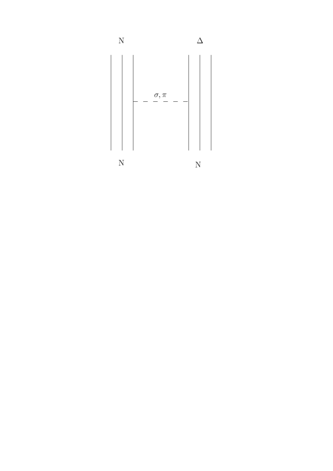
Figure 3: Asymptotic $NN\rightarrow N\Delta$ OPE or OSE interactions at quark level.

To derive such prediction we first calculate at the quark level, from Eqs. (13), (16) and (50) (we use for easiness the pseudovector form of the coupling) the asymptotic $NN\rightarrow N\Delta$ pion exchange static central potential, Fig. 3. It is

$$(V_{q})_{\mathrm{OPE}}^{NN\rightarrow N\Delta}(R\rightarrow\infty)=\frac{f_{\pi qq}^{2}}{4\pi}\left[\frac{160}{9\sqrt{2}}\,\,2\sqrt{2}\,\,\frac{b_{\mu}^{6}b_{+}^{3}b_{e}^{3}}{(b^{15}b_{\Delta}^{9})^{\frac{1}{2}}}e^{\frac{M_{\pi}^{2}b_{e}^{2}}{2}}\right]\frac{1}{3}\frac{e^{-M_{\pi}R}}{R}\,,$$ (51)

where the factor $160/9\sqrt{2}$ corresponds to $\left\langle N\Delta\left|(\vec{\sigma}_{3}\cdot\vec{\sigma}_{6})(\vec{\tau}_{3}\cdot\vec{\tau}_{6})\right|NN\right\rangle$ for total spin and isospin equal to 1, multiplied by 9 the number of equivalent diagrams, and $b_{\mu},b_{+}$ and $b_{e}$ are defined as

$$\frac{1}{b_{\mu}^{2}} = \frac{1}{2b^{2}}+\frac{1}{2b_{\Delta}^{2}}$$

$$\frac{1}{b_{\pm}^{2}} = \pm\frac{1}{b^{2}}+\frac{1}{b_{\mu}^{2}}$$ (52)

$$\frac{1}{b_{e}^{2}} = \frac{1}{2b_{+}^{2}}-\frac{b_{+}^{2}}{2b_{-}^{4}}\,.$$

Note that when $b_{\Delta}=b$ we also have $b_{e}=b_{\mu}=\sqrt{2}b_{+}=b$ hence reproducing, except for the spin-isospin factor, the $NN$ result.

At the baryonic level we have the lagrangians $\mathcal{L}_{\pi NN}^{PV}$ as given by Eq. (25) and

$$\mathcal{L}_{\pi N\Delta}^{PV}=-\frac{(f_{\pi N\Delta})_{Q^{2}=M_{\pi}^{2}}}{M_{\pi}}\,\,\bar{N}\,\,\vec{T}\partial\vec{\pi}\,\,\Delta\,,$$ (53)

with a form factor $G_{\pi N\Delta}(Q^{2})$ which we shall choose as,

$$G_{\pi N\Delta}(Q^{2})\equiv\left(\frac{\Lambda_{\pi N\Delta}^{2}-M_{\pi}^{2}}{\Lambda_{\pi N\Delta}^{2}-Q^{2}}\right)^{\frac{1}{2}}\,,$$ (54)

In Eq. (53) $\Delta$ corresponds to a Rarita-Schwinger $3/2$ spinor field and $\vec{T}$ is the isospin nucleon-delta transition operator. The corresponding pion exchange static central potential behaves asymptotically as

$$(\mathcal{V}_{B})_{\mathrm{OPE}}^{NN\rightarrow N\Delta}(R\rightarrow\infty)=\frac{(f_{\pi NN})_{Q^{2}=M_{\pi}^{2}}(f_{\pi N\Delta})_{Q^{2}=M_{\pi}^{2}}}{4\pi}\left[\left\langle(\vec{\sigma}_{N}\cdot\vec{S})(\vec{\tau}_{N}\cdot\vec{T})\right\rangle\right]\frac{1}{3}\,\frac{e^{-M_{\pi}R}}{R}$$ (55)

where $\vec{S}$ is the spin nucleon-delta transition operator and $\left\langle(\vec{\sigma}_{N}\cdot\vec{S})(\vec{\tau}_{N}\cdot\vec{T})\right\rangle=8/3$ for total spin and isospin equal to 1. Thus we identify,

$$\frac{(f_{\pi NN})_{Q^{2}=M_{\pi}^{2}}(f_{\pi N\Delta})_{Q^{2}=M_{\pi}^{2}}}{4\pi}=\frac{f_{\pi qq}^{2}}{4\pi}\left[\frac{20}{3\sqrt{2}}\,\,2\sqrt{2}\,\,\frac{b_{\mu}^{6}b_{+}^{3}b_{e}^{3}}{(b^{15}b_{\Delta}^{9})^{\frac{1}{2}}}\,\,e^{\frac{M_{\pi}^{2}b_{e}^{2}}{2}}\right]\,.$$ (56)

By using Eq. (28) we get,

$$\frac{(f_{\pi N\Delta})_{Q^{2}=M_{\pi}^{2}}}{(f_{\pi NN})_{Q^{2}=M_{\pi}^{2}}}=\left[\frac{6\sqrt{2}}{5}\,\,2\sqrt{2}\,\,\frac{b_{\mu}^{6}b_{+}^{3}b_{e}^{3}}{(b^{15}b_{\Delta}^{9})^{\frac{1}{2}}}\,\,e^{\frac{M_{\pi}^{2}(b_{e}^{2}-b^{2})}{2}}\right]$$ (57)

so that for $b_{\Delta}=b$ one obtains the usual spin-isospin relation ($f_{\pi N\Delta})_{Q^{2}=M_{\pi}^{2}}/(f_{\pi NN})_{Q^{2}=M_{\pi}^{2}}=6\sqrt{2}/5$.

For $b_{\Delta}$ in the interval $\left[b,1.2b\right]$ we predict $(f_{\pi N\Delta}^{2})_{Q^{2}=M_{\pi}^{2}}/4\pi=\left[0.23,0.20\right]$ to be compared to $(f_{\pi N\Delta}^{2})_{Q^{2}=M_{\pi}^{2}}/4\pi\simeq 0.37,$ estimated from the $\Delta$ decay to $N\pi.$ This discrepancy seems to confirm our initial expectations. If instead $f_{\pi qq}$ we had written an effective ($f_{\pi qq})_{N\Delta}$ as a manner to take into account the $\Delta-N$ mass difference effect then the needed value to reproduce the experimental number would have been $(f_{\pi qq})_{N\Delta}/f_{\pi qq}=\left[1.28,1.37\right]$ for $b_{\Delta}\in\left[b,1.2b\right]$, i.e. $(f_{\pi qq})_{N\Delta}$ should be a $30\%$ bigger than $f_{\pi qq}$.

For nucleon resonances in general and in particular for $N^{\ast}(1440)$ we expect the calculation of the coupling constants to be much more uncertain. As a matter of fact the importance of relativistic corrections in the description of the structure and decay of $N^{\ast}(1440)$ in terms of quarks have been emphasized for a long time in the literature (see for instance Can96 ). Furthermore the nature of the $N^{\ast}(1440)$ may involve more than a simple $3q$ structure and the coupling of $q\overline{q}$ pairs to the meson structure can be relevant. Therefore the calculation of $\pi NN^{\ast}(1440)$ and $\sigma NN^{\ast}(1440)$ coupling constants carried out in a preceding paper within the same framework Bru02 should be considered too simplistic. A less approximative calculation for the pion case (involving also $\pi N\Delta$, $\pi N\Delta(1600)$ and $\pi NN(1535))$ has been carried out in reference Bru04 with Poincaré covariant constituent quark models with instant, point and front forms of relativistic kinematics; from the persistent deviation from data of the calculated results the authors suggest the presence of sizable $qqqq\overline{q}$ components in the baryon wave functions.

III Light and strange quark sector: SU(3)$\mathbf{\otimes}$ SU(3).

The generalization of the chiral lagrangian to SU(3)$\otimes$SU(3) is straightforward. It is expressed as

$$\tilde{\mathcal{L}}_{ch}=-\tilde{g}_{ch}\,\,\bar{q}\,\left(\sum_{a=0}^{8}\sigma_{a}\lambda_{a}+i\sum_{a=0}^{8}\gamma_{5}\pi_{a}\lambda_{a}\right)\,q\,,$$ (58)

where $q$ has components $u,d$ and $s$, $\sigma_{0}$ and $\pi_{0}$ stand for the scalar and pseudoscalar meson singlets whereas $\sigma_{i}$ and $\pi_{i}$ $(i=1...8)$ are the scalar and pseudoscalar meson octets.

In order to derive a potential involving the exchange of $\sigma,$ the SU(2) singlet, we shall assume the ideal mixing

$$\sigma_{0} = \sqrt{2/3}\,\sigma+\sqrt{1/3}\,(s\overline{s})$$

$$\sigma_{8} = \sqrt{1/3}\,\sigma-\sqrt{2/3}\,(s\overline{s})\,.$$ (59)

When substituting these expressions in Eq. (58) the piece containing the $\sigma$ and the $\vec{\pi}$ read,

$$\tilde{\mathcal{L}}_{ch(\pi,\sigma)}=-\tilde{g}_{ch}\,\,\bar{q}\,\left[\sigma\left(\sqrt{2/3}\,\lambda_{0}+\sqrt{1/3}\,\lambda_{8}\right)+i\gamma_{5}\vec{\tau}\vec{\pi}\right]\,q$$ (60)

where $\lambda_{0}\equiv\sqrt{2/3}\,\openone_{\mathrm{SU(3)}}$ and $\lambda_{8}\equiv\sqrt{3}\,Y$, being $Y$ the hypercharge. It is then clear that for $q=u,d$ ($Yu=1/3=Yd)$ one formally recovers the SU(2)$\otimes$SU(2) lagrangian: $\openone_{\mathrm{SU(2)}}\equiv 2/3\,\openone_{\mathrm{SU(3)}}+Y$.

Again we take into account SCSB through a vertex form factor $\tilde{F}(Q^{2})$

$$\tilde{F}(Q^{2})=\left(\frac{\tilde{\Lambda}^{2}}{\tilde{\Lambda}^{2}-Q^{2}}\right)^{1/2}\,$$ (61)

Note also that the SCSB relation, $M_{\sigma}^{2}-M_{\pi}^{2}=4M_{q}^{2}$, is preserved since it is derived for a non-strange $\sigma$ Sca82 .

III.1 Parameters

One should realize that the values of the couplings $\tilde{g}_{ch}\,\tilde{F}(Q^{2})$ (or equivalently the on-shell couplings $\tilde{g}_{\pi qq}$, $\tilde{g}_{\sigma qq}$ and the cutoff parameter $\tilde{\Lambda}$) and the size parameter $\tilde{b}$ in SU(3)$\otimes$SU(3) need not be the same as in SU(2)$\otimes$SU(2). This is easily understandable by thinking for instance of the extra contribution to the $NN$ interaction coming from $\eta$, $\eta^{\prime}$ and $a_{0}$ in SU(3)$\otimes$SU(3). This contribution is taken into account in an effective manner in SU(2)$\otimes$SU(2), where no $\eta$, $\eta^{\prime}$, and $a_{0}$ are present, through the fitted values of $g_{\pi qq}$, $g_{\sigma qq}$, $\Lambda$ and $b$. Fortunately we can correlate the variations of $b$ and $\Lambda$ (or $\tilde{b}$ and $\tilde{\Lambda})$ through the relation Eq. (42),

$$\frac{(g_{\sigma NN}^{2})_{Q^{2}=M_{\sigma}^{2}}}{(g_{\pi NN}^{2})_{Q^{2}=M_{\pi}^{2}}}=\frac{9}{25}\,\,\frac{\Lambda^{2}-M_{\pi}^{2}}{\Lambda^{2}-M_{\sigma}^{2}}\,\,e^{\frac{(M_{\sigma}^{2}-M_{\pi}^{2})b^{2}}{2}}=\frac{9}{25}\,\,\frac{\tilde{\Lambda}^{2}-M_{\pi}^{2}}{\tilde{\Lambda}^{2}-M_{\sigma}^{2}}\,\,e^{\frac{(M_{\sigma}^{2}-M_{\pi}^{2})\tilde{b}^{2}}{2}}\,.$$ (62)

Then from the selected experimental value $(g_{\pi NN}^{2})_{Q^{2}=M_{\pi}^{2}}/4\pi\simeq 14.6$ and from our prediction $(g_{\sigma NN}^{2})_{Q^{2}=M_{\sigma}^{2}}/4\pi=68.2$ we get, for a typical value of $\tilde{\Lambda}\simeq 5.2$ fm^-1 ($\simeq$ 1.0 GeV) (note that it has to be higher than any mass of the scalar or pseudoscalar meson octets) an harmonic oscillator parameter $\tilde{b}\simeq 0.6$ fm. Then from equivalent relations to Eqs. (23) and (40) we get

$$\frac{\tilde{g}_{\pi qq}^{2}}{4\pi}=0.54$$ (63)

$$\frac{\tilde{g}_{\sigma qq}^{2}}{4\pi}=0.93\,,$$ (64)

and

$$\tilde{g}_{ch}=g_{ch}\,.$$ (65)

For the sake of completeness we give the $B_{8}$ spatial wave function in the SU(3)_flavor limit,

$$(\Phi_{B_{8}})_{\mathrm{spatial}}(1,2,3;+\vec{R}/2)=\prod_{i=1}^{3}\left(\frac{1}{\pi\tilde{b}^{2}}\right)^{\frac{3}{4}}\exp\left[-\left(\vec{r}_{i}-\vec{R}/2\right)^{2}/2\tilde{b}^{2}\right]\,.$$ (66)

III.2 $\mathbf{\sigma B_{8}B_{8}}$

According to our preceding discussions the $\sigma qq$ lagrangian will be written as

$$\tilde{\mathcal{L}}_{\sigma qq}=-\tilde{g}_{\sigma qq}\,\,\bar{q}\,\openone_{\mathrm{SU(2)}}\,\sigma\,\,q\,,$$ (67)

with a vertex form factor

$$\tilde{F}_{\sigma qq}(Q^{2})\equiv\left(\frac{\tilde{\Lambda}^{2}-M_{\sigma}^{2}}{\tilde{\Lambda}^{2}-Q^{2}}\right)^{1/2}\,.$$ (68)

Figure 4: Asymptotic $\Lambda\Lambda$, $\Sigma\Sigma$, and $\Xi\Xi$ OPE and OSE interactions at quark level. Thin lines stand for light ($u,d$) quarks and thick lines for strange ($s$) quarks.

From this lagrangian it is clear that the only difference when calculating the asymptotic potential at the quark level for the several $B_{8}B_{8}$’s has to do with the number of the pairs of light quarks ($u,d)$ in them allowing for the exchange of the $\sigma$, i.e., with the number of equivalent diagrams, Figs. 1 and 4. This number is 9 for $NN,$ 4 for $\Lambda\Lambda$ and $\Sigma\Sigma$, and 1 for $\Xi\Xi$. Thus

$$(\tilde{V}_{q})_{\mathrm{OSE}}^{\Lambda\Lambda\rightarrow\Lambda\Lambda}(R\rightarrow\infty) = (\tilde{V}_{q})_{\mathrm{OSE}}^{\Sigma\Sigma\rightarrow\Sigma\Sigma}(R\rightarrow\infty)=\frac{4}{9}(\tilde{V}_{q})_{\mathrm{OSE}}^{NN\rightarrow NN}(R\rightarrow\infty)$$

$$(\tilde{V}_{q})_{\mathrm{OSE}}^{\Xi\Xi\rightarrow\Xi\Xi}(R\rightarrow\infty) = \frac{1}{9}(\tilde{V}_{q})_{\mathrm{OSE}}^{NN\rightarrow NN}(R\rightarrow\infty)\,.$$ (69)

On the other hand at the baryonic level we shall write the lagrangian as

$$\mathcal{L}_{\sigma B_{8}B_{8}}\equiv-(g_{\sigma B_{8}B_{8}})_{Q^{2}=M_{\sigma}^{2}}\,\,\bar{B_{8}}\,\sigma\,\,B_{8}\,,$$ (70)

with a vertex form factor

$$G_{\sigma B_{8}B_{8}}(Q^{2})=\left(\frac{\Lambda_{\sigma B_{8}B_{8}}^{2}-M_{\sigma}^{2}}{{\Lambda_{\sigma B_{8}B_{8}}^{2}-Q^{2}}}\right)^{1/2}\,.$$ (71)

so that $G_{\sigma B_{8}B_{8}}(Q^{2}=M_{\sigma}^{2})=1$ and where the $(g_{\sigma B_{8}B_{8}})_{Q^{2}=M_{\sigma}^{2}}\,$ are expressed in conventional notation

$$(g_{\sigma NN})_{Q^{2}=M_{\sigma}^{2}}\, \equiv \sqrt{2/3}\,g_{s,1}+1/3\,g_{s,+}\,(4\alpha_{s}-1)$$

$$(g_{\sigma\Lambda\Lambda})_{Q^{2}=M_{\sigma}^{2}}\, \equiv \sqrt{2/3}\,g_{s,1}-2/3\,g_{s,+}\,(1-\alpha_{s})$$

$$(g_{\sigma\Sigma\Sigma})_{Q^{2}=M_{\sigma}^{2}}\, \equiv \sqrt{2/3}g_{s,1}+2/3\,g_{s,+}\,(1-\alpha_{s})$$ (72)

$$(g_{\sigma\Xi\Xi})_{Q^{2}=M_{\sigma}^{2}}\, \equiv \sqrt{2/3}\,g_{s,1}-1/3\,g_{s,+}\,(1+2\alpha_{s})\,,$$

being $g_{s,1}\equiv(g_{\sigma_{0}B_{8}B_{8}})_{Q^{2}=M_{\sigma}^{2}}$ the scalar SU(3) singlet coupling constant, $g_{s,+}\equiv g_{s,D}+g_{s,F}$ the sum of the $D$ (symmetric) and the $F$ (antisymmetric) scalar coupling constants in SU(3) and $\alpha_{s}\equiv g_{s,F}/g_{s,+}$ the $F/(F+D)$ ratio of the scalar octet.

From this baryonic lagrangian the following relations between the asymptotic potentials come out

$$(\mathcal{V}_{B})_{\mathrm{OSE}}^{\Lambda\Lambda\rightarrow\Lambda\Lambda}\,(R\rightarrow\infty) = \frac{(g_{\sigma\Lambda\Lambda}^{2})_{Q^{2}=M_{\sigma}^{2}}}{(g_{\sigma NN}^{2})_{Q^{2}=M_{\sigma}^{2}}}(\mathcal{V}_{B})_{\mathrm{OSE}}^{NN\rightarrow NN}\,(R\rightarrow\infty)$$

$$(\mathcal{V}_{B})_{\mathrm{OSE}}^{\Sigma\Sigma\rightarrow\Sigma\Sigma}\,(R\rightarrow\infty) = \frac{(g_{\sigma\Sigma\Sigma}^{2})_{Q^{2}=M_{\sigma}^{2}}}{(g_{\sigma NN}^{2})_{Q^{2}=M_{\sigma}^{2}}}(\mathcal{V}_{B})_{\mathrm{OSE}}^{NN\rightarrow NN}\,(R\rightarrow\infty)$$ (73)

$$(\mathcal{V}_{B})_{\mathrm{OSE}}^{\Xi\Xi\rightarrow\Xi\Xi}\,(R\rightarrow\infty) = \frac{(g_{\sigma\Xi\Xi}^{2})_{Q^{2}=M_{\sigma}^{2}}}{(g_{\sigma NN}^{2})_{Q^{2}=M_{\sigma}^{2}}}(\mathcal{V}_{B})_{\mathrm{OSE}}^{NN\rightarrow NN}\,(R\rightarrow\infty)\,.$$

From the comparison of the asymptotic potentials at the quark and baryon levels we immediately get relations between the coupling constants

$$\frac{(g_{\sigma\Lambda\Lambda}^{2})_{Q^{2}=M_{\sigma}^{2}}}{(g_{\sigma NN}^{2})_{Q^{2}=M_{\sigma}^{2}}} = \frac{(g_{\sigma\Sigma\Sigma}^{2})_{Q^{2}=M_{\sigma}^{2}}}{(g_{\sigma NN}^{2})_{Q^{2}=M_{\sigma}^{2}}}=\frac{4}{9}$$

$$\frac{(g_{\sigma\Xi\Xi}^{2})_{Q^{2}=M_{\sigma}^{2}}}{(g_{\sigma NN}^{2})_{Q^{2}=M_{\sigma}^{2}}} = \frac{1}{9}\,.$$ (74)

We should emphasize that these ratios are preserved in the limit $M_{\sigma}\rightarrow 0$, i.e.,

$$\frac{(g_{\sigma\Lambda\Lambda}^{2})_{Q^{2}=M_{\sigma}^{2}\rightarrow 0}}{(g_{\sigma NN}^{2})_{Q^{2}=M_{\sigma}^{2}\rightarrow 0}} = \frac{(g_{\sigma\Sigma\Sigma}^{2})_{Q^{2}=M_{\sigma}^{2}\rightarrow 0}}{(g_{\sigma NN}^{2})_{Q^{2}=M_{\sigma}^{2}\rightarrow 0}}=\frac{4}{9}$$

$$\frac{(g_{\sigma\Xi\Xi}^{2})_{Q^{2}=M_{\sigma}^{2}\rightarrow 0}}{(g_{\sigma NN}^{2})_{Q^{2}=M_{\sigma}^{2}\rightarrow 0}} = \frac{1}{9}\,.$$ (75)

It is interesting to compare these $M_{\sigma}\rightarrow 0$ ratios with the average QCDSR predictions at $Q^{2}=0$ in the SU(3) limit. From Ref. Oka06 we take

$$\frac{(g_{\sigma\Lambda\Lambda}^{2})_{Q^{2}=0}}{(g_{\sigma NN}^{2})_{Q^{2}=0}} = (0.43)^{2}=0.19$$

$$\frac{(g_{\sigma\Sigma\Sigma}^{2})_{Q^{2}=0}}{(g_{\sigma NN}^{2})_{Q^{2}=0}} = (0.91)^{2}=0.83$$

$$\frac{(g_{\sigma\Xi\Xi}^{2})_{Q^{2}=0}}{(g_{\sigma NN}^{2})_{Q^{2}=0}} = (0.08)^{2}=0.006.$$ (76)

As can be checked our ratios differ by a factor $2$ ($1/2)$ for $\Lambda-N$ and $\Sigma-N$ ($\Xi-N)$ from the QCDSR ones. We may interpret this again as a reflection of the non-Goldstone character of the $\sigma$ meson.

III.2.1 Coupling constants and form factors values

From Eq. (74) and from the calculated value $(g_{\sigma NN}^{2})_{Q^{2}=M_{\sigma}^{2}}/4\pi=68.2$ we predict the coupling constants

$$\frac{(g_{\sigma\Lambda\Lambda}^{2})_{Q^{2}=M_{\sigma}^{2}}}{4\pi} = \frac{(g_{\sigma\Sigma\Sigma}^{2})_{Q^{2}=M_{\sigma}^{2}}}{4\pi}=30.3$$

$$\frac{(g_{\sigma\Xi\Xi}^{2})_{Q^{2}=M_{\sigma}^{2}}}{4\pi} = 7.6\,.$$ (77)

Concerning the $F/(F+D)$ ratio we have from Eq. (74) $(g_{\sigma\Lambda\Lambda})_{Q^{2}=M_{\sigma}^{2}}=(g_{\sigma\Sigma\Sigma})_{Q^{2}=M_{\sigma}^{2}}$ what implies from Eq. (72)

$$\alpha_{s}=1\,,$$ (78)

or

$$g_{S,D}=0.$$ (79)

Regarding $g_{s,1}$ and $g_{S,+}$ we can use the fact that from the ideal mixing we have assumed $g_{(s\overline{s})NN}=-1/\sqrt{3}\,g_{s,1}+\sqrt{2}\,g_{s,F}-\sqrt{2}/3\,g_{s,D}=0$. Then from Eq. (79) we immediately obtain $g_{s,+}=1/\sqrt{6}\,g_{s,1}.$ If we substitute this relation and Eq. (78) in the first expression of Eq. (72) we get $(g_{\sigma NN})_{Q^{2}=M_{\sigma}^{2}}=3g_{s,+}$ from where

$$\frac{g_{s,+}^{2}}{4\pi} = 7.6$$ (80)

$$\frac{g_{s,1}^{2}}{4\pi} = 45.5\,,$$ (81)

satisfying

$$\dfrac{g_{s,1}^{2}}{g_{s,+}^{2}}=6\,.$$ (82)

With respect to the cutoff parameters $\Lambda_{\sigma B_{8}B_{8}}$ we can tentatively use our on-shell couplings ratios, Eq. (74), altogether with the QCDSR ones at $Q^{2}=0$ detailed above, Eq. (76), to establish a range of variation for them. Explicitly we can write

$$\left(\frac{(g_{\sigma B_{8}B_{8}}^{2})_{Q^{2}=0}}{(g_{\sigma NN}^{2})_{Q^{2}=0}}\right)=\left(\frac{(g_{\sigma B_{8}B_{8}}^{2})_{Q^{2}=M_{\sigma}^{2}}}{(g_{\sigma NN}^{2})_{Q^{2}=M_{\sigma}^{2}}}\right)\frac{\left(\frac{\Lambda_{\sigma B_{8}B_{8}}^{2}-M_{\sigma}^{2}}{{\Lambda_{\sigma B_{8}B_{8}}^{2}}}\right)}{\left(\frac{\Lambda_{\sigma NN}^{2}-M_{\sigma}^{2}}{\Lambda_{\sigma NN}^{2}}\right)}\,,$$ (83)

or equivalently

$$\Lambda_{\sigma B_{8}B_{8}}=\Lambda_{\sigma NN}\left(\frac{M_{\sigma}^{2}}{\Lambda_{\sigma NN}^{2}(1-x_{B_{8}})+x_{B_{8}}M_{\sigma}^{2}}\right)^{\frac{1}{2}}\,,$$ (84)

where

$$x_{B_{8}}\equiv\frac{\left(\frac{(g_{\sigma B_{8}B_{8}}^{2})_{Q^{2}=0}}{(g_{\sigma NN}^{2})_{Q^{2}=0}}\right)}{\left(\frac{(g_{\sigma B_{8}B_{8}}^{2})_{Q^{2}=M_{\sigma}^{2}}}{(g_{\sigma NN}^{2})_{Q^{2}=M_{\sigma}^{2}}}\right)}\,.$$ (85)

By using the average value $\Lambda_{\sigma NN}=3.97$ fm^-1, Eq. (47), we get

$$\Lambda_{\sigma NN} = 3.97\,\mathrm{{fm}^{-1}}$$

$$\Lambda_{\sigma\Lambda\Lambda} = 4.48\,\mathrm{{fm}^{-1}}$$

$$\Lambda_{\sigma\Sigma\Sigma} = 4.75\,\mathrm{{fm}^{-1}}$$ (86)

$$\Lambda_{\sigma\Xi\Xi} = 3.45\,\mathrm{{fm}^{-1}\,}\,.$$

Thus we can use $\Lambda_{\sigma B_{8}B_{8}}\simeq 4.0\,\mathrm{{fm}^{-1}}$ as an average value for the whole baryon octet.

III.3 $a_{0}\mathbf{B_{8}B_{8}}$

The results obtained for $\sigma$ can be extrapolated to the $a_{0}$ meson in a straightforward way. Let us recall that in the additive constituent quark pattern one has degenerate masses $M_{a_{0}}=M_{\sigma}$ (see Ref. Sca82 for an explanation of the non–degeneracy). Then by writing the $a_{0}$ on–shell couplings in SU(3) language

$$(g_{a_{0}NN})_{Q^{2}=M_{a_{0}}^{2}} = g_{s,+}$$

$$(g_{a_{0}\Sigma\Sigma})_{Q^{2}=M_{a_{0}}^{2}} = 2g_{s,+}\alpha_{s}$$ (87)

$$(g_{a_{0}\Xi\Xi})_{Q^{2}=M_{a_{0}}^{2}} = g_{s,+}(2\alpha_{s}-1)\,,$$

and imposing the degeneracy we predict from our value for $g_{s,+}$ (Eq. (80))

$$\dfrac{(g_{a_{0}NN}^{2})_{Q^{2}=M_{a_{0}}^{2}}}{4\pi} = \dfrac{(g_{a_{0}\Xi\Xi}^{2})_{Q^{2}=M_{a_{0}}^{2}}}{4\pi}=7.6$$

$$\dfrac{(g_{a_{0}\Sigma\Sigma}^{2})_{Q^{2}=M_{a_{0}}^{2}}}{4\pi} = 30.3\,.$$ (88)

III.4 $\mathbf{\pi B_{8}B_{8}}$

In order to avoid mass factors we shall use the pseudovector coupling for the pion, i.e., the lagrangian

$$\tilde{\mathcal{L}}_{\pi qq}^{PV}=-\frac{\tilde{f}_{\pi qq}}{M_{\pi}}\bar{q}\,\,i\gamma_{5}\gamma_{\mu}\vec{\tau}\partial^{\mu}\vec{\pi}\,\,q$$ (89)

with the vertex form factor

$$\tilde{F}_{\pi qq}(Q^{2})\equiv\left(\frac{\tilde{\Lambda}^{2}-M_{\pi}^{2}}{\tilde{\Lambda}^{2}-Q^{2}}\right)^{1/2}$$ (90)

to derive the asymptotic pion exchange central potentials. To perform the calculation we choose a total (spin, isospin) in each case. By considering the ${}^{1}S_{0}$ partial wave for instance we take $(0,1)$ for $NN$ and $\Xi\Xi$ and $(0,0)$ for $\Sigma\Sigma$ interactions. Then we have

$$(V_{q})_{\mathrm{OPE}}^{NN\rightarrow NN}\,(R\rightarrow\infty) = \frac{\tilde{f}_{\pi qq}^{2}}{4\pi}\left[-\frac{75}{9}\,e^{\frac{M_{\pi}^{2}\tilde{b}^{2}}{2}}\right]\frac{1}{3}\,\frac{e^{-M_{\pi}R}}{R}$$

$$(V_{q})_{\mathrm{OPE}}^{\Sigma\Sigma\rightarrow\Sigma\Sigma}\,(R\rightarrow\infty) = \frac{\tilde{f}_{\pi qq}^{2}}{4\pi}\left[\frac{32}{3}\,e^{\frac{M_{\pi}^{2}\tilde{b}^{2}}{2}}\right]\frac{1}{3}\,\frac{e^{-M_{\pi}R}}{R}$$ (91)

$$(V_{q})_{\mathrm{OPE}}^{\Xi\Xi\rightarrow\Xi\Xi}\,(R\rightarrow\infty) = \frac{\tilde{f}_{\pi qq}^{2}}{4\pi}\left[-\frac{3}{9}\,e^{\frac{M_{\pi}^{2}\tilde{b}^{2}}{2}}\right]\frac{1}{3}\,\frac{e^{-M_{\pi}R}}{R}\,.$$

On the other hand at the baryonic level the lagrangians can be expressed as

$$\mathcal{L}_{\pi NN}^{PV}=-\frac{(f_{\pi NN})_{Q^{2}=M_{\pi}^{2}}}{M_{\pi}}\,\bar{N}\,i\gamma_{5}\gamma_{\mu}\,\vec{\tau}\,\partial^{\mu}\vec{\pi}\,\,N$$ (92)

$$\mathcal{L}_{\pi\Sigma\Sigma}^{PV}=-\frac{(f_{\pi\Sigma\Sigma})_{Q^{2}=M_{\pi}^{2}}}{M_{\pi}}(\vec{\bar{\Sigma}}\times\vec{\Sigma}\,)\gamma_{5}\,\gamma_{\mu}\,\partial^{\mu}\vec{\pi}$$ (93)

$$\mathcal{L}_{\pi\Xi\Xi}^{PV}=-\frac{(f_{\pi\Xi\Xi})_{Q^{2}=M_{\pi}^{2}}}{M_{\pi}}\,\bar{\Xi}\,i\gamma_{5}\,\gamma_{\mu}\,\vec{\tau}\,\partial^{\mu}\,\vec{\pi}\,\Xi\,,$$ (94)

with form factors

$$G_{\pi NN}(Q^{2}) = \left(\frac{\Lambda_{\pi NN}^{2}-M_{\pi}^{2}}{\Lambda_{\pi NN}^{2}-Q^{2}}\right)^{\frac{1}{2}}$$

$$G_{\pi\Sigma\Sigma}(Q^{2}) = \left(\frac{\Lambda_{\pi\Sigma\Sigma}^{2}-M_{\pi}^{2}}{\Lambda_{\pi\Sigma\Sigma}^{2}-Q^{2}}\right)^{\frac{1}{2}}$$ (95)

$$G_{\pi\Xi\Xi}(Q^{2}) = \left(\frac{\Lambda_{\pi\Xi\Xi}^{2}-M_{\pi}^{2}}{\Lambda_{\pi\Xi\Xi}^{2}-Q^{2}}\right)^{\frac{1}{2}}\,,$$ (96)

and where in conventional SU(3) notation

$$(f_{\pi NN})_{Q^{2}=M_{\pi}^{2}} = f_{p,+}$$

$$(f_{\pi\Sigma\Sigma})_{Q^{2}=M_{\pi}^{2}} = 2f_{p,+}\,\alpha_{p}$$

$$(f_{\pi\Xi\Xi})_{Q^{2}=M_{\pi}^{2}} = -f_{p,+}(1-2\alpha_{p})\,,$$

having introduced $f_{p,+}\equiv(f_{p,D}+f_{p,F})$ as the sum of the symmetric and antisymmetric pseudoscalar octet coupling constants, and $\alpha_{p}\equiv f_{P,F}/(f_{P,D}+f_{P,F})$ as the $F/(F+D)$ ratio of the pseudoscalar octet.

By using the same total (spin, isospin) channels as above the corresponding asymptotic pion exchange central potentials are

$$(\mathcal{V}_{B})_{\mathrm{OPE}}^{NN\rightarrow NN}\,(R\rightarrow\infty) = \frac{(f_{\pi NN}^{2})_{Q^{2}=M_{\pi}^{2}}}{4\pi}\left[-3\right]\frac{1}{3}\frac{e^{-M_{\pi}R}}{R}$$

$$(\mathcal{V}_{B})_{\mathrm{OPE}}^{\Sigma\Sigma\rightarrow\Sigma\Sigma}\,(R\rightarrow\infty) = \frac{(f_{\pi\Sigma\Sigma}^{2})_{Q^{2}=M_{\pi}^{2}}}{4\pi}\left[6\right]\frac{1}{3}\frac{e^{-M_{\pi}R}}{R}$$ (97)

$$(\mathcal{V}_{B})_{\mathrm{OPE}}^{\Xi\Xi\rightarrow\Xi\Xi}\,(R\rightarrow\infty) = \frac{(f_{\pi\Xi\Xi}^{2})_{Q^{2}=M_{\pi}^{2}}}{4\pi}\left[-3\right]\frac{1}{3}\frac{e^{-M_{\pi}R}}{R}\,.$$

Then from the comparison of the asymptotic potentials at the baryon level and quark level the following relations come out

$$(f_{\pi NN}^{2})_{Q^{2}=M_{\pi}^{2}} = \tilde{f}_{\pi qq}^{2}\,\frac{25}{9}\,e^{\frac{M_{\pi}^{2}\tilde{b}^{2}}{2}}$$

$$(f_{\pi\Sigma\Sigma}^{2})_{Q^{2}=M_{\pi}^{2}} = \tilde{f}_{\pi qq}^{2}\,\frac{16}{9}\,e^{\frac{M_{\pi}^{2}\tilde{b}^{2}}{2}}$$ (98)

$$(f_{\pi\Xi\Xi}^{2})_{Q^{2}=M_{\pi}^{2}} = \tilde{f}_{\pi qq}^{2}\,\frac{1}{9}\,e^{\frac{M_{\pi}^{2}\tilde{b}^{2}}{2}}\,,$$

and

$$\frac{(f_{\pi\Sigma\Sigma}^{2})_{Q^{2}=M_{\pi}^{2}}}{(f_{\pi NN}^{2})_{Q^{2}=M_{\pi}^{2}}} = \frac{16}{25}$$

$$\frac{(f_{\pi\Xi\Xi}^{2})_{Q^{2}=M_{\pi}^{2}}}{(f_{\pi NN}^{2})_{Q^{2}=M_{\pi}^{2}}} = \frac{1}{25}\,.$$ (99)

III.4.1 Coupling constants and form factors values

From Eqs. (99) and the standard value $(f_{\pi NN}^{2})_{Q^{2}=M_{\pi}^{2}}/4\pi=0.079$ we predict the numerical values

$$\frac{(f_{\pi\Sigma\Sigma}^{2})_{Q^{2}=M_{\pi}^{2}}}{4\pi} = 0.051$$

$$\frac{(f_{\pi\Xi\Xi}^{2})_{Q^{2}=M_{\pi}^{2}}}{4\pi} = 0.0032\,,$$ (100)

or

$$\frac{(g_{\pi\Sigma\Sigma}^{2})_{Q^{2}=M_{\pi}^{2}}}{4\pi} = 9.4$$

$$\frac{(g_{\pi\Xi\Xi}^{2})_{Q^{2}=M_{\pi}^{2}}}{4\pi} = 0.6\,,$$ (101)

and

$$\alpha_{p}=0.4\,.$$ (102)

This compares quite well with a derived value of $\alpha_{p}\simeq 0.365\pm 0.007$ from the $F/D$ ratio extracted from semileptonic decays of baryons Clo93 .

With respect to the couplings at $Q^{2}=0$ we can rely on the quite approximate Goldstone boson character of the pion and assume they are given by $(f_{\pi B_{8}B_{8}}^{2})_{Q^{2}=0}\simeq(f_{\pi B_{8}B_{8}}^{2})_{Q^{2}=M_{\pi}^{2}\rightarrow 0}.$ As in this limit the ratios between the couplings are the same than the on-shell ones obtained above, Eq. (99), we can use them altogether with $(f_{\pi NN}^{2})_{Q^{2}=M_{\pi}^{2}\rightarrow 0}/4\pi=0.072$, Eq. (35), to predict

$$\frac{(f_{\pi\Sigma\Sigma}^{2})_{Q^{2}=0}}{4\pi} \simeq 0.046$$

$$\frac{(f_{\pi\Xi\Xi}^{2})_{Q^{2}=0}}{4\pi} \simeq 0.0029\,,$$ (103)

or

$$\frac{(g_{\pi\Sigma\Sigma}^{2})_{Q^{2}=0}}{4\pi} \simeq 8.5$$

$$\frac{(g_{\pi\Xi\Xi}^{2})_{Q^{2}=0}}{4\pi} \simeq 0.5\,.$$ (104)

Moreover the preservation of the ratios implies the equality of the form factors. From $(f_{\pi NN}^{2})_{Q^{2}=0}\simeq(f_{\pi NN}^{2})_{Q^{2}=M_{\pi}^{2}\rightarrow 0}$ and $(f_{\pi NN}^{2})_{Q^{2}=M_{\pi}^{2}}$ we deduce

$$\Lambda_{\pi B_{8}B_{8}}\simeq 2.35\,\,\mathrm{fm}^{-1}.$$ (105)

IV Summary

From a SU(2)$\otimes$SU(2) chiral quark lagrangian incorporating spontaneous chiral symmetry breaking, and its generalization to SU(3)$\otimes$SU(3), asymptotic meson exchange $B_{8}B_{8}\rightarrow B_{8}B_{8}$ interaction potentials are derived in the Born-Oppenheimer approximation. The comparison with the corresponding potentials from a SU(2) or SU(3) invariant hadronic lagrangian allows for the expression of the $\pi B_{8}B_{8}$ and $\sigma B_{8}B_{8}$ coupling constants in terms of the elementary $\pi qq$ and $\sigma qq$ ones. By using the $\pi NN$ coupling constant as an input the $\pi qq$ one gets fixed. From it the rest of coupling constants ($\sigma qq,$ $\pi B_{8}B_{8}$ and $\sigma B_{8}B_{8})$ are predicted. Their $M_{m}\rightarrow 0$ limits are also of interest to be compared with the values of the couplings at $Q^{2}=0$ provided by phenomenological analyses or QCDSR. The similar value obtained for $\pi NN$ indicates the quite approximate Goldstone boson nature of the pion. On the contrary $\sigma B_{8}B_{8}$ couplings are significantly different as might be expected.

Further information about the couplings can be extracted under the assumption that our on-shell model predictions and the $Q^{2}=0$ values from external analyses can be managed jointly. Though this assumption is debatable it allows to get some insight into the cutoff parameters $\Lambda_{mB_{8}B_{8}}$ at the baryonic level.

Table 2: Pion and sigma coupling constants to quarks in our SU(2)$\otimes$SU(2) and SU(3)$\otimes$SU(3) models.

$m$		SU(2)$\otimes$SU(2)		SU(3)$\otimes$SU(3)
$(\pi,\sigma)$		$g^{2}_{ch}/4\pi=$0.535		$\tilde{g}^{2}_{ch}/4\pi=$0.535
$\pi$		$g^{2}_{\pi qq}/4\pi=$0.55		$\tilde{g}^{2}_{\pi qq}/4\pi=$0.54
$\sigma$		$g^{2}_{\sigma qq}/4\pi=$1.59		$\tilde{g}^{2}_{\sigma qq}/4\pi=$0.93

We summarize in Table 2 the pion and sigma coupling constants to quarks in our models. In Table 3 the values obtained for the coupling constants and the form factors parameters at the baryon level are listed.

Table 3: Predicted pairs $\left((g_{mB_{8}B_{8}}^{2}/4\pi)_{Q^{2}=M_{m}^{2}}\text{ },\text{ }\Lambda_{mB_{8}B_{8}}(fm^{-1})\right)$ from the chiral quark potential model, for exact SU(3) symmetry ($M_{\Lambda}=M_{\Sigma}=M_{\Xi}=M_{N}=939$ MeV). The superindex * indicates the $\pi NN$ coupling constant value used as input.

$m$	$mNN$	$m\Lambda\Lambda$	$m\Sigma\Sigma$	$m\Xi\Xi$
$\pi$	(14.6∗ , 2.35)		(9.4 , 2.35)	(0.6 , 2.35)
$\sigma$	(68.2 , 3.97)	(30.3 , 4.48)	(30.3 , 4.75)	(7.6 , 3.45)

By making use of the $a_{0}-\sigma$ degeneracy in our quark model we have also predicted $a_{0}B_{8}B_{8}$ on–shell couplings. Concerning other diagonal $mBB$ couplings such as $f_{0}B_{8}B_{8}$, $\eta B_{8}B_{8}$ and $\eta^{\prime}B_{8}B_{8}$ to which our formalism could be also applied the situation gets complicated by the presence of the strange quark and/or antiquark which may give rise to relevant SU(3) breaking effects out of the scope of our symmetry treatment.

Let us finally add that in our model Goldberger-Treiman relations of the form ($g_{A})_{\pi B_{8}B_{8}}/2f_{\pi}=(f_{\pi B_{8}B_{8}})_{Q^{2}=M_{\pi}^{2}}/M_{\pi}$, where $g_{A}$ stands for the axial coupling constant and $f_{\pi}$ for the pion decay constant, can be immediately applied. In our non-relativistic description $(g_{A})_{\pi NN}=5/3$, a value considerable larger than the experimental one $1.267.$ Consequently $f_{\pi}=116$ MeV, which is $20\%$ bigger than the experimental value of $93$ MeV. Regarding these discrepancies it has been shown Bru04 that a relativistic treatment, beyond our present approach, could correct them to a good extent.

- (1) T.E.O. Ericson, Nucl. Phys. A 543, 409c (1992). D.V. Bugg, Eur. Phys. J. C 33, 505 (2004).
- (2) V.G.J. Stocks and Th.A. Rijken, Nucl. Phys. A 613, 311 (1997).
- (3) A. Valcarce, H. Garcilazo, F. Fernández, and P. González, Rep. Prog. Phys. 68, 965 (2005) and references therein.
- (4) Z.Y. Zhang et al., Nucl. Phys. A 625, 59 (1997).
- (5) K. Shimizu, S. Takeuchi, and A. Buchmann, Prog. Theor. Phys. Supp. 137, 43 (2000).
- (6) Y. Fujiwara, Y. Suzuki, and C. Nakamoto, Prog. Part. Nucl. Phys. 58, 439 (2007).
- (7) G.Q. Liu, M. Swift, and A.W. Thomas, Nucl. Phys. A 556, 331 (1993).
- (8) D.I. Diakonov and V.Yu. Petrov, Nucl. Phys. B 272 , 457 (1986).
- (9) F. Fernández and E. Oset, Nucl. Phys. A 455, 720 (1986).
- (10) A.M. Kusainov, V.G. Neudatchin, and I.T. Obukhovsky, Phys. Rev. C 44, 2343 (1991).
- (11) M.D. Scadron, Phys. Rev. D 26, 239 (1982).
- (12) W.Y. Hwang, Z. Phys. C 75, 701 (1997).
- (13) E.M. Henley and G.A. Miller, Phys. Lett. B 251, 453 (1991).
- (14) A.W. Thomas and K. Holinde, Phys. Rev. Lett. 63, 2025 (1989).
- (15) G. Erkol, R.G.E. Timmermans, and Th.A. Rijken, Phys. Rev. C 72, 035209 (2005).
- (16) J. Carlson, J. Kogut, and V.R. Pandharipande, Phys. Rev. D 27, 233 (1983). J.L. Basdevant and S. Boukraa, Z. Phys. C 30, 103 (1986). F. Cano, P. González, S. Noguera, and B. Desplanques, Nucl. Phys. A 603, 257 (1996). H. Garcilazo and A. Valcarce, Phys. Rev. C 68, 035207 (2003).
- (17) B. Juliá-Díaz, A. Valcarce, P. González, and F. Fernández, Phys. Rev. C 66, 024005 (2002).
- (18) B. Juliá-Díaz, D. O. Riska and F. Coester, Phys. Rev. C 70, 045204 (2004).
- (19) G. Erkol, R.G.E. Timmermans, M. Oka, and Th.A. Rijken, Phys. Rev. C 73, 044009 (2006).
- (20) F.E. Close and R.G. Roberts, Phys. Lett. B 316, 165 (1993).