Superluminal tunneling of microwaves in smoothly varying transmission lines

Abstract

Tunneling of microwaves through a smooth barrier in a transmission line is considered. In contrast to standard wave barriers, we study the case where the dielectric permittivity is positive, and the barrier is caused by the inhomogeneous dielectric profile. It is found that reflectionless, superluminal tunneling can take place for waves with a finite spectral width. The consequences of these findings are discussed, and an experimental setup testing our predictions is proposed.

I Introduction

Tunneling is a fundamental process related to the dynamics of various kinds of waves. This phenomenon was already pointed out in Gamow’s famous work Gamow1928 on nuclear $\alpha$-decay, where the probability of penetration of $\alpha$-particles with energy $E$ through a potential barrier with height $U_{0}$ (with $U_{0}>E$ ) was found to be exponentially small, but finite. However, the Gurney and Condon attempt Condon1928 to find the velocity $v_{t}$ and the transit time $\tau$ of such a tunneling revealed a basic problem of the theory; how should one define these quantities in the ”classically forbidden zone” ($U_{0}>E$), where both the values of $v_{t}$ and $\tau$ are imaginary?

Three decades later the interest in this problem was renewed in Hartmann’s paper Hartmann1962 , where the time of tunneling of a particle with energy $E$ through a barrier was determined via the phase of the complex barrier transmission function $T=\left|T\right|\exp(i\varphi_{t})$, which gives the tunneling time

$$\tau=\hbar\frac{\partial\varphi_{t}}{\partial E}$$ (1)

where $2\pi\hbar$ is Planck’s constant. Using the wellknown expressions for the transmission function of a rectangular barrier with width $d$, Hartmann Hartmann1962 showed that for the case of a thick barrier ($\left|\mathbf{p}\right|d\gg\hbar$, where $\mathbf{p}$ is the particle momentum), the time $\tau$ becomes independent of $d$, and thus for a sufficiently thick barrier the tunneling speed $v_{t}$ can reach the superluminal velocity $v_{t}>c$. This conclusion, referred to in the literature as the Hartmann paradox, can be deduced from standard formula given in many textbooks. It has stimulated a hot debate which is still going on Ciao1997 ; Mugnai2000 ; Buttiker2003 ; Li2001 . However, a direct measurement of the electron tunneling time through a quantum barrier has proved to be an intricate task. The idea to verify Hartmann’s conclusion by means of the classical effect of electromagnetic (EM) wave tunneling through macroscopic wave barriers was then proposed. Its basis was the formal similarity between the stationary Schrödinger equation and the usual wave equation, describing both propagating and evanescent EM modes in continuous media.

This idea gave rise to several attempts to examine the tunneling times of EM waves in microwave and optical ranges. Thus, radio wave experiments with tunneling of the $TE_{01}$ mode in an ”undersized” metallic waveguide Olkhovsky2004 , were by some authors interpreted in favor of the concept of superluminal phase times for tunneling EM waves. These conclusions were reached by means of the expression Buttiker1988

$$\tau_{B}=\sqrt{\left(\frac{\partial\varphi_{t}}{\partial\omega}\right)^{2}+\left(\frac{\partial\ln\left|T\right|}{\partial\omega}\right)^{2}}$$ (2)

generalizing Eq. (1) to wave tunneling through a barrier characterized by a complex transmission coefficient. However, measurements of the group delay time for the fundamental $TE_{01}$ mode near the cut-off frequency had shown that each of the quantities $\tau$ (1) and $\tau_{B}$ (2) correspond to experiments only at some restricted frequency ranges. Tunneling through such homogeneous opaque barriers is accompanied by strong reflections, attenuation and reshaping of the transmitted signal. The destructive interference between the incident and reflected parts of the pulse was considered in Ref. Steinberg1993 as a mechanism for suppressing the tail of the transmitted pulse, causing a superluminal motion of the pulse peak.

Another approach to this problem is based on the use of a heterogeneous photonic barrier, characterized by a curvilinear profile of the dielectric susceptibility $\varepsilon(z)$ across the barrier Shvartsburg2005 . Propagation of waves in this geometry is characterized by the following inhomogeneity induced phenomena:

a) The appearance of an easily controlled cut-off frequency $\Omega$, depending on the gradient and curvature of the profile $\varepsilon(z)$.

b) Formation of a tunneling regime for waves with frequency $\omega<\Omega$ in dielectric media with $\varepsilon>0$ and $d\varepsilon/dz<0$.

c) Reflectionless (non-attenuative) tunneling providing 100% transfer of wave energy through a barrier for some frequency $\omega_{c}<\Omega$.

These properties were examined in Refs. Shvartsburg2005 ; Shvartsburg2007 for thin dielectric nanofilms, characterized by a smooth spatial variation of $\varepsilon(z)$ at the subwavelength nanoscale. Access to such films, being available due to recent progress in nanotechnology Nanocoatings , remains, however, a challenging technological problem.

The purpose of the present paper is to unite the advantages of both microwave and optical tunneling systems, to enable measurements of substantial phase shifts of $\mathrm{GHz}$ microwaves in the regime of non-attenuative tunneling through heterogeneous dielectric layerss, characterized, unlike the optical system, by cm-scales for the inhomogeneity. A candidate for such a device is the coaxial transmission line (TL), using the fundamental $TEM$ mode. This TL is chosen due to the following salient features, resembling the properties of EM waves in free space Wangsness1986 :

a) The velocity of the $TEM$ mode is known to coincide with the free space light velocity $c$.

b) The polarization structure of the $TEM$ mode contains only the transverse field components of $\mathbf{E}$ and $\mathbf{H}$, and not any longitudinal component.

c) The $TEM$ mode does not possess any frequency dispersion.

The organization of the present paper is as follows: Tunneling of the $TEM$ mode through a segment of a coaxial TL, containing a diaphragm made from a gradient dielectric metamaterial is considered in section 2. Conditions for reflectionless tunneling of a TEM wave through this diaphragm, accompanied by a substantial phase shift, are examined in section 3. The parameters of an interferometric scheme for measurements of this phase shift are presented in section 4. Finally, a brief discussion of the results is given in the Conclusion (Section 5).

II An exactly solvable model for an inhomogeneous transmission line

Let us consider a coaxial waveguide permitting EM wave propagation between two infinitely conducting cylinders with radii $b$ and $a$ ($b>a$) shown in Fig 1. The fundamental $TEM$ mode is assumed to propagate along this waveguide ($z$-direction). The regions $z\leq 0$ (region 0) and $z\geq d$ (region 2) are assumed to be vacuum, whereas region 1 ($0\leq z\leq d$) is filled with an inhomogeneous dielectric layer, fabricated from a metamaterial, where the dielectric susceptibility is varying such that

$$\varepsilon_{1}=\varepsilon_{m}W^{2}(z),\;$$ (3)

where $W^{2}(z)$ (with $W(0)=1$ and$\;W(d)=1$) is a dimensionless positive function and $\varepsilon_{m}$ is the maximum value of $\varepsilon$ reached at the ends $z=0$ and $z=d$ of the inhomogeneous region. The spatial variations of the current $I$ and the voltage $V$ along this transmission line are governed by the wellknown equations Wangsness1986

$$\frac{\partial I}{\partial z}+C\frac{\partial V}{\partial t}=0\text{ \ and }\frac{\partial V}{\partial z}+M\frac{\partial I}{\partial t}=0$$ (4)

Here $M$ and $C$ are the inductance and capacitance per unit length. Losses are ignored. The values $C_{n}$ and $M_{n}$ are for each region are

$$C_{n}=\frac{2\pi\varepsilon_{0}\varepsilon_{n}}{\ln(\frac{b}{a})}\;\ \ \text{and }M_{n}=\frac{\mu_{0}\mu_{n}}{2\pi}\ln\left(\frac{b}{a}\right),\;$$ (5)

where $n=0,1,2$ and where $\varepsilon_{0}$ and $\mu_{0}$ are the dielectric susceptibility and magnetic permeability of vacuum, respectively. To solve the system (4) in the segment $n=1$, we introduce the generating function $\psi$ defined by

$$V=-M_{1}\frac{\partial\psi}{\partial t}\text{ \ \ and \ }\;I=\frac{\partial\psi}{\partial z}$$ (6)

Next, considering a harmonic dependence $\propto\exp(-i\omega t)$ we obtain

$$\frac{\partial^{2}\psi}{\partial z^{2}}+\frac{W_{n}^{2}(z)}{v_{n}^{2}}\omega^{2}\psi=0$$ (7)

where $v_{n}^{2}=1/M_{n}C_{n}$ such that $v_{0}=v_{2}=c$ and $W_{0}=$ $W_{2}=1$. Let us now consider a model where $W_{1}^{2}(z)$ contains two free parameters $L_{1}$ and $L_{2}$ which can be considered as the characteristic spatial scales of the inhomogeneity (see Fig 2)

$$W_{1}^{2}=\frac{1}{\left(1+\frac{z}{L_{1}}-\frac{z^{2}}{L_{2}^{2}}\right)^{2}},$$ (8)

These parameters can be expressed in terms of the minimum value of the dielectric susceptibility, $\varepsilon_{\min}$, reached in region 1 due to the profile (8). Introducing the ratio $y=L_{2}/2L_{1}$ we find SSW1997

$$y=\sqrt{\frac{\varepsilon_{m}}{\varepsilon_{\min}}-1}\text{, }\;L_{2}=\frac{d}{2y}\text{ \ and }\;L_{1}=\frac{d}{4y^{2}}$$ (9)

Next we introduce the phase path length $\eta(z)=\int_{0}^{z}W(z_{1})dz_{1}$, and the new function $\psi=F/\sqrt{W}$. This leads to the resulting equation

$$\frac{\partial^{2}F}{\partial\eta^{2}}-q^{2}F=0$$ (10)

with $q^{2}=(\omega^{2}/v_{1}^{2})(u^{2}-1)$ and $u=\Omega/\omega$ where $u>1$. Here $\Omega$ is a cut-off frequency arising due to the inhomogeneous profile $W_{1}^{2}(z)$. It is

$$\Omega=\frac{2yv_{1}(1+y^{2})^{1/2}}{d}\;\text{where }v_{1}=\frac{c}{\sqrt{\varepsilon_{m}}}$$ (11)

Unlike the evanescent modes in Lorentz media [17], characterized by a local frequency dispersion of natural media, Eq. (11) shows the possibility of tunneling of LF waves ($\omega<\Omega$ ) in a metamaterial with nonlocal dispersion. The solution for $F$ is a sum of a forward and a backward propagating wave, i.e. $F=e^{-}+Qe^{+}$ such that

$$\psi=\frac{A\left(e^{-}+Qe^{+}\right)}{\sqrt{W}}$$ (12)

where $e^{-}=\exp(-q\eta)$ and $e^{+}=\exp(q\eta)$ and $A$ is a normalization constant. Using Eqs. (6) the voltage and current are

$$V_{1}=\frac{i\omega M}{v_{1}}A\left[\frac{e^{-}+Qe^{+}}{\sqrt{W}}\right]\text{ and}\;I_{1}=Aq\sqrt{W}\left[\frac{1}{qL_{2}}\left(y-\frac{z}{L_{1}}\right)\left(e^{-}+Qe^{+}\right)-\left(e^{-}-Qe^{+}\right)\right]$$ (13)

respectively. The continuity of the current and voltage at $z=0$ gives us the reflection coefficient

$$R_{v}=\frac{1+\chi}{1-\chi}$$ (14)

with

$$\chi=\frac{iZ_{0}N}{Z_{1}}\left[\frac{1}{2qL_{1}}-\frac{1-Q}{1+Q}\right]$$ (15)

where $N=\sqrt{u^{2}-1}$ whereas $Z_{0}$ and $Z_{1}$ are the impedances of regions 0, 2 and 1, respectively, i.e.

$$Z_{0}=Z_{2}=\sqrt{\frac{M_{0}}{C_{0}}}\text{ and}\;Z_{1}=\frac{Z_{0}}{\sqrt{\varepsilon_{m}}}$$ (16)

The boundary condition at $z=d$ gives

$$Q=\frac{\exp(2q\eta_{0})\left[\beta N+\frac{\gamma}{2}+i\right]}{\left[\beta N-\frac{\gamma}{2}-i\right]}$$ (17)

where

$$\beta = \frac{Z_{0}}{Z_{1}}=\sqrt{\varepsilon_{m}},\;\gamma=\frac{N\beta}{\omega L_{1}}=\frac{2\beta uy}{\sqrt{1+y^{2}}}\;,$$

$$\eta_{0} = \eta_{0}(d)=L_{2}/(1+y^{2})^{1/2},l_{0}=\ln(y_{+}/y_{-})\text{ and }y_{\pm}=(1+y^{2})^{1/2}\pm y$$ (18)

Thus, we have found a spatial structure of the $E$ and $H$ components of the evanescent $TEM$ mode. Unlike the traditional concept of a homogeneous coaxial TL, which is known to have no cut-off frequency for the fundamental $TEM$ mode Wangsness1986 , our inhomogeneous region for a coaxial waveguide has been shown to provide a cut-off frequency for this mode without any deformation of the coaxial cross-section. The drastic consequences of this inhomogeneity induced effect for reflectance and transmission of the $TEM$ mode are discussed below.

III Windows of transparency for the evanescent wave (reflectionless tunneling of the TEM mode)

In order to find the reflectance of the gradient wave barrier, we substitute the formula (17) for $Q$, into Eqs. (14)-(15). This yields the explicit expression for the complex reflection coefficient

$$R_{v}=\frac{\tanh(q\eta_{0})\left(1+\frac{\gamma^{2}}{4}+\beta^{2}N^{2}\right)-\gamma\beta N}{\tanh(q\eta_{0})\left(1-\frac{\gamma^{2}}{4}-\beta^{2}N^{2}\right)+\gamma\beta N+i(2\beta N-\gamma\tanh(q\eta_{0}))}.$$ (19)

Substitution of (19) into the continuity condition for the voltage at $z=0$: $V_{in}(1+R_{v})=i\omega_{c}^{-1}A(1+Q)$, where $V_{in}$ is the voltage of the incident wave, determines the normalization constant $A$. Then, substitution of the constant $A$ into (13) gives the complex transmission function $T=\left|T\right|\exp(i\varphi_{t})$, i.e.

$$\left|T\right|=\sqrt{1-\left|R_{v}\right|^{2}}$$ (20)

with

$$\varphi_{t}=\tan^{-1}\left\{\frac{\tanh(q\eta_{0})\left(1-\frac{\gamma^{2}}{4}-\beta^{2}N^{2}\right)+\gamma\beta N}{2\beta N-\gamma\tanh(q\eta_{0})}\right\}$$ (21)

The formula (19) gives the reflectance of a single inhomogeneous layer. If the wave is tunneling through $m$ ($m\geq 1$) neighboring and identical layers, the total reflection coefficient $R_{v}$ and phase $\varphi_{t}$ are found from (19) and (21) by the replacement

$$\tanh(q\eta_{0})\rightarrow\tanh(mq\eta_{0})$$ (22)

We note that the reflection coefficient $R_{v}$ can be zero, which, for a series of $m$ layers, corresponds to the condition

$$\tanh(mq\eta_{0})=\frac{\gamma N\sqrt{\varepsilon_{m}}}{\left(1+\frac{\gamma^{2}}{4}+\varepsilon_{m}N^{2}\right)}$$ (23)

The parameters $\gamma$ and $\eta_{0}$ are defined by (18). Eq. (23) determines the normalized critical frequency $u_{c}=\Omega/\omega_{c}$ that results in reflectionless tunneling.

To optimize the parameter values for an inhomogeneous reflectionless barrier, one has to choose the maximum and minimum values of the dielectric susceptibility, $\varepsilon_{m}$ and $\varepsilon_{\min}$ respectively, and the number of barriers $m$. The next steps are:

1. Calculation of the values $y$ from (9) and $v_{1}$ from (11).

2. Solution of Eq. (23) for the unknown normalized critical frequency $u_{c}=\Omega/\omega_{c}$ corresponding to the above values for $y$ and $v_{1}$,

3. Determination of the product $\omega_{c}d$ from the condition following from (11)

$$\omega_{c}d=\frac{2yv_{1}(1+y^{2})^{1/2}}{u_{c}}=K$$ (24)

As a numerical example of such reflectionless tunneling one can consider the values $y_{2}=1/3$, $\varepsilon_{m}=4.912$, $m=2$; in this case the solution of Eq. (24) is $u_{c}=1.0205$ and the constant $K=1.761010$ cm/s. Then for a frequency $\omega_{c}/2\pi=1\mathrm{GHz}$ ($\lambda=30\mathrm{cm}$) we obtain $d=2.8\mathrm{cm}\ll\lambda$. We note that the condition for reflectionless tunneling (complete transmission $R_{v}=0$, $\left|T\right|=1$) can be fulfilled for different frequencies $\omega$ and lengths $d$, linked by Eq. (23). An example of the transmission spectrum for reflectionless tunneling for the normalized frequencies $u$ is presented in Fig 3a. The transmission is almost complete, $\left|T\right|^{2}>0.95$ in a finite spectral range ($1.02<u<1.25$), forming a transparency window for the tunneling mode.

IV Phase effects in the transmitted mode: superluminal tunneling?

The phase shift $\varphi_{t}$ of the tunneling mode (21) is depicted in Fig 3b, as a function of a normalized frequency $u$, for fixed parameters $\varepsilon_{m}$ and $\varepsilon_{\min}$. For the reflectionless tunneling under discussion this shift is $\varphi_{t}=1.6$ $\mathrm{rad}$. This graph can be used for different frequencies $\omega$ and lengths $d$, linked by a constant product $\omega d$. We notice that this constant product $\omega d$ determines the phase shift $\varphi_{0}=\omega d/c$ of a wave with frequency $\omega$ accumulated along the path $d$ in free space.

To measure the phase shift $\varphi_{t}$ of the tunneling wave, and comparing it with $\varphi_{0}=\omega d/c$, one can use the interferometer-like scheme depicted in Fig. 4. The $TEM$ mode, produced by a generator G, is splitted between two similar coaxial transmission lines. The space between the cylinders in TL 1 is empty, whereas the second one contains the inhomogeneous barrier that has been discussed above. After passage through these arms, the two waves are interfering, and the relative phase shift $\Delta\varphi=$ $\varphi_{t}-\varphi_{0}$ can be measured. Let us write

$$\varphi_{t}=\varphi_{0}\left(1+\frac{\Delta\varphi}{\varphi_{0}}\right)$$ (25)

and introduce the phase-time delay $\mathcal{T}$ and the relevant velocity $v_{t}$, linked by the condition $v_{t}\mathcal{T}=D=t_{0}c$. Then, putting $\varphi_{0}=\omega t_{0}$ and $\varphi_{t}=\omega t_{0}v_{t}/c$, we find

$$\frac{v_{t}}{c}=1+\frac{\Delta\varphi}{\varphi_{0}},\;\mathcal{T}=\frac{t_{0}}{1+\frac{\Delta\varphi}{\varphi_{0}}}\text{ and }\;t_{0}=\frac{d}{c}$$ (26)

Thus in the case $\Delta\varphi>0$ ($\Delta\varphi<0$) the scheme discussed will result either in a subluminal ($v_{t}<c$, $\mathcal{T}>t_{0}$) or a superluminal ($v_{t}>c$, $\mathcal{T}<t_{0}$) regime. For the figures related to the above mentioned reflectionless tunneling ($m=2$, $D=2d$) one can find from (21), $\Delta\varphi=0.43\mathrm{rad}$, which indicates a superluminal propagation of the evanescent mode with $v_{t}=1.35c$ and $\mathcal{T}=0.74t_{0}$. Unlike the phase velocity of propagating wave $v_{\phi}=\omega/k$, characterizing the continuous accumulation of phase (with the wavenumber $k$ real), we consider the velocity connected with the phase of evanescent wave, which is not associated with its wavenumber. Some salient features of such a superluminal tunneling are:

1. Unlike the case with the Hartmann geometry Hartmann1962 , no thick barriers and phase saturation are needed in the present case.

2. The power flow of the $TEM$ mode is completely transmitted by means of the evanescent wave.

3. The energy density of the evanescent mode inside the barrier $(\varepsilon\left|E\right|^{2}+\mu\left|H\right|^{2})/2$ remains positive in each cross-section of the barrier.

It is interesting to evaluate the group time delay for this type of tunneling by means of equations (1) and (2). Since we consider the case of reflectionless tunneling ($\left|T\right|=1$), the second term in (2) vanishes, and we can use (1). Presenting the derivative $\partial\varphi_{t}/\partial\omega$ from (21) we can write

$$\tau=\frac{d}{v(u)}\text{ and}\;v(u)=-\frac{K}{u\frac{\partial\varphi_{t}}{\partial u}}$$ (27)

The constant $K$ is given in (24). Thus, the time $\tau$ is proportional to the length $d$ when the normalized frequency $u$ is given. For the example discussed, i.e. $\omega=1\mathrm{GHz}$ and $d=2.8\mathrm{cm}$, the group delay is negative, or $\tau=-0.6\mathrm{ns}$. Here $\left|\tau\right|$ is subluminal, i.e. $\left|\tau\right|>D/c=0.185\mathrm{ns}$. By considering the frequency $\omega=4\mathrm{GHz}$, ($d=0.70\mathrm{cm}$) keeping the product $\omega d\mathrm{\ }$constant one finds $\tau=-015\mathrm{ns}$, which implies a superluminal value $\left|\tau\right|<D/c$.

One has to emphasize that these tunneling wave phenomena do not violate the Einsteinian causality related to travelling waves.

V Conclusions

In conclusion, we stress the following points:

1. The possibility of reflectionless tunneling of microwave TEM mode in a coaxial waveguide with a gradient profile (i.e. gradient media) given by $\varepsilon(z)$ has here been examined in the framework of an exactly solvable model. This model describes the effects of heterogeneity-induced dispersion and the controlled formation of a cut-off frequency $\Omega$ in the wanted spectral range. Unlike evanescent waves in Lorentz media with a natural local dispersion Buttiker2003 , the tunneling of LF modes ($\omega<\Omega$) arises in gradient media due to non-local dispersion.

2. In contrast to the traditional concept of tunneling in media with $\varepsilon<0$, another mechanism of tunneling, with $\varepsilon>0$ but $\nabla\varepsilon<0$, has been considered here. The possibility of a superluminal phase shift, arising in subwavelength wave barriers (beyond Hartmann’s condition $|\mathbf{p}d\gg\hbar|$), is demonstrated. An experimental setup, illustrating such tunneling, is suggested.

3. The results, obtained here for microwaves, can easily be generalized to other types of EM waves, keeping the condition of a constant product $\omega d$, with the other parameters of tunneling media being the same. Moreover, the tunneling effects discussed here seem to be rather general, occurring for different types of waves satisfying heterogeneous wave equations Nimtz2003 for media with continuous spatial variations of its parameters.

VI References

Figure Captions

Fig 1: A schamtic picture of a coaxial waveguide with a gradient wave barrier in segment 1 between the empty segments 0 and 2. A spatial distribution of the normalized impedance $W^{2}(z)$ plotted as a function of $z$  ($y_{2}=1/3$) can also be seen.

Fig 2: The transmittance spectra for the TEM mode tunneling through two  wave barriers in the coaxial waveguide ($\varepsilon_{m}=4.912$, $\varepsilon_{\min}=3.69$, $m=2$, $y_{2}=1/3$);

a) The spectral window of transparency in the range $1<u<10$ and $1.02<u<1.25$.

b) The phase spectrum of the tunneling mode in the range $1<u<10$ and $1.02<u<1.25$.

Fig. 3: An interferometer like scheme for measurement of phase shift of the tunneling mode. G is the generator of the TEM mode, 1 is an arm containing two adjoining gradient impedance layers, 2 is an arm containing the empty coaxial, P is a phase detecting element.

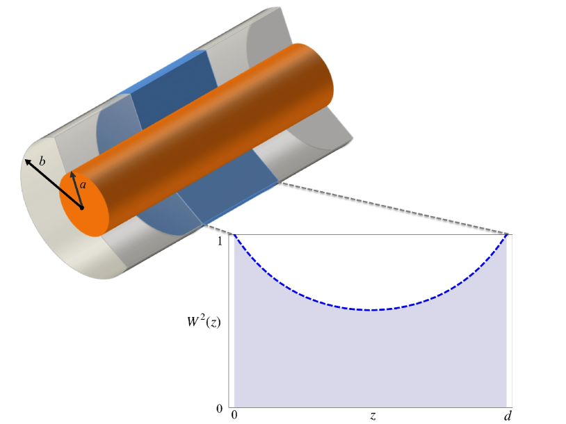
Figure 1:

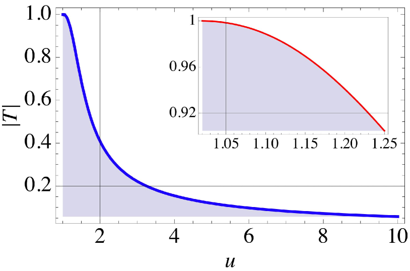
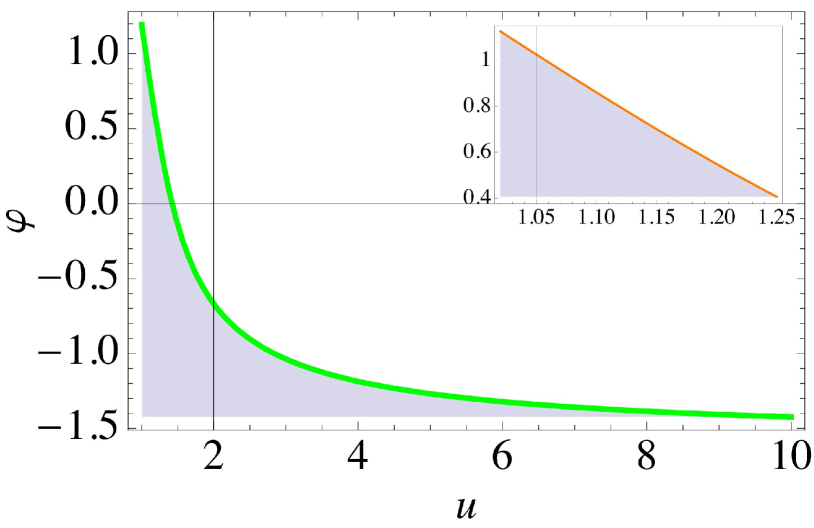
Figure 2:

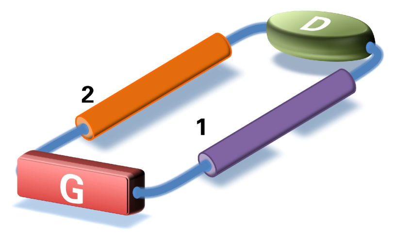
Figure 3:

References

- (1) G. A. Gamow, Zeits. f. Physik 51, 204 (1928).
- (2) R. W. Gurney and E. U. Condon, Nature 122, 439 (1928) ; Phys. Rev. 33, 127 (1929) .
- (3) T. E. Hartmann, J. Appl. Phys. 33, 3427 (1962);
- (4) R. Y. Chiao and A. M. Steinberg, Tunneling times and superluminality, Progress in Optics Vol XXXVII (Elsevier, New York, 1997) Ed. by E. Wolf.
- (5) M. Büttiker and S. Washburn, Nature 422, 271 (2003)
- (6) C.F. Li and Q. Wang, JOSA B 18, 1174 (2001).
- (7) D. Mugnai, A. Ranfagni and R. Ruggeri, Phys. Rev. Lett. 21, 4830 (2000).
- (8) V. S. Olkhovskya, E. Recamib and J. Jakielc, Phys.Rep. 398, 133 (2004).
- (9) M Büttiker and R Landauer, J. Phys. C: Solid State Phys. 21 6207 (1988).
- (10) A. M. Steinberg, P. G. Kwiat, and R. Y. Chiao, Phys. Rev. Lett. 71, 708 (1993).
- (11) A. B. Shvartsburg and G. Petite, Eur. Phys. J. D 36, 111 (2005)
- (12) A. B. Shvartsburg, V. Kuzmiak and G. Petite, Phys. Rev. E 76, 1127 (2006).
- (13) J. B. Pendry and D. R. Smith, Phys. Today 57, 37 2004 .
- (14) R. K. Wangsness, ”Electromagnetic fields” 2nd Ed. J. Wiley and Sons, NY (1986).
- (15) L. Stenflo, A. B. Shvartsburg and J.Weiland, Contrib. Plasma Phys. 37, 393, (1997).
- (16) R.W.Ziolkowsky, Phys. Rev. E 63, 046604 (2001).
- (17) G. Nimtz, Prog. Quant. Electron. 27, 417 (2003).