Embeddings of four-valent framed graphs into $2$-surfaces

Abstract

It is well known that the problem of defining the least (highest) genus where a given graph can be embedded is closely connected to the problem of embedding special four-valent framed graphs, i.e. 4-valent graphs with opposite edge structure at vertices specified. This problem has been studied, and some cases (e.g., recognizing planarity) are known to have a polynomial solution.

The aim of the following paper is to connect the problem above to several problems which arise in knot theory and combinatorics: Vassiliev invariants and weight systems coming from Lie algebras, Boolean matrices etc., and to give both partial solutions to the problem above and new formulations of it in the language of knot theory.

1 Introduction

We address the following question. Given a 4-valent graph $\Gamma$ with each vertex endowed with opposite half-edge structure.

A natural question is to study the highest (least) genus of the surface the graph can be embedded into. Of course, we mean only embeddings splitting the surface into $2$-cells. We shall address this general question later in this paper. First, we shall consider the following partial cases of it. One of them, more general, deals with embedded graphs whose first ${\bf Z}_{2}$-homology class is orienting. As a partial case of this, we address the following

Problem 1.

Which is the least possible (highest possible) genus of a $2$-surface $S$ this graph can be embedded into in such a way that the embedding represents the zero homology class in the surface (alternatively, the complement to the graph is checkerboard colourable).

Embeddings of such graphs representing the ${\bf Z}_{2}$-homology class are well studied for the case of the plane (see e.g., [LM, RR, Ma11]) and in the general case (see e.g., [LRS, CR]).

In fact, any embedding of a $4$-graph in ${\bf R}^{2}$ defines a checkerboard colouring on the set of faces because the plane has trivial first homology. On the other hand, any graph $\Gamma$ embedded into a $2$-surface $S$ (orientable or not) can be transformed into a $4$-graph by taking the medial graph $\Gamma^{\prime}$: the vertices of $\Gamma^{\prime}$ are the middle points of the edges of $\Gamma$, the edges of $\Gamma^{\prime}$ connect adjacent edges (sharing the same angle), and faces correspond to faces (white) and vertices (black) of $\Gamma$, see Fig. 1.

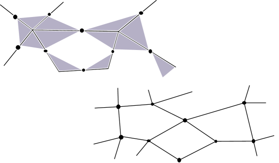
Figure 1: Any embedded graph generates a $4$-valent framed graph

Such $4$-valent graphs appeared with many names in different problems of low-dimensional topology: as atoms (see rigorous definition ahead), originally due to Fomenko [F], see the connection between atoms and knots in [Ma1], they are connected to Grothendieck’s dessins d’enfant, see [LZ] and [DFKLS].

There is a nice connection between combinatorics of Vassiliev invariants and other invariants of knots and virtual knots and many well-known functions on graphs, see [CDM] and references therein.

Finally, the genus of the atom (the genus of the checkerboard surface we are interested in) is closely connected to the estimates of the thickness for Khovanov and Ozsváth-Szabó homology for classical and virtual knots, see [Ma9] and [Low].

In [CR] there was a reformulation of the problem stated above in terms of ranks of some matrices.

We give another (very easy) formulation in terms of ranks of matrices which is closely connected to knot theory.

Problem 2.

Given a symmetric ${\bf Z}_{2}$-matrix $M$ of size $n\times n$, find a splitting of the set of indices $\{1,\dots,n\}$ into $I\sqcup J$ such that for the corresponding square matrices $M_{I}$ and $M_{J}$, the sum of ranks $rk(M_{I})+rk(M_{J})$ is minimal (resp., maximal).

This seems to be the easiest reformulation of the initial problem. Of course, we are looking for a solution which would either be fast (say, having polynomial time in the number of vertices) or connected to some interesting mathematical problems.

In knot theory, the study of classical knots is closely connected to the so-called $d$-digarams, chord diagrams with $2$ sets of pairwise unlinked chords (see rigorous definition ahead). It turns out that these diagrams play a special role in the chord diagram algebra having the highest possible degree of the Vassiliev invariants coming from $sl(n)$ (see [CM]). On the other hand, these are precisely those diagrams corresponding (in sense of [Ma1]) to planar $4$-valent graphs.

This is not incidental. In fact, the generating function for such embeddings is closely connected to the $sl(n)$-weight system, and latter sometimes gives estimates for the genus of the atom where the framed graph can be embedded into.

The paper is organized as follows. In the next section, we give the definitions of atom, chord diagram, $d$-diagram, virtual link and establish a connection between them and embedded graphs. We also give a proof of a conjecture due to Vassiliev (stated in [Vas2]) and proved in [Ma11] saying that the only obstruction to the planar embeddability of such graphs is the existence of two cycles with no common edges with exactly one transverse intersection point.

Later, we also give criteria for embeddability of framed graphs to the real projective space and in the Klein bottle.

In section 3, we define the Kauffman bracket for the virtual knots and we recall a result by Soboleva [Sob] about the number of circles which appear after a surgery along a chord diagram. This will lead us to the reformulation of Problem 1 as Problem 2.

Section 4 will be devoted to the connection between chord diagrams, weight systems and Vassiliev’s invariants coming from Lie algebras in sense of Bar-Natan [BN]. We shall prove a theorem giving an estimate in terms of $sl(n)$-invariants.

The last section will be devoted to the discussion and open problems.

1.1 Atoms and Knots

A four-valent planar graph $\Gamma$ generates a natural checkerboard colouring of the plane by two colours (adjacent components of the complement ${\bf R}^{2}\backslash\Gamma$ have different colours).

This construction perfectly describes the role played by alternating diagrams of classical knots. Recall that a link diagram is alternating if while walking along any component one alternates over- and underpasses. Another definition of an alternating link diagram sounds as follows: fix a checkerboard colouring of the plane (one of the two possible colourings). Then, for every vertex the colour of the region corresponding to the angle swept by going from the overpass to the underpass in the counterclockwise direction is the same.

Thus, planar graphs with natural colourings somehow correspond to alternating diagrams of knots and links on the plane: starting with a graph and a colouring, we may fix the rule for making crossings: if two edges share a black angle, then the we decree the left one (with respect to the clockwise direction) to form an overcrossing, and the right one to be an undercrossing, see Fig. 2. Thus, colouring a couple of two opposite angles corresponds to a choice of a pair of opposite edges to form an overcrossing and vice versa.

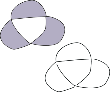
Figure 2: Surface colouring and a knot diagram

Now, if we take an arbitrary link diagram and try to fix the colouring of regions by colouring angles according to the rule described above, we see that generally it is impossible unless the initial diagram is alternating: we can just get a region on the plane where colourings at two adjacent angles disagree. So, alternating diagrams perfectly match colourings of the $2$-sphere (think of $S^{2}$ as a one-point compactification of ${\bf R}^{2}$). For an arbitrary link, we may try to take colours and attach cells to them in a way that the colours would agree, namely, the circuits for attaching two-cells are chosen to be rotating circuits, where we always turn inside the angle of one colour.

This leads to the notion of atom. An atom is a pair $(M,\Gamma)$ consisting of a $2$-manifold $M$ and a graph $\Gamma$ embedded $M$ together with a colouring of $M\backslash\Gamma$ in a checkerboard manner. Here $\Gamma$ is called the frame of the atom, whence by genus (resp., Euler characteristic) of the atom we mean that of the surface $M$.

Note that the atom genus is also called the Turaev genus, [Tu].

Certainly, such a colouring exists if and only if $\Gamma$ represents the trivial ${\bf Z}_{2}$-homology class in $M$.

Thus, gluing cells to some rotating circuits on the diagram, we get an atom, where the shadow of the knot plays the role of the frame. Note that the structure of opposite half-edges on the plane coincides with that on the surface of the atom.

Now, we see that atoms on the sphere are precisely those corresponding to alternating link diagrams, whence non-alternating link diagrams lead to atoms on surfaces of a higher genus.

In some sense, the genus of the atom is a measure of how far a link diagram is from an alternating one, which leads to generalisations of the celebrated Kauffman-Murasugi theorem, see [Ma1] and to some estimates concerning the Khovanov homology [Ma9].

Having an atom, we may try to embed its frame in ${\bf R}^{2}$ in such a way that the structure of opposite half-edges at vertices is preserved. Then we can take the “black angle” structure of the atom to restore the crossings on the plane.

In [Ma2] it is proved that the link isotopy type does not depend on the particular choice of embedding of the frame into ${\bf R}^{2}$ with the structure of opposite edges preserved. The reason is that such embeddings are quite rigid.

The atoms whose frame is embeddable in the plane with opposite half-edge structure preserved are called height or vertical.

However, not all atoms can be obtained from some classical knots. Some abstract atoms may be quite complicated for its frame to be embeddable into ${\bf R}^{2}$ with the opposite half-edges structure preserved. However, if it is impossible to immerse a graph in ${\bf R}^{2}$, we may embed it by marking artifacts of the embedding (we assume the embedding to be generic) by small circles.

This leads to a connection between atoms and virtual knots which perfectly agrees with virtual knot theory proposed by Kauffman in [Ka2].

Definition 1. A virtual diagram is a $4$-valent diagram in ${\bf R}^{2}$ where each crossing is either endowed with a classical crossing structure (with a choice for underpass and overpass specified) or just said to be virtual and marked by a circle.

Definition 2. A virtual link is an equivalence class of virtual link diagram modulo generalized Reidemeister moves. The latter consist of usual Reidemeister moves referring to classical crossings and the detour move that replaces one arc containing only virtual intersections and self-intersection by another arc of such sort in any other place of the plane, see Fig. 3.

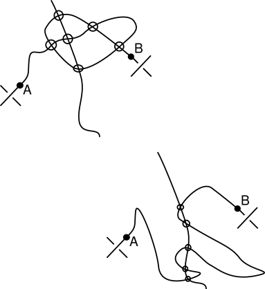
Figure 3: The detour move

Having freedom of immersing knot diagrams into ${\bf R}^{2}$ instead of just embedding, we are able to make virtual diagrams out of atoms. Obviously, since we disregard virtual crossings, the most we can expect is the well-definiteness up to detours. However, this allows us to get different virtual link types from the same atom, since for every vertex $V$ of the atom with four emanating half-edges $a,b,c,d$ (ordered cyclically on the atom) we may get two different clockwise-orderings on the plane of embedding, $(a,b,c,d)$ and $(a,d,c,b)$. This leads to a move called virtualisation.

Definition 3. By a virtualisation of a classical crossing we mean a local transformation shown in Fig. 4.

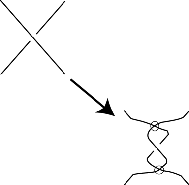
Figure 4: Virtualisation

The above statements summarise as

Proposition 1.

(see., e.g. [Ma1]). Let $L_{1}$ and $L_{2}$ be two virtual links obtained from the same atom by using different immersions of its frame. Then $L_{1}$ differs from $L_{2}$ by a sequence of (detours and) virtualisations.

Obviously, the inverse operation of obtaining an atom from a virtual diagram is well defined.

Note that many famous invariants of classical and virtual knots (Kauffman bracket, Khovanov homology, Khovanov-Rozansky homology [KhR1, KhR2]) do not change under the virtualisation, which supports the virtualisation conjecture: if for two classical links $L$ and $L^{\prime}$ there is a sequence $L=L_{0}\to\cdots\to L_{n}$ of virtualisations and generalised Reidemeister moves then $L$ and $L^{\prime}$ are classically equivalent (isotopic).

Note that the usual virtual equivalence implies classical equivalence for classical knots, see [GPV].

Definition 4. By a chord diagram we mean a cubic graph with a selected oriented cycle $S^{1}$ so that the remaining edges represent a collection of disjoint chords.

A chord diagram is called framed if every chord is marked by either $+1$ or $-1$. A chord diagram without framings is assumed to have all chords positive.

Two chords $A,B$ of a chord diagram are linked if the ends $A_{1}$ and $A_{2}$ of the first chord lie in different components of $S^{1}\backslash\{B_{1},B_{2}\}$.

Analogously, one defines a chord diagram on $m$ circles; there should be $m$ oriented cycles with some points connected by chords.

The intersection graph of a chord diagram is a graph whose vertices are in one-to-one correspondence with the edges of chord diagram and the vertices of the graph. Two vertices are connected by an edge iff the corresponding chords are linked.

A chord diagram (with all chords framed positively) is a $d$-diagram if the corresponding intersection graph is bipartite.

If the chord diagram is framed then the corresponding graph obtains framings at vertices.

Now, assume we have an atom with exactly one white cell. Then the whole information about the atom can be obtained from a rotating circuit along the boundary of this cell. Namely, consider a walk along this boundary (in any direction) as a map from $S^{1}$ to the atom, and connect the preimages of vertices of the atom by chords. We thus construct a framed chord diagram, where the framing is positive whence the orientations of the two two circles locally agree or negative otherwise, see Fig. 5.

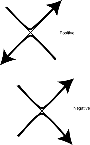
Figure 5: Two types of orientations in a neighbourhood of a vertex

From this chord diagram, one easily restores the atom and, thus, the corresponding virtual link up to detours and virtualisations.

Notation: For a chord diagram $C$ with one cell denote the corresponding atom by $A(C)$ and denote the corresponding virtual knot (considered up to detours and virtualisations) by $K(C)$.

1.2 Acknowledgements

I explain my gratitude for useful discussions to V.A.Vassiliev, A.T.Fomenko, L.H.Kauffman, S.K.Lando, S.V.Duzhin, S.V.Chmutov, O.M.Kasim-Zade, O.R. Campoamor-Stursberg.

2 Chord Diagrams, $1$-Dimensional Surgery and The Kauffman Bracket

The Kauffman bracket [Ka1] is a very useful model for understanding the Jones polynomial [Jon]. The Kauffman bracket associates with a virtual knot diagram a Laurent polynomial in one variable $a$ associated to every virtual diagram. After a small normalisation (multiplciation by a power of $(-a)$) it gives an invariant for virtual links.

This invariant can be read out of atom corresponding to a knot diagram. Namely, take an atom $V$ with $n$ vertices corresponding to a virtual diagram $L$ with $n$ classical crossings and call a state a choice of the couple of black or white angles at every vertex of $V$. Every such choice gives rise to a collection of closed curves on $V$ whose boundaries contain all the edges of $V$, see Fig. 6, and at each crossing the curves turn locally from one edge to an adjacent edge sharing the same angle of the prefixed colour.

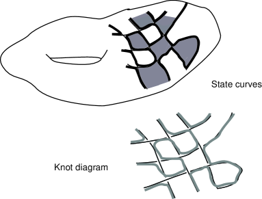
Figure 6: State curves drawn on an atom

Thus, having $2^{n}$ states of the atom, we define the Kauffman bracket of it as

$$\langle V\rangle=\sum_{s}a^{\alpha(s)-\beta(s)}(-a^{2}-a^{-2})^{\gamma(s)-1},$$ (1)

where the sum is taken over all states $s$ of the diagram, $\alpha(s)$ and $\beta(s)$ denote the number of white and black angles in the state (thus, $\alpha(s)+\beta(s)=n$ and $\gamma(s)$ denotes the number of curves in the state).

As it was said, the Kauffman bracket is invariant under the virtualisation. Thus, it is not surprising that it can be read out of the corresponding atom.

If the atom $A$ is obtained from a (framed) chord diagram $C$, then one can construct the Kauffman bracket $\langle C(A)\rangle$.

Thus, one obtains a function $f$ on framed chord diagram valued in Laurent polynomials in $a$. We shall return to that function because it is connected to the Vassiliev invariants of knots and $J$-invariants of closed curves (Lando, [Lando]).

Assume now we have a framed graph (a graph with each vertex labeled either positively or negatively).

By a rotating circuit of a framed graph $\Gamma$ we mean a map from the oriented circle $S^{1}\to\Gamma$ which is homeomorphic outside preimages of vertices of $\Gamma$, and each vertex of $\Gamma$ has precisely two preimages such that the corresponding neighbourhoods of them on the circle switch from one edge to an edge not opposite to it.

Every rotating circuit gives rise to a framed chord diagram associated with a graph: this chord diagram consists of the circle $S^{1}$ and chords connecting those points of $S^{1}$ having the same image in $\Gamma$. A chord is positive if for the corresponding vertex the two emanating edges are opposite.

Then it may or may not be represented as an intersection graph of a chord diagram (see [Bouchet] for the details) for which it is an intersection graph. Moreover, if such a chord diagram exists, it should not be unique, see, e.g., Fig. 7.

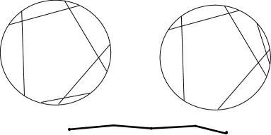
Figure 7: Two chord diagrams with the same intersection graph

This non-uniqueness usually corresponds to so called mutations of virtual knots.

The mutation operation (shown in the top of Fig. 8) cuts a piece of a knot diagram inside a box turn is by a half-twist and returns to the initial position.

It turns out that the mutation operation is expressed in terms of chord diagrams in almost the same way: one cuts a piece of diagram with $4$ ends and exchanges the top and the bottom part of it (see bottom picture of Fig. 8). Exactly this operation corresponds to the mutation from both Gauss diagram and rotating circuit points of view.

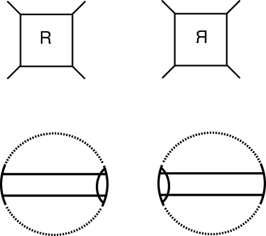
Figure 8: Mutation and its chord diagram presentation

In the bottom part of Fig. 8 chords whose end points belong to the “dotted” area remain the same; the other chords are reflected as a whole.

Regarded from the point of view of Gauss diagrams and the Vassiliev knot invariants, this non-uniqueness corresponds to mutations of classical links as well. Namely, S.K.Lando and S.V.Chmutov [ChL] proved the following

Theorem 1.

A Vassiliev invariant does not detect mutant knots if and only if the corresponding weight system depends only on the intersection graph of the chord diagram.

It is well-known that the Kauffman bracket does not detect mutations. Thus, one might guess that the corresponding Kauffman bracket can be read out of the intersection graph.

Surprisingly, the Kauffman bracket can be defined in a meaningful way even for those framed graphs which can not be represented as intersection graphs of chord diagrams.

Having a chord diagram, we can treat the states of the corresponding Kauffman bracket as collections of chords: we set the initial state $s_{0}$ to be empty collection of curves (with $\alpha(s)=n,\beta(s)=0$), and with each state $s$ we associate a collection of chords correpsonding to those vertices of the atom where $s$ differs from $s_{0}$.

Now, if we are able to calculate how many circles we have in each state, we can apply (1) to calculate the Kauffman bracket.

This can be seen from a chord diagram after introducing the notion of surgery along a chord.

Given a chord diagram $D$ on $n$ circles $C_{1},\dots,C_{n}$. Fix a chord $c$ of it. By surgery along $c$ we mean the following operation. We delete small neighbourhoods of endpoints of $c$ and connect the obtained endpoints by segments in the following way. There are $3$ ways of pairing the four points. One of them corresponds to the disconnection we have performing. We choose another way as follows. If $c$ is positive then we connect the endpoints according to the orientation of circles, and if $c$ is negative, we connect the endpoints in the way opposite manner, see Fig. 9

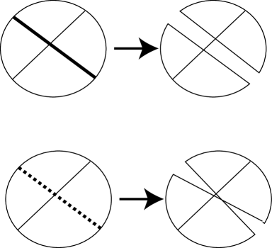
Figure 9: Surgeries along positive and negative chords

Then we get a collection of circles, not necessarily oriented. If we choose a collection of chords $c_{1},\dots,c_{k}$ of $C$, then the surgery along these chords means the consequence of surgeries performed along all chords $c_{i}$; in each case we look at the orientations of the initial diagram $C$.

Assume the circle represents a boundary component of an annulus. By adding a band to an annulus circle transforms its boundary component according to a surgery along the chord corresponding to the band, see Fig. 10.

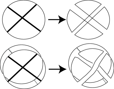
Figure 10: A surgery and its band representation

Thus, the number of circles in the state corresponding to the chords $d_{1},\cdots,d_{n}$ is precisely the number of components of the manifold obtained from the initial circle by surgery along these chords.

Now, for a framed graph $G$ on $k$ enumerated vertices, introduce the intersection matrix of $G$ to be $k\times k$ matrix over ${\bf Z}_{2}$ whose rows and columns correspond to vertices of $G$ such that $M_{ij}=M_{ji}=1$ for $i\neq j$ iff the vertices $i,j$ are connected by an edge and $M_{ii}=1$ iff $i$-th vertex is framed negatively.

Surprisingly, this number can be counted out of the intersection graph even when the corresponding chord diagram does not exist, due to the following

Theorem 2 (Soboleva,[Sob]).

For a chord diagram $D$ with an intersection graph $G$ the number of components of the manifold obtained from $D$ after a surgery along chords $1,\dots,k$ is one plus the corank of $M(D)$.

Now, we just define for a framed graph $\Gamma$ the Kauffman bracket as

$$\sum_{G^{\prime}\subset G}a^{2|G^{\prime}|-n}(-a^{2}-a^{-2})^{corankM_{\Gamma^{\prime}}}$$ (2)

Soboleva’s theorem allows to reformulate Problem 1 as Problem 2. Indeed, let $\Gamma$ be a framed $4$-graph. We are looking for an embedding of $\Gamma$ into a surface $S$ of minimal (maximal) genus with a checkerboard face colouring. Choose a rotating circuit of $\Gamma$ and a corresponding framed chord diagram $C(\Gamma)$.

Assume $\Gamma$ is embedded in a certain surface $S$. Then $C(\Gamma)$ yields a mapping $S^{1}\to S$ which is an embedding outside pre-images of vertices of $\Gamma$. This map can be slightly smoothed to give an embedding as shown in Fig. 11.

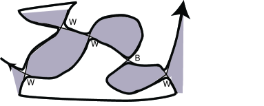
Figure 11: A circuit splits chords into two sets

Obviously, this circle $S^{1}\in S$ is separating: it divides the surface $S$ into the “white part” and the “black part”. We can draw all chords of $C(\Gamma)$ as small edges on $S$ lying in neighbourhoods of vertices of $\Gamma$. Thus, all chords of the chord diagram $C(\Gamma)$ are naturally split into two families: those connecting white regions and those connecting black regions.

Vice versa, any splitting of chords of $C(\Gamma)$ into two families (black and white) gives rise to a checkerboard colourable embedding of $\Gamma$ into a certain surface $S$. Indeed, consider an annulus $S^{1}\times I$ and let $S^{1}$ be the medial circle of this annulus. Now, we attach bands to two sides of the annulus according to the splitting; a band is overtwisted iff the corresponding chord is negative. This leads to a manifold $M$ with boundary; this boundary naturally splits into two parts corresponding to the boundary components of the annulus. Gluing the boundary components of $M$, we get the desired surface $S$ without boundary, see Fig. 12.

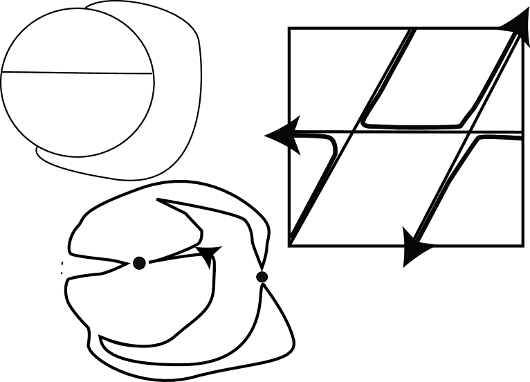
Figure 12: Restoring the atom from a chord diagram with two sets of chords

Thus, the question of estimating the genus (Euler characteristic) of $S$ is equivalent to the question of maximising (minimising) the boundary components of $S$. By definition, this is nothing but counting the number of components of the two $1$-manifolds obtained from the sphere by a surgery along the set of chords. By Soboleva’s formula, we have two subsets of chords $I$ and $J$, and we should take two coranks of the adjacency matrices $M_{I}$ and $M_{J}$.

Thus, we have to find a way of splitting the chords in order to maximise (minimise) the sum of ranks of the two matrices $rankM_{I}+rankM_{J}$.

Remark 1.

Note that this solution does not depend on a particular choice of a rotating circuit, depending only on the initial framed graph.

Statement 1.

Given a framed $4$-graph $\Gamma$ and the chord diagram $C(\Gamma)$ corresponding to some rotating circuit of $\Gamma$. Then if all chords of $C(\Gamma)$ are positive then all checkerboard colourable embeddings of $\Gamma$ yield orientable surface. If at least one chord of $\Gamma$ is negative then all such surfaces are non-orientable.

Remark 2.

Note that the statement above means, in particular, that if for some circuit the chord diagram contains a negative chord, then so are all diagrams corresponding to all rotating circuits for the same graph.

2.1 The source-target condition

The above condition can be reformulated intrinsically in the terms of graph.

Definition 5. We say that a four-valent framed graph satisfies the source-target condition if each edge of it can be endowed with an orientation in such a way that for each vertices some two opposite edges are emanating, and the remaining two edges are incoming.

Obviously, for a given graph there exists at most one source-target structure (up to overall orientation reversal of all edges). Moreover, if such a structure exists, then it agrees with any rotating circuit. Namely, starting with a rotating circuit one may try to orient its edges consequently in order to get a source-target structure of the whole framed graph. The only obstruction one gets in this direction corresponds to negative chords.

From the above, we get the following

Theorem 3.

A graph admits a source-target structure if and only if it is checkerboard-embeddable into an orientable surface; in other words, a source-target structure means that for any rotating circuit all chords are positive.

2.2 The planar case: Vassiliev’s conjecture

For a $4$-graph $\Gamma$ to be embedded in ${\bf R}^{2}$ (or $S^{2}$), take a chord diagram $C(\Gamma)$ corresponding to some rotating circuit of $\Gamma$, and consider the adjacency matrix $M_{C({\Gamma})}$. A simple calculation shows that the corresponding sum of ranks should be the minimal possible, i.e., equal to zero. That means that all chords of $\Gamma$ are positive (otherwise we would have diagonal non-zero entries giving rank at least $1$). Moreover, the chords should constitute two families of non-intersecting chords (each family forming a submatrix of rank $0$). This means that the corresponding intersection graph is bipartite or the diagram is a $d$-diagram.

Now, one can check that for a diagram with a negative chord $c$ there is a Vassiliev obstruction consisting of two circuits having precisely one intersection point at the vertex of $\Gamma$ corresponding to $c$. Besides, for a chord diagram which is not a $d$-diagram, one can explicitly construct a Vassiliev obstruct. This leads to a proof of Vassiliev’s conjecture. For more details see [Ma11].

Note that the above considerations lead to a fast (quadratic on the number of chords) algorithm of planarity recognition: one takes any circuit, checks whether all chords are positive, and then checks that a diagram is a $d$-diagram. The latter consists of possible splitting of all chords into two disjoint sets, which is unique for chord diagrams with connected intersection graphs.

2.3 The case of ${\bf R}P^{2}$

Here we shall use the adjacency matrix. According to Statement 1, the adjacency matrix should have at least one non-zero diagonal element. Without loss of generality, assume it is $(1,1)$. Since we are looking for a splitting of $\{1,\dots,n\}$ in order to get rank $1$, all elements entries $m_{jj}=1$ should belong to the same set. Without loss of generality, assume $a_{11}=\dots=m_{kk}=1,m_{k+1,k+1}=\dots m_{nn}=0$. Now, merge some subset $\{k+1,\dots,n\}$ with $\{1,\dots,n\}$ and leave the remaining part as it is in order to get the total rank $1$. The remaining part should thus have rank $0$, while the former should not increase rank $1$ formed by the first $k$ entries of the matrix. This can be done by the procedure similar to finding $d$-diagrams. The generic diagram corresponding to ${\bf R}P^{2}$ looks as follows (see Fig. 13): there is a family of dashed chords (all intersecting each other) and two families of pairwise disjoint chords; chords belonging to one family do not intersect dashed chords.

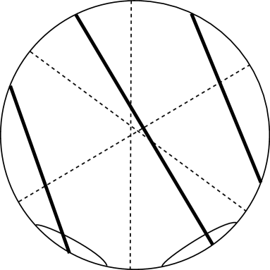
Figure 13: A generic framed chord diagram corresponding to a graph in ${\bf R}P^{3}$

In Fig. 13 solid chords from another family are represented by thicker lines than chords belonging to the family containing all dashed chords.

Obviously, the algorithm described in the present section has quadratic complexity.

2.4 The case of the Klein bottle

The main idea of detecting the Klein bottle embeddability is the following. While seeking the minimal rank $2$ there might be two possibilities: either $2=1+1$ (which corresponds to the Klein bottle represented as a connected sum of two projective planes or $0+0$; the first case is easier, and it turns out that the general case can be reduced to it).

Lemma 1.

For every four-valent framed graph embeddable in ${\bf KL}^{2}$ there exists a rotating circuit dividing ${\bf KL}^{2}$ into two copies of ${\bf R}P^{2}$.

Proof.

Starting with a rotating circuit bounding a disc, one can get a desired circuit by performing surgery along a dashed chord, see Fig. 14.

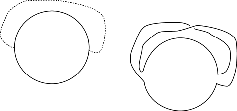
Figure 14: A surgery along a dashed chord generates a Möbius band

∎

Then, the procedure is as follows: we take a dashed chord, perform a surgery and look whether the intersection matrix corresponding to the obtained chord diagram is splittable into two families giving the desired decomposition.

The desired decomposition should be such that inside each family any two dashed chords intersect, and any non-dashed chord is disjoint from any other chord. Thus, the procedure of finding two families is exactly the same as in the case of $d$-diagrams, except for the case of incidence of dashed chords.

2.5 The chord diagram algebra and the graph algebra

Chord diagrams play a crucial role in the study of finite-type (Vassiliev) invariants of knots [Vas1, BN]. Roughly speaking, for every positive integer $n$ there is a class of invariants of degree $n$ whose “leading term” (called symbol or $n$-th derivative) is a function on chord diagrams satisfying a certain relation. Invariants of the same order having the same leading term differ by an invariant of a strictly smaller order (like polynomials of degree $n$ whose $n$-th derivative coincide).

There are two versions of the chord diagram algebra: for usual knots (with two sorts of relations, the four-term (see ahead) and the one-term) and for framed knots (with only the four-term relation).

We shall restrict ourselves for the case of only four-term relation which is defined as follows (see Fig. 15): given four diagrams on $n$ chords each whose $n-2$ chords coincide (they are not depicted in Fig. 15 and have endpoints in punctured areas) and the disposition of the remaining two chords, $\alpha$ and $\beta$ is as shown in Fig. 15.

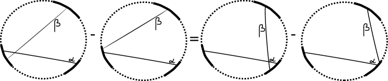
Figure 15: The four-term relation

Remark 3.

There exists a standard “deframing” procedure which associates with each weight system satisfying only the $4T$-relation a weight system satisfying both the $4T$ and the $1T$-relation. The latter means that the diagram containing a solitary chord is equal to zero.

We define the linear space ${\cal A}^{c}_{n}$ (over ${\bf Q}$) as the quotient space of all chord diagrams on $n$ chords modulo the four-term relation.

It turns out that the space ${\cal A}^{c}=\oplus_{i=0}^{\infty}{\cal A}^{c}_{n}$ has an algebra (and even bialgebra and Hopf algebra) structure. Namely, for multiplication of two chord diagrams we break each of them at some point and glue together with respect to the orientation. This operation is well-defined modulo $4T$-relation [Ma1].

The comultiplication operation for a chord diagram $C$ is defined as $\Delta(C)=\sum_{I\sqcup J}C_{I}\otimes C_{J}$, where the sum is taken over all possible ways to split the total set of chords into two subsets $I$ and $J$, and we take the subdiagrams $C_{I}$ and $C_{J}$ formed by these sets.

Having the intersection graph mapping, one can define the analogous operations on graphs. The multiplication operation is defined even easier than in the case of chord diagram: there is no need to prove its well-definiteness. On the other hand, one can define (following Lando, [CDL]) the $4T$-relation. It is defined as follows.

To make the definition of the graph algebra precise, we have to describe the correspondence between the $4$ terms $A,B,C,D$ in the graph-theoretic language. Since vertices of the graph correspond to chords, the diagrams $A$ and $B$ differ just by one chord: in $A$, the vertices $\alpha$ and $\beta$ are connected by an edge, whence for $B$ they are not. The same for $C$ and $D$. It remains only to explain how to get $C$ from $\alpha$. In the chord diagram we moved one end of the chord $\beta$ from one end of the chord $\alpha$ to the other while passing from $A$ to $C$, see Fig. 15. This means that the chord $\beta$ changes its incidence with all chords incident to $\alpha$ and does not change its incidence with chords which are not incident to $\alpha$.

Remark 4.

Note that the surgery over $A$ and the surgery over $C$ lead to the same number of circles; the same is true about $B$ and $D$.

It turns out that many nice functions defined on graphs (e.g., the Tutte polynomial) satisfy the $4T$-relation. We shall touch on such functions while defining the generating function for counting genera of surfaces spanning a given graph.

It turns out that the chord diagram algebra has its meaningful “framed analogue”. It is connected to so-called finite-type invariants of plane curves, see [Lando] for details. The definition goes as follows.

Consider the set of all framed chord diagrams on $n$ chords. Now, we set $A^{cf}_{n}$ to be the ${\bf Q}$-linear space generated by all such chord diagrams subject to the generalised $4T$-relations depicted in Fig. 16.

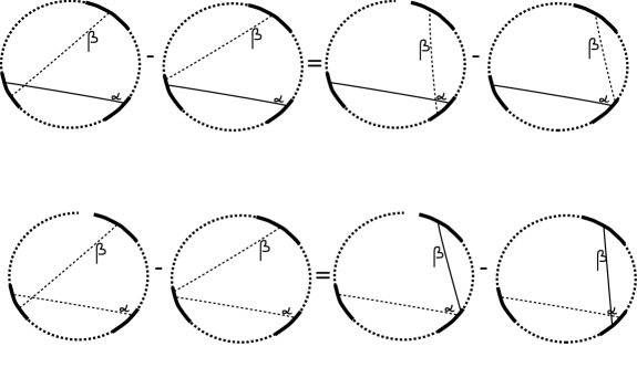
Figure 16: Two types of generalized 4-term relations

The general rule for the generalized four-term relation is as follows: we have $n-2$ fixed chords and two chords, $\alpha$ and $\beta$. If $\alpha$ is positive then in all chord diagrams $A,B,C,D$, the chord $\beta$ is of the same sign (in all cases positive or in all cases negative), and the relation looks just as the usual four-term relation: $A-B=C-D$. If $\alpha$ is negative, then while moving from $A,B$ to $C,D$ the chord $\beta$ changes its sign; moreover, the RHS changes the overall sign: $A-B=D-C$, that means that if in the LHS we take the chord diagram with intersecting $\alpha,\beta$ with plus then in the RHS we take the diagram with intersecting $\alpha,\beta$ with minus.

One can easily check that in any special case of the generalized $4T$-relation, the surgery along $A$ gives the same number of circles as the surgery along the diagram with plus in the right hand side ($C$ or $D$) whence the surgery along $B$ gives the same number of circles as the surgery along the diagram with minus from the RHS.

To the best of the author’s knowledge, the connected sum operation on the framed chord diagram algebra is not proved to be well-defined. Of course, the coalgebraic operation is well-defined.

Analogously, one defines the bialgebra of framed graphs (at the level of graphs, there is no problem to define the product, we omit the exact definition leaving it for the reader as an exercise).

3 The generating function for the embedding genera

3.1 Weight systems associated with Lie algebras: a brief review

There is a natural way of associating a number with a given chord diagram and a given representation of a (semisimple) Lie algebra due to Bar-Natan, [BN]. It turns out that the corresponding mapping naturally extends (for a fixed representation $R$ of a fixed Lie algebra $G$) to the mapping from the algebra of chord diagram ${\cal A}^{c}$ to ${\bf Q}$ because of the similarity of the $4T$-relation and the Jacobi identity.

We shall deal only with the adjoint representation of Lie algebras; for a Lie algebra $G$ we denote the corresponding mapping from ${\cal A}^{c}$ to ${\bf Q}$ by $W_{G}$.

The construction goes as follows. Every chord diagram is a cubic graph immersed in the plane with prefixed rotation direction at each vertex (when drawing chord diagrams on the plane we assume this rotation to be counterclockwise). We shall enlarge the construction for arbitrary cubic graphs with rotation. Namely, we take the structural tensor $L_{ijk}$ of the Lie algebra ${\bf G}$ with all indices shifted down by using the Cartan-Killing metric. Obviously, $L_{ijk}=L_{jki}=L_{kij}$. Now, we can associate with each trivalent vertex the tensor $L_{ijk}$ with indices corresponding to edges and going counterclockwise $i,j,k$. Then we contract all tensors along edges (of course, by using Cartan-Killing metric tensor) and get an integer.

We specify ourselves for the case of the Lie algebra $sl(n)$ and its adjoint representation.

In [Ma12], see also [CM], we proved the following

Theorem 4.

For a given chord diagram $D$ on $n$ chords, $W_{sl_{n}}(D)$ is a polynomial in $n$; its degree does not exceed $k+2$; moreover, it is equal to $k+2$ only in the case when $D$ is a $d$-diagram.

As an immediate consequence from this theorem we see that each basis of the chord diagram algebra consisting of chord diagrams contains at least one $d$-diagram.

On the other hand, it underlines the special role of $d$-diagrams amongst all chord diagrams from two points of view: as those (corresponding to graphs) embeddable in $S^{2}$ and as those having the highest possible degree of the leading term.

It turns out that this is not an incident: degrees of the $W_{sl_{n}}$ polynomial are closely connected to possible embeddings of the $4$-valent graph into surfaces. We shall touch on this subject in later sections.

3.2 Checkerboard colourable embeddings

As we have seen, in order to mimimise (maximise) the genus of the surface the graph can be embedded into, we have to maximise (minimise) the number of circles obtained as a result of surgeries along two subsets $I,J$ of chords of the initial chord diagram such that $I\sqcup J$ forms the complete set of chords.

Before we have reformulated this problem in terms of ranks of incidence matrices. A new formulation comes with the generating function.

Let $\Gamma$ be a framed $4$-valent graph on $k$ vertices, and let $D$ be a chord diagram corresponding to some circuit of $\Gamma$. Consider the following function

$$f(C):=f(\Gamma)=\sum_{atoms}x^{k+2-g},$$ (3)

where the sum is taken over all atoms with $A$-structure taken from $\Gamma$ and $g$ is the genus of the atom.

In view of Soboleva’s theorem, $f(C)$ depends merely on the intersection graph of $\Gamma$.

Consider the restriction of $f(C)$ to chord diagrams with only positive chords (i.e., to graphs corresponding to orientable atoms).

Theorem 5.

$f(C)$ is a well-defined function on the algebra of chord diagrams, i.e., it satisfies the $4T$-relation.

Analogously, $f(C)$ is a function on the graph algebra.

Moreover, $f(C)$ is multiplicative with respect to the multiplication operations in these algebras.

Both chord diagram algebra and graph algebra have a commutative and co-commutative Hopf-algebra structure, see, e.g., [BN, CDL, Ma1]. By Milnor-Moore theorem, [MM], each such algebra is isomorphic to the polynomial algebra of its primitive elements. Thus, in order to calculate $f(C)$ for a given chord diagram, one can use the algebraic structure of the Hopf algebra of chord diagrams (or graphs).

Now, we turn to the proof of Theorem 5. Consider a quadruple of chord diagrams $A,B,C,D$ on $n$ chords each forming a $4T$-relation $A-B=C-D$ as shown in Fig. 15. We can naturally identify chords from $A,B,C,D$: there are $n-2$ chords in common, one “fixed chord” (denoted by $\alpha$ in Fig. 15) and one “moving” chord (denoted by $\beta$).

Consider summands for $f(A),f(B),f(C),f(D)$ coming from the definition (3). For those summands where $\alpha$ and $\beta$ belong to the same subset of chords (say, $I$), the genus of surface corresponding to $A$ is equal to the genus corresponding to $C$, and the genus corresponding to $B$ is equal to the genus corresponding to $D$ (this follows from a straightforward calculation of the number of circles). Thus, these terms give the same contribution to (3).

For those summands where $\alpha$ and $\beta$ belong to different subsets $I$ and $J$, the corresponding subdiagrams coincide: $A_{I}=B_{I},A_{J}=B_{J},C_{I}=D_{I},C_{J}=D_{J}$ because when we move $\alpha$ and $\beta$ to different subdiagrams, it does not matter whether they intersect or not.

The proof for the graph algebra is analogous.

Arguing as above, one can prove the following

Theorem 6.

The restriction of function $f$ to ${\cal A}^{c}$ satisfies the generalised $4T$-relation.

Corollary 1.

If for a framed graph $\Gamma$ satisfying source-target condition on $k$ vertices and the corresponding chord diagram $C$ we have $degf(C)=k$ then $\Gamma$ is checkerboard-embeddable into torus.

Proof.

Indeed, the maximal possible degree $k+2$ corresponds only to planar embedding; the orienability of the surface is guaranteed by the source-target condition, and the degree $k$ corresponds to genus $1$. ∎

It is important to know what sort of weight system we obtain from $f$. It turns out that this weight system is closely connected to $W_{sl_{n}}$; roughly speaking, $W_{sl_{n}}$ can be represented as a sum of $2^{2k}$ summands (for $k$ chords); some $k$ of them give exactly the function $f$. Moreover, the $W_{sl_{n}}$-polynomial itself gives a “generating function” for some more general embeddings (see ahead), however, this generating function has signs $\pm$, so the embeddings are counted with pluses and minuses, which means that not the whole information can be restored from $W_{sl_{n}}$.

To clarify the situation, we shall need some more information about calculating $W_{sl_{n}}$ (see [Ma12] and [CM]). We will in fact work in $gl_{n}$; the result of final contraction will be the same as that for $sl_{n}$.

Given a chord diagram $D$, fix an arc of it and break this diagram along the arc. Then $W_{sl_{n}}(D)=Tr(x\to[\dots[,x]\dots]$ where by $[\dots[,]\dots]$ we mean the result of consequent commutators of $x$ with elements of the Lie algebra, where for each chord we take $\alpha$ on one end of the chord and the dual element $\alpha^{*}$ on the other end of the chord and sum up when $\alpha$ runs the basis of the Lie algebra. Let us be more specific. Consider the diagram shown in Fig. 17.

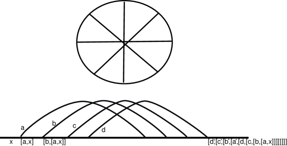
Figure 17: The contraction operator

The “long” commutator can be rewritten according to $[p,q]=pq-qp$. Thus we get $2^{2k}$ terms of the following form $(-1)^{l}p_{1}\dots p_{l}xq_{2k-l}\dots q_{1}$, where $p_{1},\dots p_{l}$ are variables corresponding to some chord ends in the usual order, and $q_{2k-l},\dots,q_{1}$ are the remaining chord ends in the reversed order. For instance, for a diagram shown in Fig. 17, we get summands like $(-1)d^{*}baxcda^{*}b^{*}c^{*}$.

Now, two simple $gl(n)$-contraction formulae come into play:

$$Tr(A\alpha B\alpha^{*})=Tr(A)Tr(B);\ Tr(A\alpha)Tr(B\alpha^{*})=Tr(AB).$$ (4)

Here the sum is taken over $\alpha$ running over a basis of $gl_{n}$, whence $\alpha^{*}$ runs the dual basis; $A$ and $B$ may be arbitrary $n\times n$ matrices.

With these formulae, we may contract any formula of the sort described above.

The formulae (4) have the following geometric meaning: if $A$ and $B$ represent collections of some chord ends (lying on one or two circles of a chord diagram) then the contraction transforms one circle into two or two circles into one.

This means precisely that the contraction rules in $sl_{n}$ correspond to surgery operations.

In the very beginning, we may contract $x$ with itself: this will lead to a subdivision of the circle into two circles according to the way of choosing variables on the left hand side with respect to $x$ and variables on the right hand side with respect to $x$.

Schematically, it means that we have to collect $2^{2k}$ terms corresponding to different splittings of chord ends into two circles. For instance, $(-1)d^{*}baxcda^{*}b^{*}c^{*}$ corresponds to the diagram shown in Fig. 18.

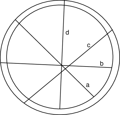
Figure 18: A chord diagram on 2 circles corresponding to $(-1)d^{*}baxcda^{*}b^{*}c^{*}$

Call a summand good if for each chord both ends belong to the same subset. Such summands contribute with sign $+$. Now, it follows from definition that the contribution of good summands gives exactly the function $f$.

Now, we the geometric meaning of the function $f$ itself.

3.3 Embeddings with orienting ${\bf Z}_{2}$-homology class

For generic summands (not necessarily good) we deal with arbitrary ways of splittings of chord ends into two sets. This leads to an arbitrary way of attaching bands to the annulus, and, finally, gives the generating function for arbitrary embeddings of our framed graph provided that the ${\bf Z}_{2}$-homology represented by this graph corresponds to an orienting cycle.

Let us be more specific. First of all, our weight systems corresponding to Lie algebras are defined only for the case when all chords of the chord diagram are positive. On the other hand, the generating function can be written down for an arbitrary graph. As we shall see, all generating functions will satisfy the generalized $4T$-relation and give a certain generalized weight system in the sense of Lando.

Analogously to $f$, we define the function ${\tilde{f}}$ as follows:

$${\tilde{f}}(C):={\tilde{f}}(\Gamma)=\sum_{{\bf Z}_{2}-\mbox{orient.emb}}x^{k+2-g},$$ (5)

where the sum is taken over ${\bf Z}_{2}$-orientable embeddings.

Analogously to Theorem 6, one can prove

Theorem 7.

The restriction of ${\tilde{f}}$ to chord diagrams satisfies the $4T$-relation.

This immediately yields the following

Corollary 2.

If ${\tilde{f}}(C)$ has maximal degree $k+2$ then the corresponding framed $4$-valent graph is checkerboard-embeddable into the torus.

Unfortunately, the inverse is not true: the graph corresponding to the chord diagram consisting of three pairwise-linked chords is embeddable into torus, though the $sl(n)$-function on this chord diagram gives zero.

Now, let us try to understand the geometric meaning of ${\tilde{f}}$. For a chord diagram on $k$ chords, the function $f$ can be represented by $2^{2k}$ summands which clearly correspond to some contraction rules in $sl_{n}$. These are exactly the summands corresponding to those contractions where we place both ends of each chord on the same circle.

It would be very interesting to understand the nature of contraction along chords connecting points on different circles, see Fig. (18).

First of all, in the expansion for a commutator, we may get a minus sign, which corresponds to a surgery along a chord diagram with two ends on different circles.

Now assume we perform count the $sl(n)$ weight system for a chord diagram. As we see, after expanding the commutators, the expressions for two circles go in the opposite order. Thus, in order to restore the real picture of embedding genera, one should perform overtwisted surgeries along chords with endpoints on different circles.

Thus, $W_{sl_{n}}$-weight system estimates the genera of the surfaces the graph can be embedded to, but:

1. It counts embeddings with signs, thus, for some embedding it does not give a real estimate for the genus. For instance, for the chord diagram with $3$ pairwise intersecting chords the value of the $W_{sl_{n}}$-function is zero.

2. The contraction corresponding to chords with ends on different circles count embeddings of the same graph, but with another framing.

So, the geometric meaning of ${\tilde{f}}$ is not yet completely understood.

3.4 The general case

We have described how to write the generating function of all embeddings for a given graph into surfaces such that the ${\bf Z}_{2}$-homology class of the graph is orienting.

Namely, let $\Gamma$ be a framed graph and let $C$ be its rotating circuit. If we want to embed $\Gamma$ into some surface in such a way that $\Gamma$ represents a non-orienting ${\bf Z}_{2}$-cycle then this condition depends on $\Gamma$ itself and does not depend on $C$. Thus, we have to start with embedding the neighbourhood of $C$ as the medial circle of the Möbius band. Then we attach bands to this Möbius band in the usual way (according to the $A$-structure of $\Gamma$) and paste the boundary components by discs.

At the level of chord diagrams this means the following. Instead of taking two copies of the chord diagram circle, we take a $2$-fold covering of the circle by a circle and distribute the $2n$ chord endpoints in one of two possible positions each, and then perform contraction, see Fig. 19.

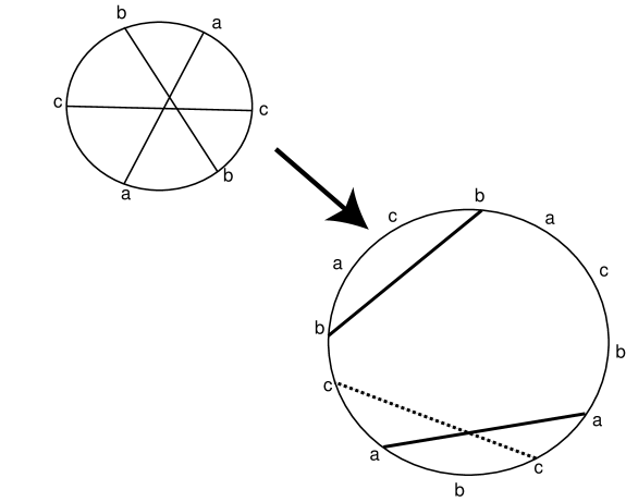
Figure 19: $2$-fold covering of a chord diagram

4 Unsolved problems

The method of matrix ranks gives an explicit polynomial solution only in a very limited number of cases. It is known that for every surface of rank $g$ there is a solution to Problem 1 which is polynomial in the number of chords. It would be very interesting to get such algorithms via matrices.

Both bialgebra of chord diagrams and coalgebra of framed diagrams are well known. At the level of chord diagrams their structures are well studied.

However, weight system approach is applicable only to chord diagrams with solid chords (which correspond to chord diagrams satisfying the source-target condition). It is not yet known how to apply any similar techniques for framed chord diagrams (with “dashed” chords). Possibly, one should treat positive chords by means of $sl(n)$-tensors, and negative chords by means of $so(n)$ or maybe $sp(n)$-tensors (cf. [BN] and [CM]).

It is well known (see [LZ]) that many enumerative problems in graph theory can be solved by using Gaussian integrals. However, these problems usually count generating functions for genera coming from all possible gluings, say, of a polygon. In our problem, we have to fix a graph (or a chord diagram), and consider the generating function for genera of surface this graph can be embedded into. Possibly, this can be done by means of a Gauss integral for all admissible gluings of crosses at vertices of the diagram.

A four-valent graph with $A$-structure can be represented as a shadow of a virtual link. Problem 1 is devoted to finding the minimal atom genus for a link with this shadow and some classical crossing setup. Fixing such a link with one white cell leads to a chord diagram and a rotating circuit. The Kauffman bracket of this link is very similar to the generating function for the solution of Problem 1: it has $2^{n}$ summands. It is known [Mel] that the Kauffman bracket (after some variable change) giving a series of weight systems integrates to give the Kauffman $2$-variable polynomial of the knot. It would be interesting to know which are the knot invariants that can be obtained by integrating the generating functions for Problem 1 and which knot-theoretic properties they can detect.

References

- [BN] Bar–Natan, D. (1995), On the Vassiliev Knot Invariants, Topology, 34, pp. 423 472.
- [Bouchet] Bouchet, A. (1994), Circle graph obstructions, J. Combinatorial Theory B, 60, pp. 107-144.
- [Bou] Bourgoin, M. O., Twisted Link Theory, arxiv: math. GT0608233
- [CDL] Chmutov, S.V., Duzhin, S.V., Lando, S.K. (1994), Vassiliev knot invariants , Advances in Soviet Math., 21, pp. 117-147.
-
[CDM]
S. Chmutov, S. Duzhin, Y. Mostovoy, CDBooK,
A draft version of the book about Vassiliev knot invariants.
http://www.math.ohio-state.edu/~chmutov/preprints/. - [CE1] G. Cairns and D. Elton, The planarity problem for signed Gauss words , J. Knot Theory Ramifications 2 (1993), 359 367.
- [CE2] G. Cairns and D. Elton, The planarity problem. II, J. Knot Theory Ramifications 5 (1996), 137 144.
- [ChK] Champanerkar, A., Kofman, I., Spanning trees and Khovanov homology, arxiv: math. GT0607510
- [ChL] Chmutov, S.V, Lando, S.K. (2007), Mutant knots and intersection graphs, arxiv. math: GT 0704.1313
- [CM] Campoamor-Stursberg, R., Manturov, V.O. (2004), Invariant tensors formulae via chord diagrams, Journal of Mathematical Sciences, 128, N.4, pp. 3018-3029.
- [CR] Crapo, H., Rosenstiel, P., On lacets and their manifolds, Discrete Mathematics 233 (2001) 299 320.
- [DFKLS] Dasbach, O., Futer, D., Kalfagianni, E., Lin, X.-S., Stoltzfus, N.(2006), The Jones Polynomial and Graphs on Surfaces, arXiv.math/Gt:0605571v3.
- [Dro] Drobotukhina Yu.V. (1991), An Analogue of the Jones-Kauffman poynomial for links in and a generalisation of the Kauffman-Murasugi Theorem, Algebra and Analysis, 2(3), pp. 613-630.
- [DK2] Dye, H.A., Kauffman, L.H. (2004), Minimal Surface Representation of Virtual Knots and Links, arXiv:math. GT/0401035 v1.
- [F] Fomenko A. T. (1991), The theory of multidimensional integrable hamiltonian systems (with arbitrary many degrees of freedom). Molecular table of all integrable systems with two degrees of freedom, Adv. Sov. Math, 6, pp. 1-35.
- [FKM] Fenn, R.A, Kauffman, L.H, and Manturov, V.O. (2005), Virtual Knots: Unsolved Problems, Fundamenta Mathematicae, Proceedings of the Conference “Knots in Poland-2003”, 188.
- [GPV] Goussarov M., Polyak M., and Viro O.// Topology. 2000. V. 39. P. 1045–1068.
- [JKS] Jaeger, F., Kauffman, L.H., and H. Saleur (1994), The Conway Polynomial in and Thickened Surfaces: A new Determinant Formulation, J. Combin. Theory. Ser. B., 61, pp. 237-259.
- [Jon] Jones, V. F. R. (1985), A polynomial invariant for links via Neumann algebras, Bull. Amer. Math. Soc., 129, pp. 103-112.
- [Ka1] Kauffman, L.H., (1987), State Models and the Jones Polynomial, Topology, 26, pp. 395–407.
- [Ka2] Kauffman L.H., Virtual knot theory, Eur. J. Combinatorics. 1999. V. 20, N. 7. P. 662-690.
- [Kh] Khovanov, M. (1997), A categorification of the Jones polynomial, Duke Math. J,101 (3), pp.359-426.
- [KhR1] Khovanov, M., Rozansky, L., Matrix Factorizations and Link Homology, Arxiv.Math:GT/0401268
- [KhR2] Khovanov, M., Rozansky, L.,Matrix Factorizations and Link Homology II, Arxiv.Math:GT/0505056
- [KK] Kamada, N. and Kamada, S. (2000), Abstract link diagrams and virtual knots, Journal of Knot Theory and Its Ramifications, 9 (1), pp. 93–109.
- [Kup] Kuperberg, G. (2002), What is a Virtual Link?, www.arXiv.org, math-GT0208039, Algebraic and Geometric Topology, 2003, 3, 5 87-591.
- [Lando] Lando, S.K. (2006), -invariants of ornaments and framed chord diagrams, Functional Analysis and Its Applications, 40 (1), pp. 1-13.
- [LM] L. Lovász and M. Marx, A forbidden substructure characterization of Gauss codes , Acta Sci. Math. (Szeged) 38:1 2 (1976), 115 119.
- [LZ] Lando, S.K., Zvonkine, A.K., Embedded Graphs, Springer, 2003.
- [Lee] Lee, E.S. (2003) On Khovanov invariant for alternating links, arXiv: math.GT0210213.
- [Low] Lowrance, A. On Knot Floer Width and Turaev Genus, (2007),arXiv: math.GT709.0720v1
- [LRS] Lins, S., Richter, B., Schank, H. (1987), The Gauss Code Problem off the plane, Aequationes Mathematicae, pp. 81-95.
- [Ma1] Manturov, V.O., Teoriya Uzlov (Knot Theory, In Russian), RCD, M.-Izhevsk, 2005.
- [Ma2] Manturov, V.O. (2000), Bifurcations, Atoms, and Knots, Moscow Univ. Math. Bull. 1, pp.3–8.
- [Ma3] Manturov, V.O. (2004), The Khovanov polynomial for Virtual Knots, Russ. Acad. Sci. Doklady, 398, N. 1., pp. 11-15.
- [Ma4] Manturov V.O. (2006), The Khovanov Complex and Minimal Knot diagrams, Russ. Acad. Sci. Doklady, 406, (3), pp. 308-311.
- [Ma5] Manturov V.O. (2005), The Khovanov complex for virtual knots, Fundamental and applied mathematics, 11, N. 4., pp. 127-152 (in Russian).
- [Ma6] Manturov V.O. (2005), On Long Virtual Knots, Russ. Acad. Sci. Doklady, 401 (5), pp. 595-598.
- [Ma7] Manturov V.O. (2007), Khovanov Homology for Virtual Knots with Arbitrary Coefficients, Russ. Acad. Sci. Izvestiya, 71, N. 5, pp. 111-148.
- [Ma8] Manturov V.O. (2007) Additional gradings in the Khovanov Complex for Thickened Surfaces, Russ. Acad. Sci. Doklady, to appear.
- [Ma9] Manturov, V.O., Minimal diagrams of classical knots, ArXiv:GT 0501510.
- [Ma10] Manturov, V.O. (2003), Kauffman–like polynomial and curves in –surfaces, Journal of Knot Theory and Its Ramifications, 12, (8), pp.1145-1153.
- [Ma11] Manturov, V.O. (2004), The proof of Vassiliev’s conjecture on planarity of singular graphs.
- [Ma12] Manturov, V.O. (2002), Chord diagrams and Invariant Tensors, Proceedings of the 1 Colloquium on Lie Theory and Applications, pp. 117-125.
- [Mel] Mellor, B. (2000), Three weight systems arising from intersection graphs, arXiv.math/Gt:0004080v1.
- [MM] Milnor, J., Moore, J. (1965), On the Structure of Hopf Algebras, Ann. Math., pp. 211-264.
- [RR] Rosenstiel, P. and Read, R., On the principal edge tripartition of a graph, Ann. Discrete Math 3 (1978)
- [Sob] Soboleva, E. (2001), Vassiliev Knot Invariants Coming from Lie Algebras and -Invariants, Journal of Knot Theory and Its Ramifications, 10 (1), pp. 161-169.
- [Tu] V. Turaev, A simple proof of the Murasugi and Kauffman theorems on alternating links, L’Enseignement Mathématique 33 (1987) 203–225.
- [Vas1] Vassiliev, V. A. (1990), Cohomology of knot spaces, in Theory of Singularities and its applications, Advances in Soviet Mathematics,1, pp. 23–70.
- [Vas2] Vassiliev, V.A. (2005), First-order invariants and cohomology of spaces of embeddings of self-intersecting curves in , Izvestiya Mathematics, 69 (5), pp. 865-912.
- [Viro] Viro, O., Virtual links and orientations of chord diagrams, Proceedings of the Gökova Conference-2005, International Press, pp. 187-212.
- [Weh] Wehrli, S.,A spanning tree model for Khovanov homology, arxiv: math. GT0409328