Chaotic Advection and the Emergence of Tori in the Küppers-Lortz State

Abstract

Motivated by the roll-switching behavior observed in rotating Rayleigh-Bénard convection, we define a Küppers-Lortz (K-L) state as a volume-preserving flow with periodic roll switching. For an individual roll state, the Lagrangian particle trajectories are periodic. In a system with roll-switching, the particles can exhibit three-dimensional, chaotic motion. We study a simple phenomenological map that models the Lagrangian dynamics in a K-L state. When the roll axes differ by $120^{\circ}$ in the plane of rotation, we show that the phase space is dominated by invariant tori if the ratio of switching time to roll turnover time is small. When this parameter approaches zero these tori limit onto the classical hexagonal convection patterns, and, as it gets large, the dynamics becomes fully chaotic and well-mixed. For intermediate values, there are interlinked toroidal and poloidal structures separated by chaotic regions. We also compute the exit time distributions and show that the unbounded chaotic orbits are normally diffusive. Although the map presumes instantaneous switching between roll states, we show that the qualitative features of the flow persist when the model has smooth, overlapping time-dependence for the roll amplitudes (the Busse-Heikes model).

1 Introduction

In this paper, we study the motion of a passive tracer in two simple kinematic models of the Küppers-Lortz instability, a classical problem in rotating convection. Each model is composed of sequentially acting rolls whose axes lie in a plane and are rotated by $120^{\circ}$. In the limit when the switching from roll to roll is rapid, the tracer trajectories limit onto a classical hexagonal convection pattern. As the switching time increases, tracer trajectories predominately lie on two-dimensional tori. Eventually, these tori are destroyed and the dynamics becomes chaotic and strongly mixing.

The mixing of tracer elements in a flow is due to a combination of stirring and diffusion. While stirring rapidly transports the tracers by kinematic advection, the associated stretching and folding of material lines and surfaces ultimately triggers diffusive processes that homogenize the tracers into a blended mixture. Despite this relatively simple description, a complete understanding of the spatial and temporal evolution of tracer elements in a given flow remains a mathematically challenging problem [1]. This is further compounded if the tracers are not passively advected, but nonlinearly interact with fluid flow and perhaps other species. The phenomena of mixing is fundamentally important in many physical and engineering applications and it occurs at a variety of scales ranging from the very small (micrometer scale) to the very large (planetary scales and beyond). For instance, mixing in microchannels can be used to efficiently homogenize reagents in chemical reactions even when the flow is laminar [2]. In reaction-diffusion and combustion systems, the efficiency of mixing reactive agents is a crucial factor. Understanding transport for planetary scale flows is critical for climate modeling and pollution dispersion in atmospheric science [3] and eddy dynamics in oceanography [4].

While mixing is prominent in turbulent flows, effective mixing also occurs in laminar flows that have chaotic Lagrangian trajectories. The innovative work of Aref [5] gave birth to the subject of chaotic advection, which provides a mathematical foundation for investigating mixing and transport from a dynamical systems perspective [6]. Aref called his seminal model the “blinking vortex;” it was specifically designed to yield nonintegrable Lagrangian trajectories. This model can be interpreted as an idealized mixing protocol where passive tracers are successively captured by the velocity fields of vortical stirrers that are the analogues of turbulent eddies with finite lifetimes.

Recently, several models for three-dimensional Lagrangian dynamics have been constructed out of vortical roll arrays. Transport in a set of orthogonal, time independent roll arrays was investigated in [7, 8]. In this system long-range, superdiffusive transport only occurs along the direction perpendicular to the axes of both rolls. This flow could be realized using a combination of thermal convection and magnetohydrodynamic forcing.

In a previous paper, we studied motion in a set of rolls whose axes are orthogonal, and whose amplitudes oscillate [9]. This models the oscillations observed in experiments on convection in binary fluids [10]. The experiments showed that the convective instability gives rise to a sequence of temporally alternating, orthogonal roll arrays whose axes are parallel to the square boundaries. The transition from one set of rolls to the other was observed to be rapid, so that much of the time the fluid is dominated by a single set of parallel rolls. In our model, regardless of the choice of temporal dependence of the roll amplitudes, the Lagrangian dynamics is restricted two-dimensional surfaces; consequently, our model does not lead to three-dimensional mixing, though the two-dimensional dynamics can be chaotic. Our model contrasts with that of [7, 8] in that their rolls are $90^{\circ}$ out of phase.

Roll-switching was predicted for rotating convection in thin fluids by Küppers and Lortz [11, 12]. Here a thin fluid layer of large horizontal extent (i.e. small aspect ratio) is rotated about its vertical axis. When the rotation rate is small, a stationary roll pattern forms at a critical Rayleigh number. Above a critical rotation rate this pattern becomes unstable to a second set of two-dimensional rolls whose axes are rotated with respect to the original roll axes by some “switching angle,” $\Theta$. These rolls grow, causing the first set to decay. The secondary rolls then lose stability to a new set of rotated rolls and the process repeats.

This behavior has been observed in a variety of experiments [13]. Typically the weakly supercritical regime shows large patches of homogeneous rolls that loose stability to rolls with an axis rotated by a switching angle that varies with the Taylor and Prandtl numbers. For example in water (Prandtl number near seven), $\Theta=63\pm 3^{\circ}$ [14]. Theoretical investigations confirm the dependence of $\Theta$ on rotation rate, boundary conditions, and Prandtl number [15, 16]. Though the time dependence of the roll switching is not observed to be precisely periodic, there is a mean switching frequency that decreases as the Taylor number increases, but increases with the Rayleigh number [17].

Motivated by these experiments, we call three-dimensional fluid flow consisting of a set of rolls with different axes, whose amplitudes oscillate a Küppers-Lortz state. In this paper we analyze a simple model of the Lagrangian trajectories in a Küppers-Lortz state. We begin in §2 by constructing a time-dependent model with a simple spatial roll structure. When the switching is much faster than the roll turnover time, it can be idealized as instantaneous and the flow can be viewed as a composition of volume-preserving maps corresponding to the action of each individual roll. This gives rise to what we call a blinking roll model in §3; it is analogous to Aref’s blinking vortex model. To check the importance of the assumption of instantaneous switching, we also introduce in §4 a continuous model using the Busse-Heikes system of odes for the evolution of the roll amplitudes [18, 19]. When the switching angle $\Theta$ is $120^{\circ}$ or $60^{\circ}$ symmetry, as reviewed in §5, allows us to restrict our analysis to a fundamental hexagonal cell. Finally, in §6, computational results are discussed and mixing is analyzed using Lyapunov exponents and anomalous diffusion exponents [20].

Even when some three-dimensional mixing occurs in these models, it is usually not complete because there are families of two-dimensional invariant tori that form barriers to the Lagrangian trajectories. Such families of tori are prominent in three-dimensional, incompressible flows; they play a roll analogous to that of invariant closed curves in two-dimensional, area-preserving mappings [21]. Tori have also been experimentally observed, for example, in a cylindrical container with a tilted stirrer [22, 23]. These are visualized with sheet lasers and fluorescent dyes and correlate closely with corresponding island chains of the Poincaré sections of a model flow. Similar tori have also been seen for weakly buoyant tracers in a laminar flow [24]. We investigate some of the behavior of the families of tori in our system in §6.

2 Küppers-Lortz Roll Model

For the purpose of making progress analytically, we use the simplest roll model for rotating convection: the linearized solutions in the Boussinesq approximation with stress-free boundary conditions [25]. These rolls are tilted by an angle $\eta$ due to the Coriolis force. In scaled coordinates with the fluid confined to $z\in[\pi/2,\pi/2]$, the roll velocity field is

$$\mathbf{u}_{\eta} = A\left(-\tan(\eta)\sin(y)\sin(z),-\sin(y)\sin(z),-\cos(y)\cos(z)\right)\;.$$ (1)

Here, $A$ is the amplitude of the rolls and

$$\tan(\eta)=\frac{\tau}{k_{c}^{2}+\pi^{2}}\;,$$ (2)

where $\tau$ denotes the Taylor number and $k_{c}$ is the critical wave number at the onset of convection. For highly viscous flows and infinite Prandtl number, roll switching starts at a Taylor number $\tau_{c}=54.8$ with $k_{c}=3.95$, so that $\eta\approx 65^{\circ}$ . When the thin fluid layer is not rotating, $\tau=\eta=0$, and the velocity field simplifies to:

$$\mathbf{u}_{0}=A\left(0,-\sin(y)\sin(z),-\cos(y)\cos(z)\right)$$ (3)

Although a rigid lower boundary together with a free upper surface is more physical (in which case Chandrasekhar functions would be the appropriate building block [25]), this choice would complicate both the analytical and numerical treatment. Moreover, in the limit $\tau\gg 1$, it has been shown [26, 27] that the stress-free solutions converge to the rigid ones outside the passive $\mathcal{O}(\tau^{-\frac{1}{2}})$ Ekman boundary layers.

Trajectories of (1) are confined to two-dimensional contours about axes parallel to $\hat{e}_{1}$ (the $x$-axis). A Küppers-Lortz state can be modeled in a simple way by using the roll solutions (1) as the building blocks of the flow. Our model is a superposition of rolls with amplitudes $A_{j}(t)$ whose axes are rotated by angles that are multiples of $\Theta$:

$$\mathbf{u}(\mathbf{x},t)=\sum_{j=0}^{N-1}A_{j+1}(t)R\left(j\Theta\right)\mathbf{u}_{\eta}\left(R^{T}(j\Theta)\mathbf{x}\right)\;.$$ (4)

Here $R$ is the rotation about the $z$-axis by an angle $\Theta$:

$$R(\Theta)=\left(\begin{matrix}\cos(\Theta)&-\sin(\Theta)&0\cr\sin(\Theta)&\cos(\Theta)&0\cr 0&0&1\end{matrix}\right)\;.$$ (5)

Since each individual roll is incompressible, any composition with arbitrary time-dependence is also incompressible.

We will assume that the rolls act sequentially. That is, when the $j^{th}$ roll is active, the amplitudes of all other rolls are nearly zero, and that as $t$ increases, $A_{j}(t)$ decreases to zero, and the next roll $A_{j+1}(t)$ activates and so forth.

If $\frac{\Theta}{2\pi}=\frac{p}{q}$ is rational, then it is appropriate to set $N=q$, since if the $j^{th}$ roll looses stability to the $(j+1)^{st}$ roll, then the whole process starts over after $q$ steps. If, however, $\frac{\Theta}{2\pi}$ were irrational, then the instability would continue to generate rolls at angles $j\Theta$, and the the “number” of rolls, $N$ would be effectively infinite.

The simplest case of (4) corresponds to $N=2$ and to orthogonal rolls, as we studied in [9]. Here we will study the case $N=3$ and a switching angle $\Theta=2\pi/3$. Letting

$$R\equiv R(2\pi/3)$$

we then have the velocity field

$$\mathbf{u}_{T}(\mathbf{x},t)=A_{1}(t)\mathbf{u}_{\eta}(\mathbf{x})+A_{2}(t)R\mathbf{u}_{\eta}(R^{T}\mathbf{x})+A_{3}(t)R^{T}\mathbf{u}_{\eta}(R\mathbf{x})\;;$$ (6)

Note that this model corresponds to a switching angle of $120^{\circ}$, not $60^{\circ}$. However, we shall see in §5 that the roll (1) has a reflection symmetry through the origin in the $xy$ plane, thus these two are equivalent.

When the amplitudes are constant and equal, this velocity field gives the (rotating) classical hexagonal convection cell

$$\mathbf{u}_{h}(\mathbf{x})=\mathbf{u}_{\eta}(\mathbf{x})+R\mathbf{u}_{\eta}(R^{T}\mathbf{x})+R^{T}\mathbf{u}_{\eta}(R\mathbf{x})\;,$$ (7)

The orbits of this autonomous system are either periodic or heteroclinic connecting equilibria on the upper and lower boundaries [25].

3 The Blinking Roll Map

The simplest model of sequential rolls corresponds to roll amplitudes that are periodic step functions. Motivated by the experiments, as well as by simplicity, we assume that both the strength and the the activation time of each roll is the same. In this case we can rescale time, setting $At\to t$ so that the roll amplitudes become one. The scaled roll activation time, $T$, thus represents both the strength and period of the flow. In this case the roll amplitudes are

$$A_{j}(t)=\left\{\begin{array}[]{ll}1,&\mbox{ for }(j-1)T\leq t<jT\;,\cr 0,&\mbox{ otherwise}\end{array}\right.\;.$$ (8)

for $0\leq t<NT$ and periodically repeating thereafter.

When the amplitude is constant, the flow for the vector field (3) can be solved exactly in terms of Jacobi elliptic functions. To get the flow for the tilted roll, we use the $\eta=0$ solutions of [9] and note note that in (1), $\dot{x}=\tan(\eta)\dot{y}$, giving

$$\Phi_{t}(\mathbf{x})=\left(\begin{array}[]{c}x+\tan(\eta)\left[\text{sgn}(y)\cos^{-1}\delta-y\right]\\ \text{sgn}(y)\cos^{-1}\delta\\ \sin^{-1}\chi\end{array}\right)\;,$$ (9)

where

$$\delta(y,z,t) \equiv\frac{\cos(y)\text{cn}(t)\text{dn}(t)+\text{sn}(t)\sin(z)\sin^{2}(y)}{1-\cos^{2}(y)\text{sn}^{2}(t)}\;,$$

$$\chi(y,z,t) \equiv\frac{\sin(z)\text{cn}(t)\text{dn}(t)-\text{sn}(t)\cos(y)\cos^{2}(z)}{1-\sin^{2}(z)\text{sn}^{2}(t)}\;,$$

and the elliptic functions have modulus

$$k=\sqrt{1-\sin^{2}y\cos^{2}z}\;.$$ (10)

By setting $t=T$ in (9), we get the time-$T$ map

$$F(\mathbf{x})=\Phi_{T}(\mathbf{x})\;.$$ (11)

The effective map for the other rolls can be obtained from (11) by rotation. For example in the three-roll case the resulting mapping is

$$f =(R\circ F)^{3}\;.$$ (12)

The map $f$ corresponds to the flow of (6) over the time $3T$. Note that since the vector field is incompressible, the map $f$ is volume preserving. Thus, the determinant of the Jacobian, $Df$, is equal to one.

Different values of $\Theta$ can can be easily accommodated by the map by replacing $R$ with $R(\Theta)$. When $\frac{\Theta}{2\pi}$ is irrational, we simply repeatedly iterate $R(\Theta)\circ F$.

4 Continuous-Time Models

One simple model of the temporal dependence of the amplitudes of three rolls is the Busse and Heikes model [18],

$$\dot{A}_{1} =A_{1}(1-|A_{1}|^{2}-\alpha|A_{2}|^{2}-\beta|A_{3}|^{2})$$

$$\dot{A}_{2} =A_{2}(1-|A_{2}|^{2}-\alpha|A_{3}|^{2}-\beta|A_{1}|^{2})$$ (13)

$$\dot{A}_{3} =A_{3}(1-|A_{3}|^{2}-\alpha|A_{1}|^{2}-\beta|A_{2}|^{2})\;.$$

When $\alpha$ and $\beta$ are positive, this system has a heteroclinic cycle between three states. This model could also include evolution of the phases of the rolls, but we assume that these are constant.

A thorough review of the dynamic properties of (4) is given in [19]. When $\alpha>1>\beta$, there exists an attracting heteroclinic cycle connecting the saddle equilibria, i.e. the pure roll states: $(A_{1},A_{2},A_{3})=(1,0,0)$, $(0,1,0)$, and $(0,0,1)$. The presence of the attracting equilibria yields a system that spends increasing amounts of time around the unstable roll states. This feature is not physical, since experimental observations suggest a characteristic period of oscillation associated with a Küppers-Lortz state. Busse and Heikes offered several ideas for overcoming this problem. One proposal involves the introduction of small amplitude noise into (4) designed to simulate the missing terms in the true amplitude equations. Noisy perturbations of attracting heteroclinic cycles were first studied in [28]. Perturbations of this type prevent the system from spending increasing amounts of time about any one of the saddle equilibria [19]. The noisy system has a statistically “stable” limit cycle with a well-defined mean period. A second suggestion is to add slow spatial variation to the amplitude [29]. Adding terms of form $\partial^{2}_{x_{i}}A_{i}$ to each equation in (4) respectively also creates a stable oscillation, although its period is difficult to predict.

We implement the stochastic method by adding the derivative of small white noise terms, $\xi_{i}(t)$, to (4). Specifically, the $\xi_{i}(t)$ are Wiener processes with mean $2\epsilon$ and variance $\epsilon^{2}$. The mean is nonzero to help avoid pushing the amplitudes out of the positive octant . Time series are obtained using a second-order stochastic Runge-Kutta solver [30, 31]. Noise causes the orbit to be pushed away from the unstable single roll solutions, preventing it from spending arbitrarily long durations near any of those states.

Detailed pictures of the asymptotically periodic evolution are shown in Fig. 1. The model has three parameters $\alpha$, $\beta$, and $\epsilon$ that can be chosen to control mean period, shape, and symmetry of the amplitude waveforms. The curves in Fig. 1a and c show typical realizations of the amplitude evolution; the solid curves correspond to much smaller values of $\epsilon$ than the dashed curves . In Fig. 1b and d, probability distribution functions (PDFs) of the periods are shown. For the first case the mean period, $\tau_{\text{switch}}$ is close to $1.5$, while in the second it is close to $3$. For each case, a step size, $\Delta t$, was chosen so that there were roughly $300$ steps per period. The PDFs were computed using $\sim 10^{5}$ periods of a single realization. In both cases, the probability distribution functions for the period appear to be nearly Gaussian.

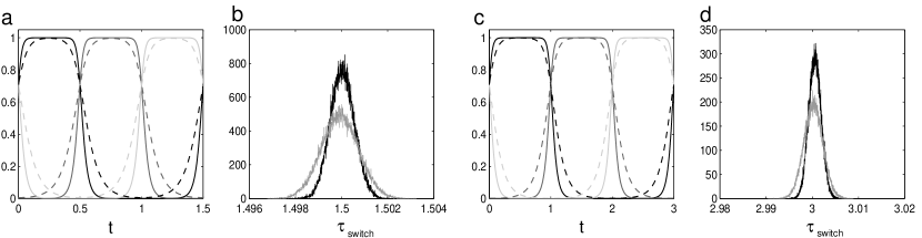
Figure 1: Stochastic Busse-Heikes model with parameters given in Table 1. (a) Evolution of the amplitudes: the solid lines correspond to (case a) in Table 1 and the dashed lines to (case b). (b) Period PDF for an integration time $t_{f}=1.5(10)^{5}$. The black curve (case a) has $\tau_{\text{switch}}=1.500$, standard deviation $\sigma=.0005$, skewness $\zeta=-.004$, and kurtosis $\kappa=-.022$. The gray curve (case b) has $\tau_{\text{switch}}=1.500$, $\sigma=.0008$, $\zeta=-.017$, and $\kappa=.057$. (c) Amplitudes for, (case e), solid lines, and (case f), dashed lines. (d) Period PDF for $t_{f}=3(10)^{5}$. For (case e), black, $\tau_{\text{switch}}=3.00$, $\sigma=.001$, $\zeta=.057$, and $\kappa=.002$, while for (case f), gray, $\tau_{\text{switch}}=3.000$, $\sigma=.003$, $\zeta=-.006$, and $\kappa=.018$.

Let $\tau_{\text{roll}}$ denote the typical scaled turnover time of a single roll (when $A=1$, $\tau_{\text{roll}}=\pi^{2}$, see Appendix A). The time $\tau_{\text{switch}}$ measures the effective strength of the rolls; consequently when

$$\frac{\tau_{\text{switch}}}{\tau_{\text{roll}}}<<1\;,$$ (14)

the strength of the rolls is relatively weak. As this parameter grows the rolls become stronger.

Let $\tau_{\text{trans}}$ denote the typical transition time between roll states (e.g., the transition time between $0^{\circ}$ and $120^{\circ}$ states). If the ratio of transition time to switching time is small:

$$\frac{\tau_{\text{trans}}}{\tau_{\text{switch}}}<<1\;,$$ (15)

then a relatively large time is spent in a particular roll state compared to the transition to the next roll. The parameter $\epsilon$ is the key to controlling this ratio; indeed, comparing the solid and dashed curves in in Fig. 1, it is clear that as $\epsilon$ grows this inequality becomes invalid.

5 Geometry

Since the vertical component of the velocity (1) vanishes at $z=\pm\pi/2$, the orbits are confined to the infinite domain

$$\mathcal{D}=\left\{(x,y,z):-\frac{\pi}{2}\leq z\leq\frac{\pi}{2}\right\}\;.$$ (16)

As we will review below, the velocity field (6) is invariant under a discrete translational symmetry generated by the unit vectors

$$\hat{u}_{1}=\left(1,0,0\right)\;,\quad\hat{u}_{2}=\left(\frac{1}{2},\frac{\sqrt{3}}{2},0\right)\;.$$

These vectors generate the planar “wallpaper” group denoted by $p3$:

$$p3=\left\{t_{mn}(\mathbf{x})=\mathbf{x}+\frac{4\pi}{\sqrt{3}}(m\hat{u}_{1}+n\hat{u}_{2}):m,n\in\mathbb{Z}\right\}\;.$$ (17)

corresponding to a single, order-three axis of symmetry. Here we have scaled the length of the vectors to correspond with the unit cell size in our examples. This group has a fundamental cell that is a regular hexagon, $\mathcal{H}$, of width $4\pi/\sqrt{3}$ and height $8\pi/3$, see Fig. 2.

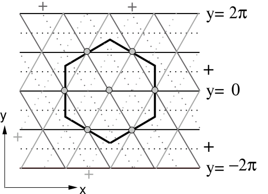
Figure 2: Schematic of the roll geometry in $z=0$ plane. The open circles correspond to saddle equilibria at $z=\pm\frac{\pi}{2}$. The solid lines correspond to roll boundaries and the dotted lines correspond to roll axes. The $+$ signs denote right-handed or positive rotation about its axis. The hexagon, $\mathcal{H}$ is a fundamental cell of the flow.

Regardless of the choice of time dependence for the amplitudes, the vector field (6) has a fourteen saddle equilibria on the upper and lower boundaries, $z=\pm\frac{\pi}{2}$; these are shown as the dots in Fig. 2. Each vertically separated pair is connected by an invariant line giving a heteroclinic connection. For example, the saddles at $\left(0,0,\pm\frac{\pi}{2}\right)$ are connected by the invariant line $\{x=y=0\}$. Along this heteroclinic connection, the fluid motion is downward. The remaining twelve saddles can be found on the boundary of $\mathcal{H}$, six at $z=\pi/2$ and six at $z=-\pi/2$. There are heteroclinic orbits connecting these pairs that move upward. For example, there is an upward moving heteroclinic connection between the points $\left(\frac{2\pi}{\sqrt{3}},0,-\frac{\pi}{2}\right)$ to $\left(\frac{2\pi}{\sqrt{3}},0,\frac{\pi}{2}\right)$.

Note that since the map (12) is an exact solution of (6) for the special case of step function amplitudes, the equilibria and heteroclinic connections of the flow become fixed points and heteroclinic lines of the map.

6 Numerical Explorations

In this section we study the mixing and transport for the flow (6) and compare it to that for the blinking roll mapping (12). One local measure of mixing corresponds to the Lyapunov exponents as a function of initial condition. There is a correlation between large exponents and regions of strong mixing. On the other hand in regions with many invariant tori, the exponents are zero or near zero.

A second measure is the rate of particle drift throughout the domain. A first goal is to distinguish between bounded and unbounded orbits. We will study those bounded orbits that remain within the fundamental domain $\mathcal{H}$—we call these orbits “trapped.” Generally the “regular” orbits appear to be trapped (for example, those on invariant tori), especially for the case $T_{1}=T_{2}=T_{3}$; however, there appear to be bounded invariant structures larger than a single fundamental domain when the mapping times are not equal. We will also compute the exit time distribution from a fundamental domain. Transport of unbounded orbits can be quantified by computing the growth rate of distance with $t$ and comparing this to diffusive behavior. Since the trajectories are bounded in $z$, we measure the drift in $(x,y)$ by looking at the growth rate of $r^{2}=x^{2}+y^{2}$.

6.1 Lyapunov Phase Portraits

In this section, we compute the three Lyapunov exponents, $(\mu_{1},\mu_{2},\mu_{3})$, as a function of initial condition for both the flow and map models. Ideally we would compute the exponents for each initial condition on a three-dimensional mesh covering the fundamental cell, but this would be prohibitively expensive in computation time and the results would be difficult to display. Instead, we use two, two-dimensional slices in the fundamental cell $\mathcal{H}$: the horizontal midplane, $z=0$, and the vertical cross section, $y=0$. The horizontal slice is hexagonal and is divided into a $70\times 70$ grid and the vertical slice is rectangular and divided into a $100\times 50$ grid.

Since the map is volume-preserving and the flow is incompressible, the sum $\mu_{1}+\mu_{2}+\mu_{3}=0$ for both models. In Fig. 3, we show only the value of the largest exponent $\mu_{1}$ for each initial condition on these grids. We call these pictures “Lyapunov phase portraits;” they help to differentiate between chaotic and regular regions and provide a local measure of chaos that correlates with rapid mixing. The exponents are computed using the QR method of Rangarajan et al [34, 35]. The second and third Lyapunov exponents were also computed for all cases. Typically we observed that $|\mu_{2}|\sim 10^{-4}$ which is two orders of magnitude smaller than $\mu_{1}$ in the chaotic region. Given that only $10^{5}$ iterations were used in the computation and that converge is slow, a longer integration might be expected to yield an evan smaller second exponent. Thus our results are consistent with $\mu_{2}=0$, and consequently with $\mu_{3}=-\mu_{1}$. Note that an autonomous flow always has a zero exponent. More generally, if the flow or map were reversible then we would also expect $\mu_{2}=0$. We have not been able to show, however, that our systems are reversible, and thus do not have an explanation for the near vanishing of $\mu_{2}$.

By computing the Lyapunov phase portraits for both the flow (6) and the map (12), a direct comparison can be made between the two dynamical systems if the parameter values are equivalent. For the flow we use a full integration of the stochastic Busse-Heikes model to generate the amplitude waveforms; those shown in Fig. 1 give a typical cycle. Since there are three blinking-rolls per map iteration, the corresponding parameter $T$ for the mapping is one third of the average period of the amplitude functions.

The results are shown in Fig. 3 and the corresponding parameter values are given in Table 1. In each case the total time corresponds to approximately $10^{5}$ oscillation cycles. The average period of oscillation is approximately $1.5$ for the first two flow cases (panels (a) and (b)), and we choose the corresponding mapping time in panel (c) to be $0.5$ so that the total integration time represented by iterating the map $10^{5}$ times is the same as that for the flow. For panels (e) and (f) the average period is $3.0$, and the corresponding mapping time $T=1.0$ is used in panel (g).

Results for the flow with $\eta=65^{\circ}$ are displayed in Fig. 3a and Fig. 3b. The amplitude waveforms in these two cases differ in their shapes, as shown by the solid and dashed curves in Fig. 1. The images indicate that there are toroidal regions of near zero Lyapunov exponent surrounded by a chaotic sea. The breaks in the toroidal region on the hexagonal slice correspond to locations where the torus does not intersect this slice. It is striking that the tori exist even when the three amplitude waveforms have significant intervals of overlap as they do for Fig. 3b. This suggests that the details of the amplitude wave form is not a critical factor in the existence of the tori. The corresponding Lyapunov phase portrait for the map, shown in Fig. 3c, is visually quite similar to (and as shown in Table 2 has a high correlation with) the first two flow cases. In Fig. 3e and Fig. 3f, the Lyapunov phase portraits are shown for the waveforms in Fig. 1c with $\eta=0^{\circ}$. Once again, these portraits show a high correlation with those for the corresponding mapping, shown in Fig. 3g. Although the $\eta=0^{\circ}$ case is nonphysical for rotating convection, it is interesting to see that the toroidal structures persist for small $\eta$ and are robust as this parameter varies.

Table 1: Parameters for the Lyapunov phase portraits of Fig. 3

Fig. 3	Model	$\eta$	$\alpha$	$\beta$	$\epsilon$	$\Delta t$	Period	$T$
a	flow	$65$	$29.9205$	$-27.9005$	$10^{-14}$	$.005$	$1.5$
b	flow	$65$	$12.7503$	$-10.7303$	$10^{-7}$	$.005$	$1.5$
c,d	map	$65$						$.5$
e	flow	$0$	$18.0225$	$-16.0025$	$10^{-16}$	$.01$	$3$
f	flow	$0$	$5.7560$	$-3.7360$	$10^{-8}$	$.01$	$3$
g,h	map	$0$						$1$

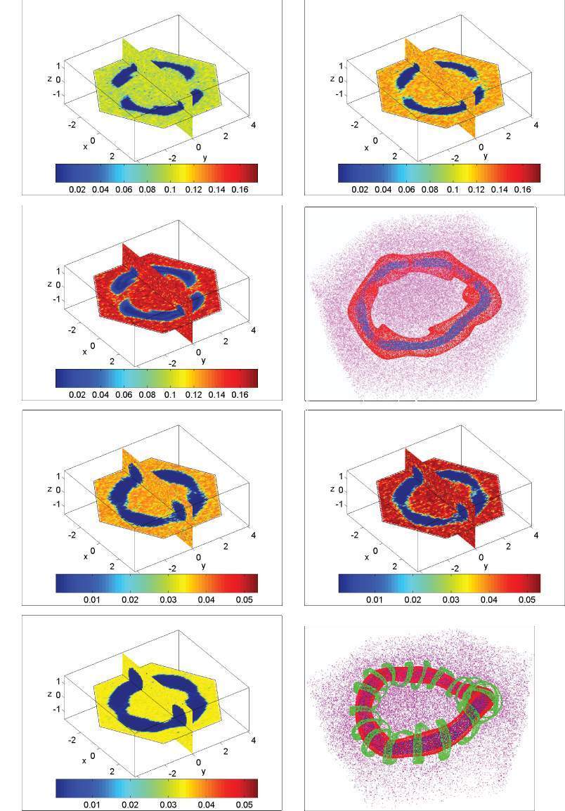
Figure 3: Lyapunov phase portraits for the flow (6) and map (12) for the parameter values given in Table 1. The largest Lyapunov exponent is computed by integrating or iterating for $10^{5}$ periods and the graphed values are obtained by averaging over the final $100$ periods. The color scale for $\mu_{1}$ is indicated at the bottom of each pane. Sample trajectories of the mapping are given in panels (d) and (h) showing regions occupied by invariant tori. Panels (a),(b), and (c) have the same color scale as do panels (e), (f), and (g).

A few orbits inside the regions of low chaos (red, blue, and green) and one in the chaotic region (purple) are shown in Fig. 3d for (12). The regions of near-zero Lyapunov exponent correspond to a set of nested two-dimensional tori. At the center of this nested set is apparently an elliptic, invariant curve. The green orbit in Fig. 3h appears to correspond to a torus that encloses an invariant curve that is helically wound about the central family of tori.

In each case, the close correlation between the Lyapunov exponents of the flow and mapping is clear from the pictures. To quantify this connection, we computed the correlation coefficient between the values of $\mu_{1}$ for mapping and for the flow on each slice. The results are given in Table 2; coefficients near one indicate similar structure whereas coefficients near zero suggest large differences between the data sets. In each case, a reasonably strong correlation is obtained. It is notable that as the ratio (15) increases, the correlation drops . This seems to predominantly occur near the outer boundary of the regular regions where the step function approximation to the amplitudes does a poor job of approximating the flow: the map tends to have a larger region foliated by invariant tori than does the flow.

Table 2: Correlation Coefficient of largest Lyapunov exponent between the map and the flow

Comparison	$\tau_{trans}/\tau_{switch}$	$y=0$ slice	$z=0$ slice
(a) vs. (c)	.19	.70	.88
(b) vs. (c)	.47	.69	.86
(e) vs. (g)	.16	.86	.94
(f) vs. (g)	.38	.74	.88

As computations with the map are much quicker than those for the flow it is easier to investigate the effect of changing parameters on the map. Moreover, changing the switching angle $\Theta$ from $120^{\circ}$ is problematic for the flow since the three-mode model (4) no longer applies. It is very easy, however, to change the switching angle in the map by choosing the rotation angle for the transformation $R$ in (12). One of the immediate observations is that tori are robust features of the mapping as the switching and tilt angles and time step $T$ are varied. For example, a large family of tori can be seen Fig. 4a (viewed from a camera looking down from large $z$). For this case the ratio (14) is small. The size of the innermost torus shown is on the order of one hexagonal convection cell; however, since $\Theta\neq 120^{\circ}$ the system no longer has hexagonal symmetry. Outside these tori, the motion is chaotic and diffusive (not shown in the figure).

A final example in Fig. 4b shows a number of helical tori enclosing the central family. In the center of the light gray orbits are invariant curves that wind twice in the toroidal direction before returning to their original positions. It is possible that these families of tori are created by period-doubling bifurcations of the invariant curve at the center of the main torus or a resonant bifurcation of a two-torus, but we have not verified this.

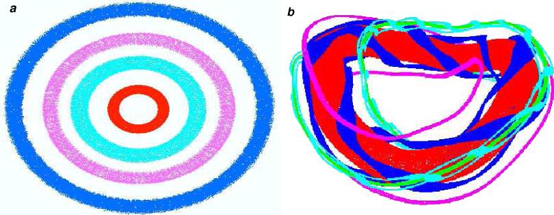
Figure 4: Phase portraits of (12) for (a) $T=.2$, $\eta=65^{\circ}$, and $\Theta=122^{\circ}$, and (b) $T=1$, $\eta=0^{\circ}$, $\Theta=45^{\circ}$. We plot points of the map $RF$ for each iterate instead of every third iterate as in (12).

There are too many parameters in the system to completely explore the full range of possible dynamics. A critical point is that the discrete symmetry does not produce the tori: these structures are features of the flow for many parameter values.

6.2 Breakdown of Integrability

When the time $T$ is very small, it is easy to see that the map (12) is, to first order in $T$, the same as the time-$T$ map of the autonomous field (7). Thus for a fixed total iteration time, we expect that the map dynamics will limit on the integrable flow of (7) as $T\rightarrow 0$. Indeed, we observe that the mapping shows the same closed, integrable trajectories of the classical hexagonal convection patterns [25] when $T$ approaches zero for a given fixed total time $nT$.

As $T$ grows, the closed trajectories are destroyed and are replaced by nested invariant tori separated by small zones of chaos as illustrated in Fig. 5. This example shows six families of “poloidal” two-tori linked with a central “toroidal” family. The poloidal tori can be seen crossing the $z=0$ section in the Lyapunov phase portrait of panel (a) near the center and edges of the hexagon. Invariant curves at the center of the poloidal and toroidal families of tori, shown in panel (b), can be found using the simple algorithm discussed in Appendix B. A trajectory in the chaotic region between the tori is shown in a top down view in panel (c). This domain can also be seen as the light grey regions in the Lyapunov phase portrait of panel (a).

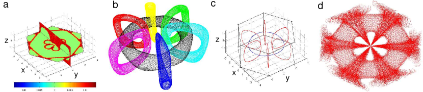
Figure 5: Phase portraits of (12) for $\Theta=120^{\circ}$, $\eta=0$, and $T=0.2$. Panel (a) shows the Lyapunov phase portrait, (b) the elliptic invariant curves at the center of the poloidal tori and (c) a chaotic trajectory in the region between the tori.

This same structure is seen when $T$ is small for any value of $\eta$. As $\eta$ increases the tori becomes increasingly twisted in the same manner as the classical hexagons. For each $\eta$, as $T$ is further increased, the six poloidal tori disappear leaving only the toroidal family. Eventually the toroidal family is destroyed as well and the cell appears to be completely chaotic (e.g. Fig. 6d below). In Table 3, the largest value of $T$ for which the map has visible tori is given as a function of $\eta$. For these $T$ values, the central invariant curves are warped and twisted (see Fig. 6a) and the surrounding two-tori have a small poloidal diameter. For large $\eta$, the transition from integrability to complete chaos is rapid.

Table 3: Largest time, $T$, for which (12) has invariant tori as $\eta$ varies

$\eta$	0	5	15	25	35	45	55	65	75	85
$T$	1.81	1.8	1.7	1.6	1.5	1.35	.97	.6	.6	.25

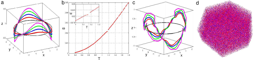
Figure 6: Toroidal invariant curves of (12) for $\eta=0$. (a) Curves for $T=0.2,0.6,1,1.4$, and $1.8$. The solid black line is (18). (b) Rotation Number $\omega$ as a function of mapping time $T$. (c) Phase portrait for $T=2$ where there are no invariant tori giving complete mixing.

The evolution of the toroidal invariant curve at the center of the toroidal family of two-tori is shown in more detail in Fig. 6. These curves are found using the center of mass algorithm algorithm of Appendix B. In panel (a), the curve is plotted for a number of different parameter values. As $T\rightarrow 0$ the invariant curve approaches the closed curve of the autonomous flow of (7) given by

$$\cos(y)+2\cos\left(\frac{\sqrt{3}x}{2}\right)\cos\left(\frac{y}{2}\right)=0\;.$$ (18)

This is shown as the darkest black curve at $z=0$. For larger $T$ values the invariant curve becomes increasingly distorted, and appears to lose differentiability. The curve is destroyed for $T\approx 1.81$. For larger values of $T$, as shown in panel (c), the phase portrait appears to be completely chaotic. Panel (b) shows the longitudinal rotation number of the invariant curves, $\omega$, as a function of $T$. As $T\rightarrow 0$, $\omega\rightarrow 0$ since the mapping limits to a time $T$ map of the autonomous flow. As $T$ increases the rotation number grows monotonically. There are gaps in the rotation number corresponding to parameter intervals where the curve is destroyed and reforms.

The six poloidal tori shown in Fig. 5 also appear to arise from streamlines of the autonomous, hexagonal flow (7) as $T$ increases from zero. Symmetry implies that they appear in the planes $x=0$ and $y=0$ and their rotations by $\pi/3$. When $\eta=0$, the streamlines of (7) in these planes correspond to contours of the functions

$$\Psi_{1}(0,y,z) = \cos(z)\sin^{2}\left(\frac{y}{2}\right)\left(\frac{1+2\cos(\frac{y}{2})}{1+\cos(\frac{y}{2})}\right)^{2}$$ (19)

$$\Psi_{2}(x,0,z) = \cos(z)\sin^{\frac{2}{3}}\left(\frac{\sqrt{3}x}{2}\right)\left(1-\cos\left(\frac{\sqrt{3}x}{2}\right)\right)^{\frac{2}{3}}\;,$$ (20)

respectively. When $\eta\neq 0$, a closed form expression for the streamlines is difficult to find. Using $T=10^{-4}$ and the center of mass algorithm, computations show that the invariant curves at the center of the six elliptic tori limit onto the streamline defined by $\Psi_{1}\approx 0.3868$ This streamline presumably is selected by a mechanism similar to the classical Poincaré-Birkhoff island chain created in when an integrable area-preserving map is perturbed.

Just as in the two-dimensional, island chain case, one of the $\Psi_{2}$ streamlines apparently becomes a hyperbolic (saddle) invariant curve in the same manner that the $\Psi_{1}=0.3868$ streamline becomes an elliptic invariant curve. Indeed, numerical computations show localized chaos around the planes $y=0$ and $y=\pm\sqrt{3}x$ (recall Fig. 5a and c) that grow as $T$ increases from zero. Transverse intersections of the stable and unstable manifolds of these saddle curves provide a mechanism for the onset of three-dimensional chaos [46].

The disappearance of the elliptic invariant curves as $T$ increases is expected to be caused by various resonant bifurcations between their longitudinal and transverse rotation numbers. This hypothesis is supported by the observation that the regular region surrounding the elliptic curves shrinks as they approach destruction. We hope to report further on these bifurcations in a future paper.

6.3 Transport

While Lyapunov exponents measure the divergence of neighboring trajectories, they give no information about how trajectories disperse over macroscopic distances, that is about “transport.” The goal of this section is to develop several measures of transport.

A first distinction to make is between trajectories that are bounded and those that are not. One class of bounded orbits are those that remain forever trapped in a single fundamental cell, $\mathcal{H}$. These, for example, include some of the invariant tori that we previously studied, though it is possible for invariant tori to exist on scales larger than a single cell. Since some trajectories never leave $\mathcal{H}$, it is reasonable to restrict the calculation to the set of initial conditions whose trajectories eventually do leave; this set is equivalent, up to a set of zero volume, to the subset that is “accessible” to trajectories that begin outside $\mathcal{H}$ [36]. The accessible set can be constructed by considering the incoming set $\mathcal{H}_{in}$ which is defined to be

$$\mathcal{H}_{in}=\mathcal{H}\setminus F(\mathcal{H})\;,$$

i.e., the portion of $\mathcal{H}$ that does not intersect $F(\mathcal{H})$. According to this definition, $F^{-1}(\mathcal{H}_{in})$ is outside of $\mathcal{H}$, thus every point in $\mathcal{H}_{in}$ has just entered $\mathcal{H}$. The accessible portion of $\mathcal{H}$ is the portion that can be reached by starting in the incoming set:

$$\mathcal{H}_{acc}=\bigcup\limits_{t=0}^{\infty}F^{t}(\mathcal{H}_{in})\cap\mathcal{H}\;.$$

In order to leave $\mathcal{H}$, a trajectory must first land in the exit set

$$\mathcal{H}_{exit}=\mathcal{H}\setminus F^{-1}(\mathcal{H})\;.$$

By volume preservation, the incoming and exit sets have the same volume.

A simple measure of transport is the “exit time distribution,” $\psi(t)$, defined to be the probability that a trajectory that starts in $\mathcal{H}_{in}$ at $t=0$, first leaves $\mathcal{H}$ at time $t$. To compute this we cover $\mathcal{H}$ with a grid of points. Each point is iterated with the inverse map to see if it remains in $\mathcal{H}$—if so, it is discarded. The remaining points are in the incoming set, and they are iterated forward until they exit $\mathcal{H}$.

Exit time distributions for hyperbolic systems are typically exponential; however, it is common in volume-preserving dynamics for $\psi$ to have a power-law form [21]:

$$\psi(t)\sim t^{-\gamma}\;.$$ (21)

For the case of a volume-preserving map, it is a consequence of Kac’s theorem that the average exit time

$$\tau_{exit}=\int_{0}^{\infty}t\psi(t)dt\;,$$ (22)

exists [36]. Thus $\psi(t)=o(t^{-2})$ as $t\rightarrow\infty$. The computations of exit time distributions, shown in Fig. 7a, are consistent with (21) and $\gamma\approx 2.1-2.5$. In each case, as the theory requires, $\tau_{exit}<\infty$ since the distribution has power law tail with $\gamma>2$.

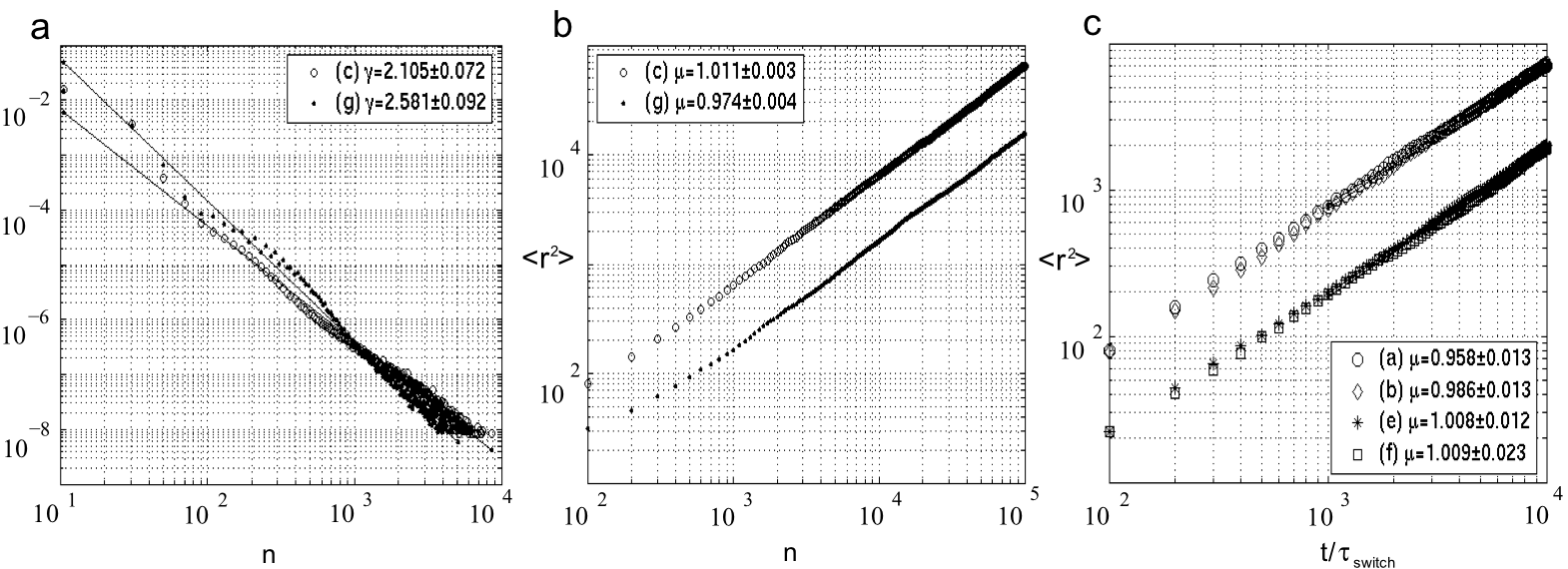
Figure 7: Exit time and mean square displacement with parameters given in Table 1 (a) Exit time distribution for a $1000\times 1000\times 500$ grid in fundamental cell. (b) Mean-squared displacement for $104$ randomly sampled points in $\mathcal{H}_{exit}$. (c) Mean-squared displacement for the flow (6) with amplitudes given in for $103$ randomly sampled points in $\mathcal{H}_{exit}$.

Chaotic trajectories that leave the fundamental cell tend to have unbounded orbits (though as we have seen there can also be superstructures extending over several copies of $\mathcal{H}$). One measure of the transport properties of unbounded trajectories is the growth rate of the mean-squared displacement, i.e.

$${\langle r^{2}(t)\rangle}\sim t^{\mu}\;.$$ (23)

The case $\mu=1$ corresponds to diffusive motion; however, many dynamical systems exhibit either subdiffusive ($\mu<1$) or superdiffusive ($\mu>1$) behavior [37]. Anomalous diffusion has been observed in many systems, for example, in two [39, 40] and three-dimensional fluids [7], plasma physics [38], and electron transport on semiconductor superlattices [41].

One phenomenological model that gives anomalous diffusion of the form of (23) is a continuous time random walk. In this model particles are assumed to move from one point to another under a sequence of “Lévy flights” whose length and duration are taken from probability distributions with power law tails. Such models display both normal and superdiffusive behavior [42, 43, 44]. A trapping probability distribution, separating jumps by trapping events in which the particle remains at its current position for a randomly selected time can also be added to the model—in our case this distribution is $\psi(t)$. For this situation, the dynamics can also exhibit subdiffusive behavior. Subdiffusion occurs when the motion is dominated by trapping events, and superdiffusion when flights are the more influential factor [45].

For our model the average exit time is finite; consequently, if there are no flights, one can expect normally diffusive behavior [47]. Though it is not easy to directly measure the distribution of particles undergoing so-called “Lévy flights,” we can compute the mean squared growth rate $\mu$, (23). To do this we randomly sample $10^{4}$ points in $\mathcal{H}_{exit}$, iterating each $10^{5}$ times. We also compute the mean square displacement for the continuous system, though in this case, since much computation is involve we only use $10^{3}$ initial points and integrate for $10^{4}$ periods. In both cases the results, shown in Fig. 7, are consistent with $\mu=1$ however $\mu=1$ does not always fall within the $90\%$ confidence interval. However, the least squares technique for computing the asymptotic growth rate may not give an accurate estimate of the error. In general though, it appears that these models are normally diffusive and that there are no Lévy flights, unlike many similar dynamical systems.

7 Discussion

We have studied two idealized, kinematic models of the Küppers-Lortz state. The building blocks of the models are vortical roll arrays whose axes are rotated through an angle $\Theta$ with respect to one another. In the continuous-time construction, the time dependence of the amplitude of the rolls is controlled by a stochastic Busse-Heikes system (4). When the amplitudes of the rolls are step functions and the rolls switch instantaneously from one set to another, we derived an analytical map, (12).

At the simplest level, the transition to chaos is governed by the the ratio of switching time, $\tau_{\mathrm{switch}}$, to turnover turnover time, $\tau_{\mathrm{roll}}$. As this parameter goes to zero, the flow approaches the autonomous, integrable case and when it is sufficiently small, the dynamics is similar, showing the classical hexagonal patterns observed in rotating Rayleigh-Bénard convection.

As this ratio grows, both the flow and the map have a family of invariant tori surrounding an elliptic invariant curve. Outside these tori is a chaotic sea. The tori undergo a complex sequence of bifurcations as the parameters change that we hope to report on in a future paper. In some cases we have also observed localized mixing for trajectories trapped within an invariant torus. This occurs, for example, if the central invariant curve is temporarily destroyed by a bifurcation, but the surrounding two-tori persist.

For large values of the the switching time, the Lyapunov phase portraits indicate nearly complete mixing. We characterized the transport properties of our system by computing the mean exit-time from the fundamental cell and the mean-squared drift of trajectories over the extended domain. Computations for the blinking-roll mapping and the flow showed algebraic decay of the exit time distribution, and the mean-squared growth consistent with normal diffusion. These results, in conjunction with anomalous diffusion theory, suggest that there is no analogue of the open streamlines in an autonomous flow or the “accelerator modes” of area-preserving maps that would effect long range, superdiffusive transport.

We also showed that the dynamics of the flow and map models is highly correlated even when the switching time is far from instantaneous. This observation suggests that a much broader class of continuous-time models, perhaps with periodic switching between more than three states, can be accurately modeled with the blinking roll mapping. With this in mind, one could easily extend the blinking roll system to include more realistic spatial descriptions for the flow, like Chandrasekhar functions, which are solutions to the linearized Boussinesq approximation with a no-slip lower boundary condition. However, it would be more difficult to obtain an explicit mapping and the computations would consequently be slower. For the simple case explored here, the Lyapunov phase portraits can be computed about twenty times faster for the map than for the flow.

The mapping has tori over a wide range of switching and tilt angles. We explored some of their behavior, but many mysteries remain. For instance, the middle Lyapunov exponent appears to be zero to numerical accuracy for both the continuous and discrete models. While this would be rigorously true for autonomous flows or reversible maps, we do not have an explanation of this for our systems. In addition, it would be interesting to study in detail the bifurcations that give rise to the families of invariant tori and curves, as well as those that ultimately lead to their destruction. Numerical studies show that destruction of invariant curves and tori typically enhances the mixing, but as of yet there is no satisfactory theory of transport for these three-dimensional systems.

Appendix A Appendix: Mean Roll Turnover Time

Here, we compute the average roll turnover time, $\tau_{\text{roll}}$, for a single roll with streamfunction $\psi=\sin(y)\cos(z)$. Suppose an initial condition is placed along the line $z=0$, $0<y=y_{0}<\frac{\pi}{2}$. The flow along this streamline is given by (9) (with $\eta=0$):

$$\Phi_{t}\left(x,y_{0},0\right)=\left(x,\text{sgn}(y_{0})\cos^{-1}\left(\frac{\cos(y_{0})\text{cn}(t)\text{dn}(t)}{1-\cos^{2}(y_{0})\text{sn}^{2}(t)}\right),\sin^{-1}\left(-\text{sn}(t)\cos(y_{0})\right)\right)\;.$$ (24)

Now, solve for the $t$ value such that

$$\Phi_{t}\left(x,y_{0},0\right)=\left(x,\frac{\pi}{2},y_{0}-\frac{\pi}{2}\right)\;.$$

This corresponds to one quarter of a rotation around a given streamfunction. This is possible since the tracers rotate counterclockwise in the domain $\left\{(x,y):0\leq y\leq\pi,-\frac{\pi}{2}\leq z\leq\frac{\pi}{2}\right\}$. From the third component, we find a simple equation for $t$:

$$t=\text{sn}^{-1}(1,k)=F\left(\frac{\pi}{2},k\right)\;.$$

Here, the modulus of the elliptic functions is (10) and $F(\frac{\pi}{2},k)$ is the complete elliptic integral of the first kind. To get the average roll turnover time for all streamfunctions, we integrate over $k$ to find [48]:

$$\tau_{\text{roll}}=4\int_{0}^{1}F\left(\frac{\pi}{2},k\right)dk=\pi^{2}\;.$$

It is straightforward to show that $\tau_{roll}$ is independent of $\eta$.

Appendix B Appendix: Finding Invariant Curves

Locating invariant curves is a more challenging task than finding fixed or periodic points of a map. For a map, the dynamics on an invariant curve is typically conjugate to a rigid rotation with irrational winding number. Therefore, one cannot use standard root finding techniques since the orbit never returns to itself. Though there are many standard algorithms for finding periodic orbits, methods for finding quasiperiodic ones are not as well developed. One algorithm uses Newton’s method coupled with an interpolation algorithm to find a single point on an invariant curve [49]. In another, the curve is approximated by a finite Forier series and Newton’s method is used to solve for the coefficients [50]. This this method is hindered by the assumption of conjugacy to rigid rotation number with an a priori known rotation number.

We use a simple algorithm that computes a single point on the invariant curve; however, only one point is needed since the rest of the invariant curve can be found through iteration. The method is limited because it only works for the case of an elliptic invariant curve, and it is rather slow. On the other hand, the method has significant advantages in that it does not require foreknowledge of the rotation number $\omega$ and it is easy to implement.

The first step is to choose an appropriate plane that is expected to intersect the invariant curve transversely. We fatten this plane into a thin slice of width $\epsilon$ and choose a point $\mathbf{x}_{0}$ in the slice close to where the curve is expected. Iterate the initial point and record the times it lands within the slice. Once $N$ such near returns are found, we compute the center of mass of these points, $\bar{\mathbf{x}}$. If the elliptic curve is surrounded by a family of two-tori, and these have a convex intersection with the slice then $\bar{\mathbf{x}}$ will approximate the position of the enclosed invariant curve. We now decrease $\epsilon$ and repeat the process with $\mathbf{x}_{0}=\bar{\mathbf{x}}$ as the new starting position. This procedure appears to work well to find a point on the invariant curve to machine precision. Given this point, we can now iterate to find the longitudinal rotation number $\omega$ of the curve.

References

- [1] J.M. Ottino. The Kinematics of Mixing: Stretching, Chaos, and Transport. Cambridge Univ. Press, Cambridge, 1989.
- [2] A.D. Stroock, S.K.W. Dertinger, A. Ajdari, I. Mezić, H.A. Stone, and G.M. Whitesides. Chaotic mixer for microchannels. Science, 295:647–651, 2002.
- [3] M.G. Brown and K.B. Smith. Ocean stirring and chaotic low-order dynamics. Physics of Fluids, 3:1186–1192, 1991.
- [4] C.K.R.T. Jones and S. Winkler. Invariant manifolds and Lagrangian dynamics in the ocean and atmosphere. Handbook of Dynamical Systems, Vol. 2, pages 55–92, 2002.
- [5] H. Aref. Stirring by chaotic advection. Journal of Fluid Mechanics, 143:1–21, 1984.
- [6] H. Aref. The development of chaotic advection. Physics of Fluids, 14:1315–1325, 2002.
- [7] M.A. Fogleman, M.J. Fawcett, and T.H. Solomon. Lagrangian chaos and correlated Lévy flights in a non-Beltrami flow: Transient versus long-term transport. Physical Review E, 63:1–4, 2001. 020101.
- [8] W.L. Vargas, L.E. Palacio, and D.M. Dominguez. Anomalous transport of particle tracers in multidimensional cellular flows. Physical Review E, 67:1–8, 2003. 026314.
- [9] P. Mullowney, K. Julien, and J.D. Meiss. Blinking rolls: Chaotic advection in a three-dimensional flow with an invariant. SIAM Journal on Applied Dynamical Systems, 4(1):159–186, 2005.
- [10] E. Moses and V. Steinberg. Stationary convection in a binary mixture. Physical Review A, 43(2):707–722, 1991.
- [11] G. Küppers and D. Lortz. Transition from laminar convection to thermal turbulence in a rotating fluid layer. Journal of Fluid Mechanics, 35(3):609–620, 1969.
- [12] G. Küppers. The stability of steady finite amplitude convection in a rotating fluid layer. Physics Letters A, 32:7–8, 1970.
- [13] Y. Hu, W. Pesch, G. Ahlers, and R.E. Ecke. Convection under rotation for Prandtl numbers near 1: Küppers-Lortz instability. Physical Review E, 58(5):5821–5833, 1998.
- [14] F. Zhong, R.E. Ecke, and V. Steinberg. Rotating Rayleigh-Bénard convection: Küppers-Lortz transition. Physica D, 51:596–607, 1991.
- [15] R.M. Clever and F.H. Busse. Nonlinear properties of convection rolls in a horizontal layers rotating about a vertical axis. Journal of Fluid Mechanics, 94:609–627, 1979.
- [16] T. Clune and E. Knobloch. Pattern selection in rotating convection with experimental boundary conditions. Physical Review E, 47(4):2536–2550, 1993.
- [17] L. Ning and R.E. Ecke. Küppers-Lortz transition at high dimensionless rotation rates in rotating Rayleigh-Bénard convection. Physical Review E, 47(5):R2991–R2994, 1993.
- [18] F.H. Busse and K.E. Heikes. Convection in a rotating layer - simple case of turbulence. Science, 208:173–175, 1980.
- [19] R. Toral, M. San Miguel, and R. Gallego. Period stabilization in the Busse-Heikes model of the Küppers-Lortz instability. Physica A, 280:315–336, 2000.
- [20] J. Klafter, M.F. Shlesinger, and G. Zumofen. Beyond Brownian motion. Physics Today, pages 33–39, February 1996.
- [21] J.D. Meiss. Symplectic maps, variational principles, and transport. Reviews of Modern Physics, 64(3):795–848, 1992.
- [22] G.O. Fountain, F.V. Khakhar, and J.M. Ottino. Visualization of three-dimensional chaos. Science, 281(31 July):683–686, 1998.
- [23] G. O. Fountain, D. V. Khakhar, I. Mezić, and J.M. Ottino. Chaotic mixing in a bounded three-dimensional flow. Journal of Fluid Mechanics, 417:265–301, 2000.
- [24] T. Shinbrot, M.M. Alvarez, J.M. Zalc, and F.J. Muzzio. Attraction of minute particles to invariant regions of volume preserving flows by transients. Physical Review Letters, 86(7):1207–1210, 2001.
- [25] S. Chandrasekhar. Hydrodynamic and Hydromagnetic Stability. Dover Publications, Inc., 1st edition, 1961.
- [26] K. Julien and E. Knobloch. Strongly nonlinear convection cells in a rapidly rotating fluid layer: the tilted f-plane. Journal of Fluid Mechanics, 360:141–178, 1998.
- [27] P. P. Niiler and F. E. Bisshopp. On the influence of Coriolis?force on onset of thermal convection. Journal of Fluid Mechanics, 22:753, 1965.
- [28] E. Stone and P. Holmes. Random perturbations of heteroclinic attractors. SIAM Journal on Applied Math, 50:726–743, 1990.
- [29] Y. Tu and M.C. Cross. Chaotic domain structure in rotating convection. Physical Review Letters, 69(17):2515–2518, 1992.
- [30] P.E. Kloeden and E. Platen. Numerical Solution of Stochastic Differential Equations. Springer-Verlag, Heidelberg, 1992.
- [31] K. Burrage and P.M. Burrage. High strong order explicit Runge-Kutta methods for stochastic ordinary differential equations. Applied Numerical Mathematics, 22:81–101, 1996.
- [32] J. W. S. Lamb and J. A. G. Roberts Time-Reversal Symmetry in Dynamical Systems: A Survey Phys. D 112: 1–39, 1998.
- [33] M. Field and M. Golubitsky. Symmetric chaos: How and why. Notices Amer. Math. Soc, 42(2):240–244, 1995.
- [34] S. Rangarajan, G.and Habib and R.D. Ryne. Lyapunov exponents without rescaling and reorthogonalization. Physical Review Letters, 80(17):3747–3750, 1998.
- [35] S. Habib, T.M. Janaki, G. Rangarajan, and R. D. Ryne. Computation of the Lyapunov spectrum for continuous-time dynamical systems and discrete maps. Physical Review E, 60(6):6614–6626, 1999.
- [36] J.D. Meiss. Average exit time for volume-preserving maps. Chaos, 7(1):139–147, 1997.
- [37] J. Klafter and R. Silbey. Derivation of the continuous-time random-walk equation. Physical Review Letters, 44(2):55–58, 1980.
- [38] D. del Castillo-Negrete, B.A. Carreras, and V.E. Lynch. Fractional diffusion in plasma turbulence. Physics of Plasmas, 11(9):3854–64, 2004.
- [39] T.H. Solomon, E.R. Weeks, and H.L. Swinney. Chaotic advection in a two-dimensional flow: Lévy flights and anomalous diffusion. Physica D, 76:70–84, 1994.
- [40] E.R. Weeks, J.S. Urbach, and H.L. Swinney. Anomalous diffusion in asymmetric random walks with a quasi-geostrophic flow example. Physica D, 97:291–310, 1996.
- [41] Fromhold, T.M. et.al. Chaotic electron diffusion through stochastic webs enhances current flow in superlattices. Nature, 428:726–730, 2004.
- [42] J. Klafter, A. Blumen, and M.F. Shlesinger. Stochastic pathway to anomalous diffusion. Physical Review A, 35(7):3081–3085, 1987.
- [43] G. Zumofen, J. Klafter, and A. Blumen. Anomalous transport: a one-dimensional stochastic model. Chemical Physics, 146:433–444, 1990.
- [44] J. Klafter, G. Zumofen, M.F. Shlesinger, and A. Blumen. Scale invariance in anomalous diffusion. Philosophical Magazine B, 65(4):755–765, 1992.
- [45] J. Klafter, G. Zumofen, and M.F. Shlesinger. Anomalous diffusion and Lévy statistics in intermittent chaotic systems. Lecture Notes in Physics, 457:183–210, 1995.
- [46] H.E. Lomelí, and J.D. Meiss. Heteroclinic intersections between invariant circles of volume-preserving maps. Nonlinearity, 16(5):1573–1595, 2003.
- [47] E.W. Montroll. Random walks on lattices. iii. calculation of first-passage times with application to exciton trapping on photosynthetic units. Journal of Mathematical Physics, 10(4):753–769, 1969.
- [48] P. F. Byrd and M. D. Friedman. Handbook of Elliptic Integrals for Engineers and Physicists. Springer Verlag, 1954.
- [49] E. Castella and Á. Jorba. On the vertical families of two-dimensional tori near the triangular points of the bicircular problem. Celestial Mechanics and Dynamical Astronomy, 76:35–54, 2000.
- [50] Á. Jorba. Numerical computation of the normal behavior of invariant curves of n-dimenional maps. Nonlinearity, 14(5):943–976, 2001.