A posteriori error control for discontinuous Galerkin methods for parabolic problems

A posteriori error control for discontinuous Galerkin methods for parabolic problems

Abstract.

We derive energy-norm a posteriori error bounds for an Euler time-stepping method combined with various spatial discontinuous Galerkin schemes for linear parabolic problems. For accessibility, we address first the spatially semidiscrete case, and then move to the fully discrete scheme by introducing the implicit Euler time-stepping. All results are presented in an abstract setting and then illustrated with particular applications. This enables the error bounds to hold for a variety of discontinuous Galerkin methods, provided that energy-norm a posteriori error bounds for the corresponding elliptic problem are available. To illustrate the method, we apply it to the interior penalty discontinuous Galerkin method, which requires the derivation of novel a posteriori error bounds. For the analysis of the time-dependent problems we use the elliptic reconstruction technique and we deal with the nonconforming part of the error by deriving appropriate computable a posteriori bounds for it. We illustrate the theory with a series of numerical experiments indicating the reliability and efficiency of the derived a posteriori estimates.

1. Introduction

Adaptive methods for partial differential equations (PDE’s) of evolution type have become a staple in improving the efficiency in large scale computations. Since the 1980’s many adaptive methods have been increasingly based on a posteriori error estimates, which provide a sound mathematical case for adaptive mesh refinement, which can be decomposed in spatially and temporally local error indicators. In the context of parabolic equations, a posteriori error estimates have been derived for various norms since early 1990’s [17, 36]. Inspired by the milestones set recently for the mathematical theory of convergence for adaptive methods in elliptic problems [33, 8, 13], there has been a recent push for similar results for parabolic problems calling to a closer understanding of a posteriori error estimates [15, 41, 7, 29, e.g.]. Most results in this area cover simple time-stepping schemes and a conforming space discretization. The extant literature on a posteriori error control for nonconforming spatial methods can be grouped in a handful of works [40, 18, 43, 34, 14]. In [40] a posteriori $\operatorname{L}_{2}(\operatorname{H}^{1})$-norm error bounds for a spatially semidiscrete method via interior penalty discontinuous Galerkin (IPDG) methods are derived and used heuristically in the implementation of the fully discrete scheme. In [18, 43] $\operatorname{L}_{2}(\operatorname{L}_{2})$-norm error bounds for IPDG are obtained using duality techniques, while in [34], a posteriori error bounds are presented for a fully discrete method consisting of a backward Euler time-stepping and linear Crouzeix–Raviart elements in space. Note that none of the papers in the literature, to our knowledge, cover the case of a posteriori energy-norm error bounds for fully discrete schemes with discontinuous Galerkin methods, which is the chief objective of our paper.

Discontinuous Galerkin (DG) methods are an important family of nonconforming finite element methods for elliptic, parabolic and hyperbolic problems dating back to 1970’s and early 1980’s [35, 37, 5, 42, 3]. DG methods have undergone substantial development in the recent years [16, 4, 39, 38, 24, e.g., and references therein]. The practical interest in DG methods owes to their flexibility in mesh design and adaptivity, in that they cover meshes with hanging nodes and/or locally varying polynomial degrees. DG methods are thus ideally suited for $hp$-adaptivity and provide good local conservation properties of the state variable. Moreover, in DG methods the local elemental bases can be chosen freely for the absence of interelement continuity requirements, yielding very sparse—in many cases even diagonal—mass matrices even with high precision quadrature. Note also that DG methods are popular due to their very good stability properties in transport- or convection-dominated problems [16]; the a posteriori error analysis of convection-dominated problems is, however, beyond the scope of our study and we concentrate on diffusion-only parabolic equations.

Our main results are a posteriori error bounds in the energy norm for a family of fully discrete approximations of the following PDE problem—in §2 we gather the functional analysis notation and background.

1.1 Problem (linear parabolic boundary-initial value problem).

Given an open (possibly curvilinear) polygonal domain $\varOmega\subseteq\mathbb{R}^{d}$, $d=2,3$, a real number $T>0$, two (generalized) functions

$$f\in\operatorname{L}_{\infty}(0,T;\operatorname{L}_{2}(\varOmega))\quad\text{and}\quad\boldsymbol{a}\in\operatorname{L}_{\infty}(\varOmega\times\left(0,T\right))^{d\times d},$$ (1.1)

such that $\boldsymbol{a}(x,t)$ is symmetric positive definite for almost all $(x,t)\in\varOmega\times\left[0,T\right]$, find a function $u\in\operatorname{L}_{2}(0,T;{\operatorname{H}^{1}_{0}(\varOmega)})$,

$$\partial_{t}{u}\in\operatorname{L}_{\infty}(0,T;\operatorname{H}^{-1}(\varOmega))$$ (1.2)

and such that

$$\begin{gathered}\partial_{t}{u}-\nabla\cdot(\boldsymbol{a}\nabla u)=f\text{ on }\varOmega\times\left(0,T\right],\\ u(0)=u_{0}\text{ on }\varOmega,\quad\text{and}\quad\left.u\right|_{\partial\varOmega}(t)=0,\text{ for }t\in\left(0,T\right].\end{gathered}$$ (1.3)

In §2 we propose a class of numerical methods for solving this problem. These methods consist in a backward Euler time-stepping scheme in combination with various choices of spatial DG methods. Our emphasis is on the widely applied IPDG method [3, 39, 24].

We consider the notation of Problem 1.1 to be valid throughout the paper and $u$ denotes the solution of problem (1.3). Although the assumption $f\in\operatorname{L}_{\infty}(0,T;\operatorname{L}_{2}(\varOmega))$ may be weakened—provided a posteriori error estimates for the corresponding spatial finite element method can be obtained for such weak data—we refrain from doing it for simplicity’s sake. In fact, we consider $f$ to be piecewise continuous in time with a finite number of time-discontinuities and with the implied constraints on the time partition, to be discussed in §2.4. The matrix-valued function $\boldsymbol{a}(\cdot,t)$, for each $t\in\left(0,T\right)$ is allowed to have jump discontinuities; the set of spatial discontinuities of $\boldsymbol{a}$ will be considered to be aligned with the finite element meshes. For simplicity, we shall assume that $\boldsymbol{a}$ is continuous in time, but a finite number of discontinuities can be accounted for easily, as long as these occur at the points of the time partition in the fully discrete scheme. The PDE (1.3) is assumed to be uniformly elliptic in the sense that the supremum and the infimum of the set

$$\left\{{\!\left({\boldsymbol{a}(x,t)\boldsymbol{\zeta}}\right)\cdot\boldsymbol{\zeta}}/{\left|\boldsymbol{\zeta}\right|^{2}}:\;\boldsymbol{\zeta}\in\mathbb{R}^{d},(x,t)\in\varOmega\times\left(0,T\right]\right\}$$ (1.4)

are both positive real numbers. As for the boundary values, we remark that our approach can be appropriately modified in order to extend homogeneous to general time-dependent Dirichlet boundary values. Under the assumptions made so far, we have that the solution to (1.3) exists and satisfies $u\in C(0,T;\operatorname{H}^{1}_{0}(\varOmega))$ and $\partial_{t}{u}\in\operatorname{L}_{2}(0,T;\operatorname{L}_{2}(\varOmega))$ [28].

In line with a unified approach to a posteriori error analysis for elliptic-problem DG methods [1, 2, 12] our discussion will be presented first in an abstract setting. Our results are then shown to be applicable to a wide class of DG methods provided that a posteriori error bounds for the corresponding steady-state problem are available.

We stress that, although we focus on a posteriori error bounds for spatial DG methods, our abstract results can be applied to a wider class of nonconforming methods (other than DG methods), provided they satisfy certain requirements. More specifically, given a particular nonconforming finite element space $S_{h}$, assume that:

• for each $Z\in S_{h}$ it is possible to decompose it as

  $$Z=Z_{c}+Z_{d}\text{ such that }Z_{c}\in{\operatorname{H}^{1}_{0}(\varOmega)}\cap S_{h},$$ (1.5)

  where $Z_{c}$ and $Z_{d}$ are called $Z$’s conforming part and the nonconforming part, respectively. This decomposition is an analytic device and is not needed for computational purposes. The only requirement on this decomposition is the ability to quantify certain norms of $Z_{d}$ in terms of $Z$, as found in the literature [6, 26, 23, e.g.], as well as our Lemma 4.3.

• Given a function $z\in{\operatorname{H}^{1}_{0}(\varOmega)}$, and let $Z\in S_{h}$ be the corresponding Ritz-projection via the finite element method, it is possible to bound the norm of the error $Z-z$, using a posteriori error estimators for the steady state problem.

A key tool in our a posteriori error analysis is the elliptic reconstruction technique [32]. Roughly speaking, the elliptic reconstruction technique, as far as energy estimates are concerned, allows to neatly separate the time discretization analysis form the spatial one. This technique, which has been adapted to tackle fully-discrete schemes via energy methods for conforming methods [29], is extended in this work to the nonconforming setting, to all methods that meet the two requirements above. Briefly said, the idea of elliptic reconstruction—denoting by $u$ the solution of (1.3) and by $U$ that of the discrete problem—consists in building an auxiliary function $w$, called the elliptic reconstruction of $U$, which satisfies two key properties: (a) a PDE-like relation binds the parabolic error $u-w$ with data quantities only involving $w-U$ and the problem’s data, $f$, $\boldsymbol{a}$, and $u_{0}$, (b) the function $U$ is the Ritz projection of $w$ onto $S_{h}$. Note that $w$ is an analysis-only device that, despite its name, it is not a computable object. Fortunately, computing $w$ is not needed in practice, as it does not appear in the resulting a posteriori bounds.

We believe that it is possible to obtain similar a posteriori error estimates, for each single method at hand, by working directly, i.e., without using an elliptic reconstruction technique, but this will inevitably lead to further complications which may render the analysis quite involved, especially for the fully discrete scheme. This prejudice of ours is testified by the somewhat surprising lack of previous rigorous results in the literature. Finally, we point out that it is possible to follow a similar approach to ours in order to derive a posteriori error estimates in lower order functional spaces such as $\operatorname{L}_{\infty}(0,T;\operatorname{L}_{2}(\varOmega))$.

We remark that new estimators arise in the derivation of fully discrete a posteriori error bounds, due to the time-dependent diffusion tensor considered in this work, compared to [29] where only time-independent diffusion coefficients are addressed.

The following is an outline of this article. After introducing the notation and the method in §2, the elliptic reconstruction is used to develop an abstract framework for spatially semidiscrete schemes in §3 and their fully discrete counterpart in §5. The actual error estimators for each particular method are then consequences of our abstract framework and specific elliptic error estimators such as the ones presented in [6, 26, 11, 23, 25, 19]. Moreover, in §4 we prove a posteriori bounds for the corresponding steady state problem of (1.1) for IPDG, thus extending existing results [6, 26, 23, 25] to the case of general (non-diagonal) diffusion tensor, with minimal regularity assumptions on the exact solution [19, cf.]. These a posteriori bounds are then combined with the general framework presented in in §3 and §5 to deduce fully computable bounds for the DG-approximation error of the parabolic problem. Last in §6 we summarize results from computer experiments aimed at exhibiting the reliability (derived theoretically) and efficiency of the error estimators in the special case of the IPDG method.

2. Preliminaries

2.1. Functional analysis tools

Given an open subset $\omega\subseteq\mathbb{R}^{d}$, we denote by $L^{p}(\omega)$, $1\leq p\leq\infty$, the Lebesgue spaces of functions with summable $p$-powers on $\omega$. The corresponding norms $\|\cdot\|_{L^{p}(\omega)}$; the norm of $\operatorname{L}_{2}(\omega)$ will be denoted by $\|{\cdot}\|_{\omega}$ for brevity; by $\langle\cdot,\cdot\rangle_{\omega}$ we write the standard $\operatorname{L}_{2}$-inner product on $\omega$. When $\omega=\varOmega$ we omit the subindex.

We denote by $\operatorname{H}^{s}(\omega)$, the standard Hilbert Sobolev space of index $s\in\mathbb{R}$; $\operatorname{H}^{1}_{0}(\omega)$ signifies the subspace of $\operatorname{H}^{1}(\omega)$ of functions with vanishing trace on the boundary $\partial\omega$. The Poincaré–Friedrichs inequality

$$\|{v}\|_{\varOmega}\leq C_{\operatorname{PF}}\|{\nabla v}\|_{\varOmega}\text{ for }v\in\operatorname{H}^{1}_{0}(\varOmega)$$ (2.1)

turns the $\operatorname{H}^{1}(\varOmega)$ seminorm into a norm on $\operatorname{H}^{1}_{0}(\varOmega)$. We consider thus $\|{\nabla\cdot}\|_{\varOmega}$ to be the norm on $\operatorname{H}^{1}_{0}(\varOmega)$. We will use also $\operatorname{H}^{-1}(\varOmega)$, the dual space of $\operatorname{H}^{1}_{0}(\varOmega)$, equipped with the duality brackets $\left\langle\cdot\,|\,\cdot\right\rangle$. Namely, if $f\in\operatorname{H}^{-1}(\varOmega)$ then for each $\phi\in\operatorname{H}^{1}_{0}(\varOmega)$ its value on $\phi$ is denoted by $\left\langle g\,|\,\phi\right\rangle$ which coincides with $\left\langle{g,\phi}\right\rangle$ if $g\in\operatorname{L}_{2}(\omega)$. Thus the norm of $g$ is given by

$$\left\|g\right\|_{\operatorname{H}^{-1}(\varOmega)}:=\sup_{\phi\in\operatorname{H}^{1}_{0}(\varOmega)\smallsetminus\left\{{0}\right\}}\frac{\left\langle{g,\phi}\right\rangle}{\left\|\nabla\phi\right\|}.$$ (2.2)

The duality pairing $\!\left({\operatorname{H}^{-1},\operatorname{H}^{1}_{0}}\right)$ allows us to define, for each fixed $t\in\left(0,T\right]$ the elliptic operator $\mathscr{A}(t):\operatorname{H}^{1}_{0}(\varOmega)\to\operatorname{H}^{-1}(\varOmega)$ where

$$\left\langle\mathscr{A}(t)v\,|\,\phi\right\rangle:=\left\langle{\boldsymbol{a}(t)\nabla v,\nabla\phi}\right\rangle\!\left({=\int_{\varOmega}\!\left({\boldsymbol{a}(x,t)\nabla v(x)}\right)\cdot{\nabla\phi(x)}\,\operatorname{d}\!x}\right)$$ (2.3)

$\text{ for }\phi,v\in\operatorname{H}^{1}_{0}(\varOmega)$. Here, and throughout the paper, we use the shorthand $f(t)=f(\cdot,t)$, for a function $f:[0,T]\times\varOmega\to\mathbb{R}$. Note that thanks to the uniform parabolic assumption given by (2.13) and the Lax–Milgram Theorem, the definition of the operator $\mathscr{A}(t)$ is well defined and yields an isomorphism between $\operatorname{H}^{-1}(\varOmega)$ and $\operatorname{H}^{1}_{0}(\varOmega)$ [21]. In other words, the operator $\mathscr{A}(t)$ induces a bounded coercive bilinear form

$$(v,w)\in\operatorname{H}^{1}_{0}(\varOmega)\times\operatorname{H}^{1}_{0}(\varOmega)\mapsto\left\langle\mathscr{A}(t)v\,|\,w\right\rangle\in\mathbb{R},$$ (2.4)

which we will extend later to a larger nonconforming space. We stress from the outset that although the bilinear form in (2.4) will be extended later to larger spaces, the operator $\mathscr{A}(t)$ will not and it will only act on $\operatorname{H}^{1}_{0}(\varOmega)$ functions throughout the discussion.

For $1\leq p\leq+\infty$, we also define the spaces $L^{p}(0,T,X)$, with $X$ being a real Banach space with norm $\|\cdot\|_{X}$, consisting of all measurable functions $v:[0,T]\to X$, for which

$$\begin{gathered}\|v\|_{L^{p}(0,T;X)}:=\Big{(}\int_{0}^{T}\|v(t)\|_{X}^{p}\mathrm{d}t\Big{)}^{1/p}<+\infty,\quad\text{for}\quad 1\leq p<+\infty,\\ \|v\|_{L^{\infty}(0,T;X)}:=\operatorname{ess\,sup}_{0\leq t\leq T}\|v(t)\|_{X}<+\infty,\quad\text{for}\quad p=+\infty.\end{gathered}$$ (2.5)

Finally, we denote by $C(0,T;X)$ the space of continuous functions $v:[0,T]\to X$ with norm $\|v\|_{C(0,T;X)}:=\max_{0\leq t\leq{T}}\|v(t)\|_{X}<+\infty$.

2.2. Finite element spaces

Let $\mathscr{T}$ be a subdivision of $\varOmega$ into disjoint open sets, which we call elements. We assume $\mathscr{T}$ to be parametrized by mappings $F_{\kappa}$, for each $\kappa\in\mathscr{T}$, where $F_{\kappa}:\hat{\kappa}\to\kappa$ is a diffeomorphism and $\hat{\kappa}$ is the reference element or reference square. The above mappings are such that $\bar{\varOmega}=\cup_{\kappa\in\mathscr{T}}\bar{\kappa}$. We often use the word mesh for subdivision, and we say that a mesh is regular if it has no hanging nodes; otherwise the mesh is irregular. Unless otherwise stated, we allow the mesh to be $1$-irregular, i.e., for $d=2$, there is at most one hanging node per edge, typically its center; for $d=3$ a corresponding concept is available.

For an integer $p\geq 1$, we denote by $\mathscr{P}_{p}(\hat{\kappa})$, the set of all polynomials on $\hat{\kappa}$ of degree $p$, if $\hat{\kappa}$ is the reference simplex, or of degree $p$ in each coordinate direction, if $\hat{\kappa}$ is the reference cube. We consider the discontinuous Galerkin finite element space

$$S=S^{p}(\mathscr{T}):=\{v\in\operatorname{L}_{2}(\varOmega):v_{\kappa}\circ F_{\kappa}\in\mathscr{P}_{p}(\hat{\kappa}),\,\kappa\in\mathscr{T}\}.$$ (2.6)

By $\varGamma$ we denote the union of all sides of the elements of the subdivision $\mathscr{T}$ (including the boundary sides). We think of $\varGamma$ as the union of two disjoint subsets $\varGamma=\varGamma_{\partial}\cup\varGamma_{\text{\rm int}}$, where $\varGamma_{\partial}$ is the union of all boundary sides.

Let two elements $\kappa^{+},\kappa^{-}\in\mathscr{T}$ have a common a side $e:=\bar{\kappa}^{+}\cap\bar{\kappa}^{-}\subset\varGamma_{\text{\rm int}}$. Define the outward normal unit vectors $\boldsymbol{n}^{+}$ and $\boldsymbol{n}^{-}$ on $e$ corresponding to $\partial\kappa^{+}$ and $\partial\kappa^{-}$, respectively. For functions $q:\varOmega\to\mathbb{R}$ and $\boldsymbol{\phi}:\varOmega\to\mathbb{R}^{d}$ uniformly continuous on each of $\kappa^{\pm}$, but possibly discontinuous across $e$, we define the following quantities. For $q^{+}:=q|_{\partial\kappa^{+}}$, $q^{-}:=q|_{\partial\kappa^{-}}$ and $\boldsymbol{\phi}^{+}:=\boldsymbol{\phi}|_{\partial\kappa^{+}}$, $\boldsymbol{\phi}^{-}:=\boldsymbol{\phi}|_{\partial\kappa^{-}}$, we set

$$\{\kern-4.55244pt\{q\}\kern-4.55244pt\}_{e} :=\frac{1}{2}(q^{+}+q^{-}),\quad \{\kern-4.55244pt\{\boldsymbol{\phi}\}\kern-4.55244pt\}_{e} :=\frac{1}{2}(\boldsymbol{\phi}^{+}+\boldsymbol{\phi}^{-}),$$ (2.7)

$$\left\llbracket q\right\rrbracket_{e} :=q^{+}\boldsymbol{n}^{+}+q^{-}\boldsymbol{n}^{-},\quad \left\llbracket\boldsymbol{\phi}\right\rrbracket_{e} :=\boldsymbol{\phi}^{+}\cdot\boldsymbol{n}^{+}+\boldsymbol{\phi}^{-}\cdot\boldsymbol{n}^{-};$$

if $e$ is a boundary side ($e\subset\varGamma_{\partial}$) these definitions are modified to

$$\{\kern-4.55244pt\{q\}\kern-4.55244pt\}_{e}:=q^{+},\ \{\kern-4.55244pt\{\boldsymbol{\phi}\}\kern-4.55244pt\}_{e}:=\boldsymbol{\phi}^{+},\ \left\llbracket q\right\rrbracket_{e}:=q^{+}\boldsymbol{n}^{+},\ \left\llbracket\boldsymbol{\phi}\right\rrbracket_{e}:=\boldsymbol{\phi}^{+}\cdot\boldsymbol{n}^{+}.$$ (2.8)

We introduce the mesh-size as the function $h:\varOmega\to\mathbb{R}$, by $h(x)=\operatorname{diam}\kappa$, if $x\in\kappa$ and $h(x)=\{\kern-4.55244pt\{h\}\kern-4.55244pt\}$, if $x\in\varGamma$. The shape-regularity of the subdivision $\mathscr{T}$ is defined as

$$\mu(\mathscr{T}):=\sup_{\kappa\in\mathscr{T}}\frac{h_{\kappa}}{r_{\kappa}},$$ (2.9)

where $r_{\kappa}$ is the radius of the largest ball that fits entirely in $\kappa$.

We shall use the gradient’s regular part operator, $\nabla_{\!\!\mathscr{T}}$, of an elementwise differentiable function $v$ defined by

$$(\nabla_{\!\!\mathscr{T}}v)|_{\kappa}:=\nabla(v|_{\kappa})\text{ for }\kappa\in\mathscr{T}.$$ (2.10)

Note that the full distributional gradient, $\nabla v$, consists of an extra term taking into account the jumps of $v$ across the edges (with a $-$ sign for historic reasons):

$$\nabla v=\nabla_{\!\!\mathscr{T}}v-\left\llbracket v\right\rrbracket\delta_{\varGamma_{\text{\rm int}}},$$ (2.11)

with $\delta_{\varGamma_{\text{\rm int}}}$ denoting the Dirac distribution on the interior skeleton $\varGamma_{\text{\rm int}}$. Finally, we consider some shorthand notation for quantities involving the diffusion tensor $a$. In particular, we define the elementwise constant functions $a_{\flat},a_{\sharp}:\varOmega\times[0,T]\to\mathbb{R}$ by

$$a_{\sharp}(\cdot,t)|_{\kappa}:=\||\sqrt{a}(\cdot,t)|_{2}\|_{L^{\infty}(\kappa)}^{2}\quad\text{and}\quad a_{\flat}(\cdot,t)|_{\kappa}:=\||(\sqrt{a}(\cdot,t))^{-1}|_{2}\|_{L^{\infty}(\kappa)}^{-2},$$ (2.12)

for $\kappa\in\mathscr{T}$, and $a_{\sharp}=\{\kern-4.55244pt\{a_{\sharp}\}\kern-4.55244pt\}$, $a_{\flat}=(\{\kern-4.55244pt\{1/a_{\flat}\}\kern-4.55244pt\})^{-1}$, on $\varGamma$, where $|\cdot|_{2}$ denotes the Euclidean-induced matrix norm. Finally, let

$$\alpha_{\sharp}(t):=\max_{x\in\varOmega}a_{\sharp}(x,t)\quad\text{and}\quad\alpha_{\flat}(t)=\min_{x\in\varOmega}a_{\flat}(x,t).$$ (2.13)

2.3. Spatial DG discretization

Introduce the DG space $\mathscr{S}:=S+\operatorname{H}^{1}_{0}(\varOmega)$, and a corresponding DG bilinear form $B:\mathscr{S}\times\mathscr{S}\to\mathbb{R}$, which we assume to be an extension of the bilinear form defined by (2.4), viz.,

$$B(t;v,z)=\left\langle\mathscr{A}(t)v\,|\,z\right\rangle\text{ for all }v,z\in\operatorname{H}^{1}_{0}(\varOmega),t\in\left(0,T\right].$$ (2.14)

Though $B$ is time-dependent, we do not write it explicitly in the semidiscrete case and omit the $t$.

The space $\mathscr{S}$ is equipped with a DG norm, denoted $|\kern-0.7113pt\|{\cdot}|\kern-0.7113pt\|$ and depending on the method at hand, which extends the energy norm, i.e.,

$$|\kern-0.7113pt\|{v}|\kern-0.7113pt\|=\|{\sqrt{a(\cdot,t)}\nabla v}\|\quad\text{for all}\ v\in\operatorname{H}^{1}_{0}(\varOmega),$$ (2.15)

for $t\in[0,T]$. Also here, the norm is time-dependent, but this dependence is not explicitly written. A norm equivalence between the energy norm $|\kern-0.7113pt\|{\cdot}|\kern-0.7113pt\|$ and $\|{\sqrt{a(\cdot,t)}\nabla\cdot}\|$ in $\operatorname{H}^{1}_{0}(\varOmega)$, uniformly with respect to $t$, suffices for all the bounds presented below to hold, modulo a multiplicative constant; but, we eschew this much generality for clarity’s sake.

The semidiscrete DG method in space for problem (1.3), reads as follows:

$$\begin{split}&\text{Find $U\in C^{0,1}(0,T;S_{h})$ such that}\\ &\langle\partial_{t}U,V\rangle+B(U,V)=\langle f,V\rangle\quad\text{ for }V\in S,t\in[0,T].\end{split}$$ (2.16)

We stress that these assumptions are satisfied by many DG methods for second order elliptic problems available in the literature, possibly by using inconsistent formulations [4]. Moreover, (2.14) and (2.15) are satisfied by IPDG (along with the corresponding energy norm) considered below as a paradigm.

Assumption (2.14) implies the consistency of the bilinear form $B$ on $\operatorname{H}^{1}_{0}(\varOmega)$, i.e.,

$$\langle\partial_{t}u,v\rangle+B(u,v)=\langle f,v\rangle,\quad\text{for all}\ v\in\operatorname{H}^{1}_{0}(\varOmega),$$ (2.17)

where $u$ is the exact (weak) solution to the initial-boundary value problem (1.3). Note that this is the same as writing

$$\partial_{t}{u}+\mathscr{A}u=f.$$ (2.18)

2.4. Fully discrete solution

To further discretize in time, consider an increasing time partition $\left\{{t_{n}}\right\}_{n=0,\dotsc,N}$, and the corresponding time-steps $\tau_{n}={t_{n}}-{t_{n-1}}$, for $n=1,\dotsc,N$. For each $n=0,\dotsc,N$, we consider that $S^{n}$ is a DG finite element space of fixed degree $p$ built on a partition $\mathscr{T}_{n}$, which may be different from $\mathscr{T}_{n-1}$ when $n\geq 1$. In §5.3, we will say more about the sequence of meshes and the compatibility relations among them.

Let $f^{n}(x):=f(x,{t_{n}})$ and let $U^{0}$ be the projection (or an interpolation) of $u_{0}$ onto the finite element space $S^{0}$. We say that $\left\{U^{n}\right\}_{n=0,\dotsc,N}$ is a fully discrete solution of (1.3) if, for each $n=1,\dotsc,N$ we have that $U^{n}\in S^{n}$ satisfies

$$\left\langle{(U^{n}-U^{n-1})/{\tau_{n}},V}\right\rangle+B^{n}\!\left({U^{n},V}\right)=\left\langle{f^{n},V}\right\rangle\quad\text{for all }V\in S^{n},$$ (2.19)

Since the elliptic operator $\mathscr{A}$ (and the bilinear form $B$) depend on time, in the fully discrete setting, we denote their value at time $t$ by $\mathscr{A}(t)$ and $B(t)$, respectively and when $t={t_{n}}$ we take $\mathscr{A}^{n}:=\mathscr{A}({t_{n}})$ and $B^{n}:=B({t_{n}})$.

Noting that the term $U^{n-1}$ can be replaced by $\varPi^{n}U^{n-1}$, where $\varPi^{n}:\operatorname{L}_{2}(\varOmega)\to S^{n}$ is the orthogonal projection, we consider a slightly more general situation where $\varPi^{n}U^{n-1}$ in (2.19) is replaced by $I^{n}U^{n-1}$; here $I^{n}:S^{n-1}\to S^{n}$ is a general data transfer operator, depending on the particular implementation. The operator $I^{n}$ may coincide with $\varPi^{n}$, but it may be an interpolation operator for example. The general fully discrete Euler scheme then reads

$$\left\langle{(U^{n}-I^{n}U^{n-1})/{\tau_{n}},V}\right\rangle+B^{n}\!\left({U^{n},V}\right)=\left\langle{f^{n},V}\right\rangle\quad\text{for all }V\in S^{n}.$$ (2.20)

We have taken $f^{n}=f({t_{n}})$, but we could take a more general approximation than $f({t_{n}})$, for example, a good choice is also given by $f^{n}:=\int_{t_{n-1}}^{t_{n}}f(s)\,\operatorname{d}\!s$, for which a suitable modification of our arguments leads to similar results.

3. Abstract a posteriori bounds for the semidiscrete problem

We derive next an abstract a posteriori error bound for the quantity

$$\|{u-U}\|_{\operatorname{L}_{2}(0,T;\mathscr{S})}:=\Big{(}\int_{0}^{T}|\kern-0.7113pt\|{u(t,\cdot)-U(t,\cdot)}|\kern-0.7113pt\|^{2}\Big{)}^{1/2},$$ (3.1)

where $|\kern-0.7113pt\|{\cdot}|\kern-0.7113pt\|$ denotes the appropriate (space) energy norm.

In the a posteriori error analysis below, we shall make use of the idea of elliptic reconstruction operators introduced in [32] for the semidiscrete problem and extended to fully discrete (conforming-in-space) methods in [29].

3.1 Definition (elliptic reconstruction and discrete operator).

Let $U$ be the (semidiscrete) DG solution to the problem (2.16). We define the elliptic reconstruction $w\in\operatorname{H}^{1}_{0}(\varOmega)$ of $U$ to be the solution of the elliptic problem

$$B(w,v)=\langle AU-\varPi f+f,v\rangle\quad\quad\text{for all }v\in\operatorname{H}^{1}_{0}(\varOmega),$$ (3.2)

where $\varPi:\operatorname{L}_{2}(\varOmega)\to S$ denotes the orthogonal $\operatorname{L}_{2}$-projection on the finite element space $S$, and $A:S\to S$ denotes the discrete DG operator defined by

$$\langle AZ,V\rangle=B(Z,V)\quad\text{for all }V\in S,$$ (3.3)

for each $Z\in S$. Note that this is valid on $\left[0,T\right]$.

3.2 Remark (the role of the elliptic reconstruction).

The elliptic reconstruction is well defined. Indeed, $AU\in S$ is the unique $\operatorname{L}_{2}$-Riesz representation of a linear functional on the finite dimensional space $S_{h}$ and the existence and uniqueness of (weak) solution of (3.2), with data $AU-\varPi f+f\in\operatorname{L}_{2}(\varOmega)$, follows from the Lax–Milgram Theorem in view of (2.14).

The key property of $w$ is that the DG solution $U$ of the semidiscrete time-dependent problem (2.16) is also the DG solution of the steady-state boundary-value problem (3.2). Indeed, let $W\in S$ be the DG-approximation to $w$, defined by the finite dimensional linear system

$$B(W,V)=\langle AU-\varPi f+f,V\rangle,$$ (3.4)

for all $V\in S$, which implies $B(W,V)=\langle AU,V\rangle=B(U,V)$ for all $V\in S$, i.e., $W=U$.

3.3 Definition (error, elliptic and parabolic parts).

We shall decompose the error as follows:

$$e:=U-u=\rho-\epsilon,\ \text{where}\ \epsilon:=w-U,\ \text{and}\ \rho:=w-u,$$ (3.5)

where $w=w(t)$ denotes the elliptic reconstruction of $U=U(t)$ at time $t\in[0,T]$. We call $\epsilon$ the elliptic error and $\rho$ the parabolic error.

3.4 Lemma (semidiscrete error relation).

Let $u$ be the solution of Problem 1.1, $U$ denote the solution of the DG scheme (2.16). Then, we have

$$\langle\partial_{t}e,v\rangle+B(\rho,v)=0\quad\text{for all }v\in\operatorname{H}^{1}_{0}(\varOmega).$$ (3.6)

Proof.

For each $v\in\operatorname{H}^{1}_{0}(\varOmega)$ we have

$$\langle\partial_{t}e,v\rangle+B(\rho,v)= \langle\partial_{t}U,v\rangle+B(w,v)-\langle f,v\rangle$$ (3.7)

$$= \langle\partial_{t}U,v\rangle+\langle AU-\varPi f+f,v\rangle-\langle f,v\rangle$$

$$= \langle\partial_{t}U,\varPi v\rangle+\langle AU,\varPi v\rangle-\langle f,\varPi v\rangle=0,$$

where in the first equality we used (2.17); in the second and fourth equalities, we made use of Definition 3.1; in the third equality the properties of the orthogonal $\operatorname{L}_{2}$-projection onto $S$ are used; finally, the last equality follows from (2.16).
$\Box$

3.5 Definition (conforming-nonconforming decomposition).

In the theory developed below, we shall consider the decomposition of the DG solution $U\in S$ into conforming (continuous) and nonconforming (discontinuous) parts as follows

$$U=U_{c}+U_{d},$$ (3.8)

where $U_{c}\in S_{c}:=\operatorname{H}^{1}_{0}(\varOmega)\cap S$ and $U_{d}:=U-U_{c}\in S$. Note that at this point we do not specify any particular decomposition, thus keeping the choice of such a decomposition at our disposal. Let

$$e_{c}:=e-U_{d}=U_{c}-u\in\operatorname{H}^{1}_{0}(\varOmega),\quad\text{and}\quad\epsilon_{c}:=\epsilon+U_{d}=w-U_{c}\in\operatorname{H}^{1}_{0}(\varOmega).$$ (3.9)

3.6 Theorem (long-time a posteriori error bound for DG).

Let $u$ and $U$ be the exact weak solution of (1.3) and the DG solution of the problem (2.16), respectively. Let $w$ be the elliptic reconstruction of $U$ as in Definition 3.1. Assuming (2.14) and (2.15), and that a decomposition of the form (3.8) is available, then the following error bound holds

$$\|{U-u}\|_{\operatorname{L}_{2}(0,T;\mathscr{S})}\leq 3\|{w-U}\|_{\operatorname{L}_{2}(0,T;\mathscr{S})}+2\|{U_{d}}\|_{\operatorname{L}_{2}(0,T;\mathscr{S})}$$ (3.10)

$$+2\|{\partial_{t}U_{d}/\sqrt{\alpha_{\flat}}}\|_{{\operatorname{L}_{2}(0,T;\operatorname{H}^{-1}(\varOmega))}}+2\|{u_{0}-U_{c}(0)}\|.$$

Proof.

Set $v=e_{c}$ in (3.6); then, in view of (3.9), we have

$$\langle\partial_{t}e_{c},e_{c}\rangle+B(\rho,\rho)=B(\rho,\epsilon_{c})-\langle\partial_{t}U_{d},e_{c}\rangle.$$ (3.11)

Recalling (2.14), (2.15) and that $\rho,e_{c}\in\operatorname{H}^{1}_{0}(\varOmega)$ for every $t\in[0,T]$, using the Cauchy–Schwarz inequality, and the duality pairing $\!\left({\operatorname{H}^{-1},\operatorname{H}^{1}_{0}}\right)$, we arrive to

$$\frac{1}{2}\mathrm{d}_{t}\|{e_{c}}\|^{2}+|\kern-0.7113pt\|{\rho}|\kern-0.7113pt\|^{2}\leq|\kern-0.7113pt\|{\rho}|\kern-0.7113pt\|\,|\kern-0.7113pt\|{\epsilon_{c}}|\kern-0.7113pt\|+\|{\partial_{t}U_{d}}\|_{\operatorname{H}^{-1}(\varOmega)}\|{\nabla e_{c}}\|.$$ (3.12)

Also, (3.9) implies

$$\|{e_{c}}\|_{\operatorname{H}^{1}(\varOmega)}\leq(|\kern-0.7113pt\|{\epsilon_{c}}|\kern-0.7113pt\|+|\kern-0.7113pt\|{\rho}|\kern-0.7113pt\|)/\sqrt{\alpha_{\flat}}.$$ (3.13)

Setting $I_{1}:=|\kern-0.7113pt\|{\epsilon_{c}}|\kern-0.7113pt\|$, $I_{2}:=\|{\partial_{t}{U_{d}}/\sqrt{\alpha_{\flat}}}\|_{\operatorname{H}^{-1}(\varOmega)}$ in (3.12) and rearranging lead to

$$\frac{1}{2}\mathrm{d}_{t}\|{e_{c}}\|^{2}+|\kern-0.7113pt\|{\rho}|\kern-0.7113pt\|^{2}\leq|\kern-0.7113pt\|{\rho}|\kern-0.7113pt\|(I_{1}+I_{2})+I_{1}I_{2},$$ (3.14)

which implies

$$\mathrm{d}_{t}\|{e_{c}}\|^{2}+|\kern-0.7113pt\|{\rho}|\kern-0.7113pt\|^{2}\leq 4(I_{1}^{2}+I_{2}^{2}).$$ (3.15)

Integration on $[0,T]$ and taking square roots yields

$$\|{\rho}\|_{\operatorname{L}_{2}(0,T;\mathscr{S})}\leq\|{e_{c}(0)}\|+2\|{\epsilon_{c}}\|_{\operatorname{L}_{2}(0,T;\mathscr{S})}+2\|{\partial_{t}U_{d}/\sqrt{\alpha_{\flat}}}\|_{{\operatorname{L}_{2}(0,T;\operatorname{H}^{-1}(\varOmega)})}.$$ (3.16)

The assertion follows using triangle inequality on (3.5) and (3.9).
$\Box$

3.7 Theorem (short-time a posteriori error bound for DG).

Let the assumptions of Theorem 3.6 hold. Then the following error bound holds:

$$\|{u-U}\|_{\operatorname{L}_{2}(0,T;\mathscr{S})}\leq (\sqrt{3/2}+1)\|{w-U}\|_{\operatorname{L}_{2}(0,T;\mathscr{S})}+\sqrt{3/2}\|{U_{d}}\|_{\operatorname{L}_{2}(0,T;\mathscr{S})}$$ (3.17)

$$+2\|{\partial_{t}U_{d}}\|_{L^{1}(0,T;\operatorname{L}_{2}(\varOmega))}+\sqrt{2}\|{u_{0}-U_{c}(0)}\|.$$

Proof.

Let $T_{0}\in[0,T]$ be such that

$$\|{e_{c}(T_{0})}\|=\max_{0\leq t\leq T}\|{e_{c}(t)}\|=:E_{c}.$$ (3.18)

Then, (3.11) implies

$$\frac{1}{2}\mathrm{d}_{t}\|{e_{c}}\|^{2}+|\kern-0.7113pt\|{\rho}|\kern-0.7113pt\|^{2}\leq|\kern-0.7113pt\|{\rho}|\kern-0.7113pt\|\,|\kern-0.7113pt\|{\epsilon_{c}}|\kern-0.7113pt\|+E_{c}\|{\partial_{t}U_{d}}\|,$$ (3.19)

which, after integration on $[0,T_{0}]$, yields

$$\frac{1}{2}E_{c}^{2}+\|{\rho}\|_{\operatorname{L}_{2}(0,T_{0};\mathscr{S})}^{2}\leq \frac{1}{2}\|{e_{c}(0)}\|^{2}+\|{\rho}\|_{\operatorname{L}_{2}(0,T_{0};\mathscr{S})}\|{\epsilon_{c}}\|_{\operatorname{L}_{2}(0,T_{0};\mathscr{S})}$$ (3.20)

$$+E_{c}\|{\partial_{t}U_{d}}\|_{L^{1}(0,T_{0};\operatorname{L}_{2}(\varOmega))},$$

or

$$\frac{1}{4}E_{c}^{2}\leq\frac{1}{2}\|{e_{c}(0)}\|^{2}+\frac{1}{4}\|{\epsilon_{c}}\|_{\operatorname{L}_{2}(0,T;\mathscr{S})}^{2}+\|{\partial_{t}U_{d}}\|_{L^{1}(0,T;\operatorname{L}_{2}(\varOmega))}^{2}.$$ (3.21)

Going back to (3.19), upon integration with respect to $t$ between $[0,T]$, we obtain

$$\frac{1}{2}\|{\rho}\|_{\operatorname{L}_{2}(0,T;\mathscr{S})}^{2}\leq\frac{1}{2}\|{e_{c}(0)}\|^{2}+\frac{1}{2}\|{\epsilon_{c}}\|_{\operatorname{L}_{2}(0,T;\mathscr{S})}^{2}+\frac{1}{4}E_{c}^{2}+\|{\partial_{t}U_{d}}\|_{L^{1}(0,T;\operatorname{L}_{2}(\varOmega))}^{2},$$ (3.22)

which, in conjunction with (3.21) gives

$$\|{\rho}\|_{\operatorname{L}_{2}(0,T;\mathscr{S})}^{2}\leq 2\|{e_{c}(0)}\|^{2}+\frac{3}{2}\|{\epsilon_{c}}\|_{\operatorname{L}_{2}(0,T;\mathscr{S})}^{2}+4\|{\partial_{t}U_{d}}\|_{L^{1}(0,T;\operatorname{L}_{2}(\varOmega))}^{2};$$ (3.23)

the final bound now follows using the triangle inequality on (3.5) and (3.9).
$\Box$

3.8 Remark (long- versus short-time bounds).

We note that the crucial difference between bounds (3.10) and (3.17) is that in the latter the $L^{1}$-accumulation term $\|{\partial_{t}U_{d}}\|_{L^{1}(0,T;\mathscr{S})}$ is present; this implies

$$\|{\partial_{t}U_{d}}\|_{L^{1}(0,T;\operatorname{L}_{2}(\varOmega))}\leq\sqrt{T}\|{\partial_{t}U_{d}}\|_{\operatorname{L}_{2}(0,T;\operatorname{L}_{2}(\varOmega))},$$ (3.24)

which may be preferable if $T<1$, but can be inefficient for long-time integration. On the other hand, the corresponding term in (3.10) is $\|{\partial_{t}{U_{d}}/\sqrt{\alpha_{\flat}}}\|_{{\operatorname{L}_{2}(0,T;\operatorname{H}^{-1}(\varOmega)})}$, which can be a bit less inefficient when the diffusion tensor $a$ varies substantially on $\varOmega$. We note, however, that it is possible to avoid dividing by the factor $\alpha_{\flat}$, by equipping $\operatorname{H}^{-1}(\varOmega)$ with the dual norm of the energy norm (2.15) in $\operatorname{H}^{1}_{0}(\varOmega)$. In practice, however, this improvement is relevant only if the dual norm is calculated explicitly [30]. Alternatively, one can apply a Poincaré–Friedrichs inequality to bound the dual norm by the $\operatorname{L}_{2}$-norm, which results into the reappearance of the factor $\alpha_{\flat}$.

3.9 Remark (elliptic a posteriori error estimates).

The bounds (3.10) and (3.17) are not (yet) explicitly a posteriori bounds: $\|{w-U}\|_{\operatorname{L}_{2}(0,T;\mathscr{S})}$ still needs to be bounded by a computable quantity. To this end, given $g\in\operatorname{L}_{2}$, consider the elliptic problem:

$$\begin{split}&\text{find $z\in\operatorname{H}^{1}_{0}(\varOmega)$ such that}\\ &-\nabla\cdot(\boldsymbol{a}\nabla z)=g\ \text{in }\varOmega,\quad z=0\text{ on }\partial\varOmega,\end{split}$$ (3.25)

whose solution can be approximated by the following DG method:

$$\begin{split}&\text{find $Z\in S$ such that}\\ &B(Z,V)=\langle g,V\rangle\quad\text{for all }V\in S.\end{split}$$ (3.26)

If assume that an a posteriori estimator functional $\mathscr{E}$ exists, i.e.,

$$|\kern-0.7113pt\|{z-Z}|\kern-0.7113pt\|\leq\mathscr{E}(Z,\boldsymbol{a},g,\mathscr{T}),$$ (3.27)

then we can computably bound $\|{w-U}\|_{\operatorname{L}_{2}(0,T;\mathscr{S})}$ in (3.10) and (3.17) through

$$\|{w-U}\|_{\operatorname{L}_{2}(0,T;\mathscr{S})}\leq\Big{(}\int_{0}^{T}\mathscr{E}(U,\boldsymbol{a},AU-\varPi f+f,\mathscr{T})^{2}\Big{)}^{1/2}.$$ (3.28)

A posteriori bounds for various DG methods have been studied, under different assumptions on data and admissible finite element spaces, by many authors [6, 26, 23, 2, 25, 19, 12]. Thus Theorems 3.6 and 3.7 can be applied to any DG—and more generally to any non-conforming—method satisfying (2.14) and (2.15), and for which (3.27) is available. The object of §4 is to address this for IPDG.

4. A posteriori error bounds for the interior penalty DG method

Here we extend the energy-norm a posteriori bounds for the family IPDG methods cf.[6, 26, 23] for the Poisson problem, to the case of the general diffusion problem (3.25). A similar analysis has recently appeared also in [19], while a related DG method based on weighted averages for anisotropic and high-contrast diffusion problems can be found in [20]. We stress that our results can be generalized as to allow for inhomogeneous or mixed boundary conditions following [23, 26, resp.].

4.1 Definition (IPDG method).

For $z,v\in\mathscr{S}$, the bilinear form $B:\mathscr{S}\times\mathscr{S}\to\mathbb{R}$ for the IPDG method for the problem (3.25) can be written as

$$B(z,v):=\int_{\varOmega}(\boldsymbol{a}\nabla_{\!\!\mathscr{T}}z)\cdot\nabla_{\!\!\mathscr{T}}v+\int_{\varGamma}\big{(}\theta\{\kern-4.55244pt\{\boldsymbol{a}\varPi\nabla v\}\kern-4.55244pt\}\cdot\left\llbracket z\right\rrbracket-\{\kern-4.55244pt\{\boldsymbol{a}\varPi\nabla z\}\kern-4.55244pt\}\cdot\left\llbracket v\right\rrbracket+\sigma\left\llbracket z\right\rrbracket\cdot\left\llbracket v\right\rrbracket\big{)},$$ (4.1)

for $\theta\in\{-1,0,1\}$, where $\varPi:[\operatorname{L}_{2}(\varOmega)]^{d}\to S^{d}$ denotes also the orthogonal $\operatorname{L}_{2}$-projection operator onto $S^{d}$, and the penalty function $\sigma:\varGamma\to\mathbb{R}$ is defined by

$$\sigma:=\frac{C_{\boldsymbol{a},\mu(\mathscr{T})}\{\kern-4.55244pt\{a_{\sharp}\}\kern-4.55244pt\}}{h},$$ (4.2)

where the constant $C_{\boldsymbol{a},\mu(\mathscr{T})}>0$ depends on the shape-regularity of the mesh $\mathscr{T}$ and on the smallest possible $C_{\boldsymbol{a}}>1$ such that

$$C_{\boldsymbol{a}}^{-1}\leq\frac{a_{\sharp}|_{\kappa^{+}}}{a_{\sharp}|_{\kappa^{-}}}\leq C_{\boldsymbol{a}},$$ (4.3)

for every pair of elements $\kappa^{+}$ and $\kappa^{-}$ sharing a common side.

We also define the corresponding energy norm $|\kern-0.7113pt\|{\cdot}|\kern-0.7113pt\|$ for the IPDG method by

$$|\kern-0.7113pt\|{v}|\kern-0.7113pt\|:=\Big{(}\|{\sqrt{\boldsymbol{a}}\nabla_{\!\!\mathscr{T}}v}\|^{2}+\|{\sqrt{\sigma}\left\llbracket v\right\rrbracket}\|_{\varGamma}^{2}\Big{)}^{1/2},$$ (4.4)

for $v\in\mathscr{S}$. Note that for $v\in S$, we have $\varPi\nabla v=\nabla v$ and, therefore, $B$ can be reduced to the more familiar form

$$B(z,v):=\int_{\varOmega}(\boldsymbol{a}\nabla_{\!\!\mathscr{T}}z)\cdot\nabla_{\!\!\mathscr{T}}v+\int_{\varGamma}\big{(}\theta\{\kern-4.55244pt\{\boldsymbol{a}\nabla v\}\kern-4.55244pt\}\cdot\left\llbracket z\right\rrbracket-\{\kern-4.55244pt\{\boldsymbol{a}\nabla z\}\kern-4.55244pt\}\cdot\left\llbracket v\right\rrbracket+\sigma\left\llbracket z\right\rrbracket\cdot\left\llbracket v\right\rrbracket\big{)},$$ (4.5)

for $z,v\in S$ [3, 4, 39, 24, cf.]. Observe that both (2.14) and (2.15) hold for the particular $B$ and $|\kern-0.7113pt\|{\cdot}|\kern-0.7113pt\|$ defined above.

4.2 Remark (conforming part of a nonconforming finite element function).

The space-discontinuous finite element space $S$ contains the conforming (continuous) finite element space $S_{c}=S\cap\operatorname{H}^{1}_{0}(\varOmega)$ as a subspace. The approximation of functions in $S$ by functions in $S_{c}$ will play an important role in our derivation of the a posteriori bounds. This can be quantified in the following result, which is an extension of [27, Thm. 2.1]. For other similar results we refer to [40, 6, 23, 10].

4.3 Lemma (bounding the nonconforming part via jumps).

Suppose $\mathscr{T}$ is a regular mesh and $\boldsymbol{a}$ is elementwise (weakly) differentiable. Then, for any function $Z\in S$ there exists a function $Z_{c}\in S_{c}$ such that

$$\|{Z-Z_{c}}\|\leq C_{1}\|{\sqrt{h}\left\llbracket Z\right\rrbracket}\|_{\varGamma},$$ (4.6)

and

$$\|{\sqrt{\boldsymbol{a}}\nabla_{\!\!\mathscr{T}}(Z-Z_{c})}\|\leq C_{2}\|{\sqrt{\sigma}\left\llbracket Z\right\rrbracket}\|_{\varGamma},$$ (4.7)

where $C_{1},C_{2}>0$ constants depending on the shape-regularity, on the maximum polynomial degree of the local basis and on $C_{\boldsymbol{a}}$.

The proof, omitted here, follows closely that of [26, Thm. 2.2]. Lemma 4.3 can be proved for irregular (i.e., with hanging-nodes) meshes [26, Thm. 2.3], in which case $C_{1}$ and $C_{2}$ depend on the maximum refinement and coarsening levels $L_{\max}$.

4.4 Lemma (a posteriori bounds for IPDG method for elliptic problem).

Let $\mathscr{T}$ be a regular and $\boldsymbol{a}$ is elementwise (weakly) differentiable. Let $z$ and $Z$ be given by (3.25) and (LABEL:dg_elliptic). Then

$$|\kern-0.7113pt\|{z-Z}|\kern-0.7113pt\|\leq\mathscr{E}_{\operatorname{IP}}(Z,\boldsymbol{a},g,\mathscr{T}),$$ (4.8)

where

$$\mathscr{E}_{\operatorname{IP}}(Z,\boldsymbol{a},g,\mathscr{T}):=CK_{\boldsymbol{a}}^{\mathscr{T}}\bigg{(} \|{h/\sqrt{a_{\flat}}(g+\nabla_{\!\!\mathscr{T}}\cdot(\boldsymbol{a}\nabla_{\!\!\mathscr{T}}Z))}\|$$ (4.9)

$$+\|{\sqrt{h/a_{\flat}}\left\llbracket\boldsymbol{a}\nabla_{\!\!\mathscr{T}}Z\right\rrbracket}\|_{\varGamma_{\text{\rm int}}}+\|{\sqrt{\sigma}\left\llbracket Z\right\rrbracket}\|_{\varGamma}\bigg{)},$$

and $K_{\boldsymbol{a}}^{\mathscr{T}}:=\max_{\varOmega}\sqrt{a_{\sharp}/a_{\flat}}$, where $C>0$ depends only on $\mu(\mathscr{T})$ and $C_{\boldsymbol{a}}$.

Proof.

Our proof is inspired by [26, 23]. Denoting by $Z_{c}\in S_{c}$ the conforming part of $W$ as in Lemma 4.3, we have

$$e:=z-Z=e_{c}+e_{d},\quad\text{where}\quad e_{c}:=z-Z_{c},\quad\text{and}\quad e_{d}:=Z_{c}-Z,$$ (4.10)

yielding $e_{c}\in\operatorname{H}^{1}_{0}(\varOmega)$. Thus, we have $B(z,e_{c})=\langle g,e_{c}\rangle$. Let $\varPi_{0}:\operatorname{L}_{2}(\varOmega)\to\mathbb{R}$ denote the orthogonal $\operatorname{L}_{2}$-projection onto the elementwise constant functions; then $\varPi_{0}e_{c}\in S$ and we define $\eta:=e_{c}-\varPi_{0}e_{c}$.

We also have

$$B(e,e_{c})=B(z,e_{c})-B(Z,e_{c})=\langle g,e_{c}\rangle-B(Z,\eta)-B(Z,\varPi_{0}e_{c})=\langle g,\eta\rangle-B(Z,\eta),$$ (4.11)

which implies

$$\|{\sqrt{a}\nabla e_{c}}\|^{2}=B(e_{c},e_{c})=\langle g,\eta\rangle-B(Z,\eta)-B(e_{d},e_{c}).$$ (4.12)

For the last term on the right-hand side of (4.12), we have

$$|B(e_{d},e_{c})|\leq\|{\sqrt{\boldsymbol{a}}\nabla_{\!\!\mathscr{T}}e_{d}}\|\|{\sqrt{\boldsymbol{a}}\nabla e_{c}}\|+\frac{1}{2}\sum_{s\subset\varGamma}\sum_{\kappa=\kappa^{+},\kappa^{-}}a_{\sharp}|_{\kappa}\|{\sqrt{h}(\varPi\nabla e_{c})|_{\kappa}}\|_{e}\|{\left\llbracket e_{d}\right\rrbracket/\sqrt{h}}\|_{s},$$ (4.13)

where $\kappa^{+}$ and $\kappa^{-}$ are the (generic) elements having $e$ as common side. Using the inverse estimate of the form $\|{\sqrt{h}V}\|_{e}\leq C\|{V}\|_{\kappa}$ for $V=\varPi\nabla e_{c}$, and the stability of the $\operatorname{L}_{2}$-projection, we arrive to

$$|B(e_{d},e_{c})|\leq\|{\sqrt{\boldsymbol{a}}\nabla_{\!\!\mathscr{T}}e_{d}}\|\|{\sqrt{\boldsymbol{a}}\nabla e_{c}}\|+CK_{\boldsymbol{a}}^{\mathscr{T}}\|{\sqrt{\boldsymbol{a}}\nabla e_{c}}\|\|{\sqrt{\sigma}\left\llbracket e_{d}\right\rrbracket}\|_{\varGamma}.$$ (4.14)

Finally, noting that $\left\llbracket e_{d}\right\rrbracket=\left\llbracket Z\right\rrbracket$, and making use of (4.7) we conclude that

$$|B(e_{d},e_{c})|\leq CK_{\boldsymbol{a}}^{\mathscr{T}}\|{\sqrt{\boldsymbol{a}}\nabla e_{c}}\|\,\|{\sqrt{\sigma}\left\llbracket W\right\rrbracket}\|_{\varGamma}.$$ (4.15)

To bound the first two terms on the right-hand side of (4.12), we begin by an elementwise integration by parts yielding

$$\langle g,\eta\rangle-B(Z,\eta)= \int_{\varOmega}\big{(}g+\nabla_{\!\!\mathscr{T}}\cdot(\boldsymbol{a}\nabla_{\!\!\mathscr{T}}Z)\big{)}\eta-\int_{\varGamma_{\text{\rm int}}}\{\kern-4.55244pt\{\eta\}\kern-4.55244pt\}\left\llbracket\boldsymbol{a}\nabla Z\right\rrbracket\mathrm{d}s$$ (4.16)

$$+\int_{\varGamma}\theta\{\kern-4.55244pt\{\boldsymbol{a}\varPi\nabla\eta\}\kern-4.55244pt\}\cdot\left\llbracket Z\right\rrbracket\mathrm{d}s-\int_{\varGamma}\sigma\left\llbracket Z\right\rrbracket\cdot\left\llbracket\eta\right\rrbracket\mathrm{d}s.$$

The first term on the right-hand side of (4.16) can be bounded as follows:

$$\Big{|}\int_{\varOmega}\big{(}g+\nabla\cdot(\boldsymbol{a}\nabla Z)\big{)}\,\eta\,\Big{|}\leq\|{h/\sqrt{a_{\flat}}(g+\nabla_{\!\!\mathscr{T}}\cdot(\boldsymbol{a}\nabla_{\!\!\mathscr{T}}Z))}\|\|{\sqrt{a_{\flat}}h^{-1}\eta}\|;$$ (4.17)

upon observing that $\|{h^{-1}\eta}\|_{\kappa}\leq C\|{\nabla e_{c}}\|_{\kappa}$, this becomes

$$\Big{|}\int_{\varOmega}\big{(}g+\nabla\cdot(\boldsymbol{a}\nabla Z)\big{)}\,\eta\Big{|}\leq CK_{\boldsymbol{a}}^{\mathscr{T}}\|{h/\sqrt{a_{\flat}}(g+\nabla_{\!\!\mathscr{T}}\cdot(\boldsymbol{a}\nabla_{\!\!\mathscr{T}}Z))}\|\|{\sqrt{\boldsymbol{a}}\nabla e_{c}}\|.$$ (4.18)

For the second term on the right-hand side of (4.16), we use a trace estimate, the bound $\|{h^{-1}\eta}\|_{\kappa}\leq C\|{\nabla e_{c}}\|_{\kappa}$ and we observe that $\nabla\eta=\nabla e_{c}$, to deduce

$$\Big{|}\int_{\varGamma_{\text{\rm int}}}\{\kern-4.55244pt\{\eta\}\kern-4.55244pt\}\left\llbracket\boldsymbol{a}\nabla Z\right\rrbracket\mathrm{d}s\Big{|}\leq CK_{\boldsymbol{a}}^{\mathscr{T}}\|{\sqrt{\boldsymbol{a}}\nabla e_{c}}\|\,\|{\sqrt{h/a_{\flat}}\left\llbracket\boldsymbol{a}\nabla_{\!\!\mathscr{T}}Z\right\rrbracket}\|_{\varGamma_{\text{\rm int}}}.$$ (4.19)

For the third term on the right-hand side of (4.16), we use $\nabla\eta=\nabla e_{c}$ and, working alike to (4.13), we obtain

$$\Big{|}\int_{\varGamma}\theta\{\kern-4.55244pt\{\boldsymbol{a}\varPi\nabla\eta\}\kern-4.55244pt\}\cdot\left\llbracket Z\right\rrbracket\Big{|}\leq CK_{\boldsymbol{a}}^{\mathscr{T}}|\theta|\|{\sqrt{\boldsymbol{a}}\nabla e_{c}}\|\,\|{\sqrt{\sigma}\left\llbracket Z\right\rrbracket}\|_{\varGamma},$$ (4.20)

and finally, for the last term on the right-hand side of (4.16), we get

$$\Big{|}\int_{\varGamma}\sigma\left\llbracket\eta\right\rrbracket\cdot\left\llbracket Z\right\rrbracket\Big{|}\leq CK_{\boldsymbol{a}}^{\mathscr{T}}\|{\sqrt{\boldsymbol{a}}\nabla e_{c}}\|\,\|{\sqrt{\sigma}\left\llbracket Z\right\rrbracket}\|_{\varGamma}.$$ (4.21)

The result follows combining the above relations.
$\Box$

4.5 Theorem (a posteriori bounds for IPDG method for parabolic problem).

Let $u,U$ be the exact weak solution of (1.3), and the IPDG solution of the problem (2.16), respectively, and let $\boldsymbol{a}$ be elementwise (weakly) differentiable. Then, the following error bound holds:

$$\|{u-U}\|_{\operatorname{L}_{2}(0,T;\mathscr{S})}^{2}\leq C\int_{0}^{T}\big{(}\mathscr{E}_{\operatorname{IP}}^{2}(U,\boldsymbol{a},AU-\varPi f+f,\mathscr{T})+\alpha_{\flat}^{-1}\|{\sqrt{h}\left\llbracket\partial_{t}U\right\rrbracket}\|_{\varGamma}^{2}\big{)}$$ (4.22)

$$+C\big{(}\|{u_{0}-U(0)}\|+\|{\sqrt{h}\left\llbracket U(0)\right\rrbracket}\|\big{)}^{2}.$$

If we assume also that $u,U\in C(0,T;\operatorname{H}^{1}_{0}(\varOmega))\cap\operatorname{H}^{1}(0,T;\operatorname{L}_{2}(\varOmega))$, then the following bound also holds:

$$\|{u-U}\|_{\operatorname{L}_{2}(0,T;\mathscr{S})}^{2}\leq C\int_{0}^{T}\mathscr{E}_{\operatorname{IP}}^{2}(U,\boldsymbol{a},AU-\varPi f+f,\mathscr{T})+C\Big{(}\int_{0}^{T}\|{\sqrt{h}\left\llbracket\partial_{t}U\right\rrbracket}\|_{\varGamma}\Big{)}^{2}$$ (4.23)

$$+C\big{(}\|{u_{0}-U(0)}\|+\|{\sqrt{h}\left\llbracket U(0)\right\rrbracket}\|\big{)}^{2}.$$

Proof.

The results follow immediately from combining Theorems 3.6 and 3.7 with Lemma 4.4, in conjunction with (4.6).
$\Box$

Finally, we give a result on useful properties of the IPDG bilinear form and of the norm, which will be useful in §5.

4.6 Lemma (continuity of $B$ and stability of the $\operatorname{L}_{2}$-projection).

Consider the notation of §4 and let $B$ and $|\kern-0.7113pt\|{\cdot}|\kern-0.7113pt\|$ denote the IPDG bilinear form (4.5) and the DG-norm (4.4). Then for $Z,V\in S_{h}$ we have

$$B(Z,V)\leq CK_{\boldsymbol{a}}^{\mathscr{T}}|\kern-0.7113pt\|{Z}|\kern-0.7113pt\||\kern-0.7113pt\|{V}|\kern-0.7113pt\|.$$ (4.24)

Moreover, for $v\in\operatorname{H}^{1}_{0}(\varOmega)$, the $\operatorname{L}_{2}$-projection is DG-norm-stable, i.e.,

$$|\kern-0.7113pt\|{\varPi v}|\kern-0.7113pt\|\leq CK_{\boldsymbol{a}}^{\mathscr{T}}|\kern-0.7113pt\|{v}|\kern-0.7113pt\|.$$ (4.25)

Proof.

We omit the proof of (4.24) which mimics that of (4.15). For stability, note

$$|\kern-0.7113pt\|{\varPi v}|\kern-0.7113pt\|^{2}= \|{\sqrt{\boldsymbol{a}}\nabla_{\!\!\mathscr{T}}(\varPi v-\varPi_{0}v)}\|^{2}+\|{\sqrt{\sigma}\left\llbracket v-\varPi v\right\rrbracket}\|_{\varGamma}^{2}$$ (4.26)

$$\leq C\Big{(}\|{a_{\sharp}^{\frac{1}{2}}h^{-1}(\varPi v-\varPi_{0}v)}\|^{2}+\|{a_{\sharp}^{\frac{1}{2}}h^{-1}(v-\varPi v)}\|^{2}+\|{a_{\sharp}^{\frac{1}{2}}\nabla_{\!\!\mathscr{T}}(v-\varPi v)}\|^{2}\Big{)}$$

$$\leq C\Big{(}\|{a_{\sharp}^{\frac{1}{2}}h^{-1}(v-\varPi_{0}v)}\|^{2}+\|{a_{\sharp}^{\frac{1}{2}}\nabla_{\!\!\mathscr{T}}(v-\varPi v)}\|^{2}\Big{)}$$

$$\leq C\|{(a_{\sharp}/a_{\flat})^{\frac{1}{2}}\sqrt{\boldsymbol{a}}\nabla_{\mathscr{T}}v}\|^{2},$$

which implies (4.25).
$\Box$

5. A posteriori error bound for the fully discrete scheme

In this section we discuss the abstract error analysis for the fully discrete scheme defined in §2.4.

5.1. The elliptic reconstruction and the basic error relation

Extend the sequence $\left\{U^{n}\right\}$ into a continuous piecewise linear function of time:

$$U(0)=U^{0}\quad\text{and}\quad U(t)=l_{n}(t)U^{n}+l_{n-1}(t)U^{n-1},$$ (5.1)

for $t\in\left[{t_{n-1}},{t_{n}}\right]$, and $n=1,\dotsc,N$, where the functions $l_{n}$ and $l_{n-1}$ are the Lagrange basis functions

$$l_{n}(t):=\frac{t-{t_{n-1}}}{\tau_{n}}\mathbb{1}_{\left[{t_{n-1}},{t_{n}}\right]}+\frac{t_{n+1}-t}{\tau_{n+1}}\mathbb{1}_{\left[{t_{n}},t_{n+1}\right]}.$$ (5.2)

Using these time extensions and the (time and mesh dependent) discrete elliptic operator $A^{n}$ of Definition 3.1 with respect to $S^{n}$, defined by

$$A^{n}Z\in S^{n}\text{ such that }\left\langle{A^{n}Z,V}\right\rangle=B^{n}\!\left({Z,V}\right)\quad\text{for all }V\in S^{n},$$ (5.3)

we can write the scheme (2.20) in the following pointwise form:

$$\partial_{t}{U}(t)+A^{n}U^{n}=(I^{n}U^{n-1}-U^{n-1})/\tau_{n}+\varPi^{n}f^{n},$$ (5.4)

for all $t\in\left({t_{n-1}},{t_{n}}\right),n=1,\dotsc,N$.

We like to warn at this point that we use the same symbol $U(t)$ to indicate the fully discrete solution time-extension in this section, and the semidiscrete solution in §3. This should cause no confusion as long as the two cases are kept in separate sections.

For each fixed $t\in\left[0,T\right]$, and the corresponding $n=1,\dotsc,N$ such that $t\in\left({t_{n-1}},{t_{n}}\right]$, we define the time-dependent elliptic reconstruction to be the function $w(t)\in{\operatorname{H}^{1}_{0}(\varOmega)}$ satisfying

$$w(t)=l_{n}(t)w^{n}+l_{n-1}(t)w^{n-1}_{+},$$ (5.5)

where $w^{n}\in{\operatorname{H}^{1}_{0}(\varOmega)}$ is the elliptic reconstruction of $U^{n}$ defined implicitly as the (weak) solution of the elliptic problem with data $A^{n}U^{n}$, i.e., $w^{n}$ satisfies

$$\mathscr{A}^{n}w^{n}=A^{n}U^{n},$$ (5.6)

and $w^{n-1}_{+}$ is the forward elliptic reconstruction of $U^{n-1}$, defined as the solution of the problem

$$\mathscr{A}^{n-1}w^{n-1}_{+}=A^{n-1}_{+}I^{n}U^{n-1},$$ (5.7)

where the operator $A^{n-1}_{+}:S^{n}\to S^{n}$ is defined by

$$A^{n-1}_{+}Z\in S^{n}\text{ such that }\left\langle{A^{n-1}_{+}Z,V}\right\rangle=B^{n-1}_{+}\!\left({Z,V}\right)\quad\text{for all }V\in S^{n},$$ (5.8)

$B^{n-1}_{+}$ being the nonconforming bilinear form corresponding to $\mathscr{A}^{n-1}$, but with respect to the space $S^{n}$ (in contrast to $B^{n-1}$ which is defined with respect to $S^{n-1}$). For instance, for IPDG, we have

$$B^{n-1}_{+}\!\left({Z,V}\right):=\sum_{\kappa\in\mathscr{T}_{n}}\int_{\kappa}(\boldsymbol{a}({t_{n-1}})\nabla Z)\cdot\nabla V\\ +\int_{\varGamma_{n}}\big{(}\theta\{\kern-4.55244pt\{\boldsymbol{a}({t_{n-1}})\varPi_{n}\nabla V\}\kern-4.55244pt\}\cdot\left\llbracket Z\right\rrbracket-\{\kern-4.55244pt\{\boldsymbol{a}({t_{n-1}})\varPi_{n}\nabla Z\}\kern-4.55244pt\}\cdot\left\llbracket V\right\rrbracket+\sigma_{n}\left\llbracket Z\right\rrbracket\cdot\left\llbracket V\right\rrbracket\big{)}.$$ (5.9)

Using this definition of $w$ on $\left[{t_{n-1}},{t_{n}}\right]$, the equation (5.4), implies

$$\partial_{t}{U}(t)+\mathscr{A}(t)w(t)=(I^{n}U^{n-1}-U^{n-1})/\tau_{n}+f^{n}+\mathscr{A}(t)w(t)-\mathscr{A}^{n}w^{n}.$$ (5.10)

Subtracting the exact equation from this identity we obtain

$$\partial_{t}{\!\left[{U-u}\right]}+\mathscr{A}\!\left[{w-u}\right]=(I^{n}U^{n-1}-U^{n-1})/{\tau_{n}}+\!\left({f^{n}-f}\right)+\!\left({\mathscr{A}w-\mathscr{A}^{n}w^{n}}\right)$$ (5.11)

for all $t\in\left({t_{n-1}},{t_{n}}\right)$ and $n=1,\dotsc,N$, this leads to the following technical basis of this section.

5.2 Lemma (fully discrete error relation).

With the notation introduced in this section, let $e=U-u$ (full error), $\rho:=w-u$ (parabolic error) and $\epsilon:=w-U$ (elliptic error). Then we have

$$\partial_{t}{e}+\mathscr{A}\rho=(I^{n}U^{n-1}-U^{n-1})/{\tau_{n}}+f^{n}-f+\mathscr{A}w-\mathscr{A}^{n}w^{n},$$ (5.12)

on $\left[{t_{n-1}},{t_{n}}\right]$, for all $n=1,\dotsc,N$.

Proof.

Replace the new notation for the errors in (5.11).
$\Box$

5.3. Mesh interaction, DG spaces and decomposition

The domain $\varOmega$’s subdivisions (also known as meshes) $\left\{\mathscr{T}_{n}\right\}_{n=0,\dotsc,N}$ are assumed to be compatible in the sense that for any two consecutive meshes, say $\mathscr{T}_{n}$ and $\mathscr{T}_{n-1}$, we have that $\mathscr{T}_{n}$ is a constructed from $\mathscr{T}_{n-1}$ in two main steps: (1) $\mathscr{T}_{n-1}$ is locally coarsened by merging a chosen subset of elements then (2) the resulting coarsened mesh is locally refined[29, 30]. This procedure leads to meshes which are locally a refinement of one another. For example, in the following diagram the mesh $\mathscr{T}_{n-1}$ has some elements marked (in red) for coarsening and (in blue) for refinement and the mesh $\mathscr{T}_{n}$ can be thus obtained in the two steps:

(5.13)

For each $n=1,\dotsc,N$, we denote by $\check{}\mathscr{T}_{n}$ the coarsest common refinement of $\mathscr{T}_{n-1}$ and $\mathscr{T}_{n}$. The finite element space corresponding to $\mathscr{T}_{n}$ being $S^{n}$, we shall be using the space $\check{S}_{n}$ which is the finite element space with respect to $\check{}\mathscr{T}_{n}$. Furthermore we denote by $\mathscr{S}_{n}:=S^{n}+\operatorname{H}^{1}_{0}(\varOmega)$ and by $\mathscr{S}:=\sum_{n=0}^{N}\mathscr{S}_{n}$, the minimal space that contains all these spaces. These spaces are equipped with the same type of norms given as in Section 2.3.

The conforming-nonconforming decomposition of $U$, that we shall be using is performed as follows:

• For each given ${t_{n}}$, with $n=1,\dotsc,N-1$ we assume that the following two decompositions exist for $U^{n}$,

  $$U^{n}=U^{n}_{d}+U^{n}_{c}\text{ with respect to the mesh }\check{}\mathscr{T}_{n},$$ (5.14)

     and $$U^{n}=U^{n}_{d{\scriptscriptstyle{\boldsymbol{+}}}}+U^{n}_{c{\scriptscriptstyle{\boldsymbol{+}}}}\text{ with respect to the mesh }\check{}\mathscr{T}_{n+1}.$$

  Note that if the mesh changes, in general, $U^{n}_{d}$ and $U^{n}_{d{\scriptscriptstyle{\boldsymbol{+}}}}$ need not be equal functions.

• For each $t\in\left({t_{n-1}},{t_{n}}\right]$, $n=1,\dotsc,N$, we define

  $$U_{d}(t):=l_{n-1}(t)U^{n-1}_{d{\scriptscriptstyle{\boldsymbol{+}}}}+l_{n}(t)U^{n}_{d}\quad\text{and}\quad U_{c}(t):=l_{n-1}(t)U^{n-1}_{c{\scriptscriptstyle{\boldsymbol{+}}}}+l_{n}(t)U^{n}_{c}.$$ (5.15)

5.4 Definition (a posteriori error indicators).

We set here some notation that is useful to state the main results concisely. We make some assumptions in the process. For each time interval $\left[{t_{n-1}},{t_{n}}\right]$, with $n=1,\dotsc,N$, we introduce a posteriori error indicators as follows.

• We assume that there exist $C_{\operatorname{els}},C_{\operatorname{dgc}}>0$ such that

  $$\left\|\varPi^{n}v\right\|_{a}\leq C_{\operatorname{els}}\left\|v\right\|_{a},\quad\text{for all }v\in{\operatorname{H}^{1}_{0}(\varOmega)},$$ (5.16)

  and

  $$B^{n}\!\left({Z,V}\right)\leq C_{\operatorname{dgc}}\left\|Z\right\|_{a}\left\|V\right\|_{a},\quad\text{for all }Z,V\in S^{n}.$$ (5.17)

  The time-stepping indicator is given by

  $$\theta_{n}:=\frac{C_{\operatorname{els}}C_{\operatorname{dgc}}}{\sqrt{3}}\left\|I^{n}U^{n-1}-U^{n}\right\|_{a}.$$ (5.18)

• The time data-approximation indicator is

  $$\beta_{n}:=\!\left({\int_{t_{n-1}}^{t_{n}}\frac{\left\|f({t_{n}})-f(s)\right\|_{\operatorname{H}^{-1}(\varOmega)}^{2}}{\tau_{n}\alpha_{\flat}(s)}\,\operatorname{d}\!s}\right)^{1/2}.$$ (5.19)

• The mesh-change (or coarsening) indicator is defined as

  $$\gamma_{n}:=\frac{\left\|I^{n}U^{n-1}-U^{n-1}\right\|_{\operatorname{H}^{-1}(\varOmega)}}{\tau_{n}}\!\left({\frac{1}{\tau_{n}}\int_{t_{n-1}}^{t_{n}}\frac{1}{\alpha_{\flat}}}\right)^{1/2}.$$ (5.20)

• The parabolic nonconforming part indicator is given by

  $$\delta_{n}:=\frac{\left\|U^{n}_{d}-U^{n-1}_{d{\scriptscriptstyle{\boldsymbol{+}}}}\right\|_{\operatorname{H}^{-1}(\varOmega)}}{\tau_{n}}\!\left({\frac{1}{\tau_{n}}\int_{t_{n-1}}^{t_{n}}\frac{1}{\alpha_{\flat}}}\right)^{1/2},$$ (5.21)

  and the elliptic nonconforming part indicator defined as

  $$\tilde{\delta}_{n}:=\!\left({\left\|U^{n}_{d}\right\|_{a}^{2}+\left\|U^{n-1}_{d{\scriptscriptstyle{\boldsymbol{+}}}}\right\|_{a}^{2}}\right)^{1/2}.$$ (5.22)

• The space (or elliptic) error indicator is given by

  $$\varepsilon_{n}:=\mathscr{E}(U^{n},\boldsymbol{a}({t_{n}}),A^{n}U^{n},\mathscr{T}_{n}),$$ (5.23)

  where $\mathscr{E}$ is a particular choice of an energy-norm elliptic error estimator for the given spatial method. Furthermore the forward elliptic error indicator, due to mesh change, is given by

  $${\varepsilon^{\smash{\scriptscriptstyle{\boldsymbol{+}}}}_{n-1}}:=\mathscr{E}(I^{n}U^{n-1},\boldsymbol{a}({t_{n-1}}),A^{n-1}_{+}I^{n}U^{n-1},\mathscr{T}_{n}).$$ (5.24)

• Consider first the auxiliary function of time

  $$\lambda_{\boldsymbol{a},n}(s):=\left\|\,\left|\sqrt{\boldsymbol{a}(s){\boldsymbol{a}(t_{n})}^{-1}}-\sqrt{{\boldsymbol{a}(s)\!}^{-1}\!\!\boldsymbol{a}(t_{n})}\right|_{2}\right\|_{\operatorname{L}_{\infty}(\varOmega)},\>s\in\left[{t_{n-1}},{t_{n}}\right]$$ (5.25)

  where the inner matrix norm is the Euclidean-induced one. This definition is possible thanks to $\boldsymbol{a}$’s being symmetric positive definite. The function $\lambda_{\boldsymbol{a},n}$ is identically zero if the operator is time-independent, otherwise it acts like the numerator of $\boldsymbol{a}$’s normalized Hölder-continuity ratio.) Then we may define the following operator approximation indicators

  $$\zeta^{\prime}_{n}:=\frac{\left\|A^{n}U^{n}\right\|_{\operatorname{H}^{-1}(\varOmega)}}{\alpha_{\flat}^{n}}\!\left({\frac{1}{\tau_{n}}\int_{t_{n-1}}^{t_{n}}l_{n}^{2}\lambda_{\boldsymbol{a},n}^{2}}\right)^{1/2},$$ (5.26)

  $$\zeta^{\prime\prime}_{n}:=\frac{\left\|A^{n-1}_{+}I^{n}U^{n-1}\right\|_{\operatorname{H}^{-1}(\varOmega)}}{\alpha_{\flat}^{n-1}}\!\left({\frac{1}{\tau_{n}}\int_{t_{n-1}}^{t_{n}}l_{n-1}^{2}\lambda_{\boldsymbol{a},n-1}^{2}}\right)^{1/2},$$ (5.27)

  $$\zeta^{\circ}_{n}:=\left\|\!\left[{A^{n-1}_{+}-A^{n}}\right]I^{n}U^{n-1}\right\|_{\operatorname{H}^{-1}(\varOmega)}\!\left({\frac{1}{\tau_{n}}\int_{t_{n-1}}^{t_{n}}\frac{l_{n-1}^{2}}{\alpha_{\flat}}}\right)^{1/2},$$ (5.28)

  $$\zeta_{n}:=\zeta^{\circ}_{n}+\zeta^{\prime}_{n}+\zeta^{\prime\prime}_{n}.$$ (5.29)

• Finally, the parabolic nonconforming part indicator of higher order is given by

  $$\kappa_{n}:=\frac{\left\|U^{n}_{d}-U^{n-1}_{d{\scriptscriptstyle{\boldsymbol{+}}}}\right\|}{\tau_{n}}.$$ (5.30)

5.5 Remark (computing the $\operatorname{H}^{-1}(\varOmega)$ norm).

The norm $\operatorname{H}^{-1}(\varOmega)$ appearing in the indicators is easily computable at the cost of inverting a stiffness matrix [30]. For many practical purposes, though this has to be replaced by the $\operatorname{L}_{2}(\varOmega)$ norm times the Poincaré–Friedrichs constant $C_{\operatorname{PF}}$ defined in (2.1) which implies the dual inequality

$$\left\|v\right\|_{\operatorname{H}^{-1}(\varOmega)}\leq C_{\operatorname{PF}}\left\|v\right\|,\quad\text{for all }v\in\operatorname{L}_{2}(\varOmega).$$ (5.31)

Note that this will not deteriorate most of the indicators. The only indicators that may be affected by this change are $\delta_{n}$ and $\tilde{\delta}_{n}$, and it may be possible to provide a sharp bound for negative Sobolev norms of $U_{d}$, but this seems to remain an open question at the time of writing.

5.6 Remark (computing $A^{n}U^{n}$ and similar terms).

The operators $A^{n}$ and $A^{n}_{+}$ appearing in Definition 5.4, can be realized in two ways in practice:

• To save time, one can use the fully discrete scheme in pointwise form (5.4) to evaluate some of these terms. For example

  $$A^{n}U^{n}=\varPi^{n}f^{n}-(U^{n}-I^{n}U^{n-1})/{\tau_{n}}.$$ (5.32)

• The corresponding stiffness matrix could be computed and applied to the argument. This seems to be necessary for $A^{n}_{+}$.

5.7 Remark (mesh-change prediction).

The mesh-change indicator $\gamma_{n}$ can be precomputed in a given computation. Indeed, this term does not use explicitly any quantity deriving from the solution of the $n$-th Euler time-step (2.20). This term is usually computable when a precise operator $I^{n}$ is available and it involves only local matrix-vector operations on each group of elements to be coarsened.

5.8 Remark (an alternative time-stepping indicator).

An equally valid definition for the time-stepping estimator $\theta_{n}$ can be given by

$$\theta_{n}:=\frac{1}{\sqrt{3}}\left\|A^{n-1}_{+}I^{n}U^{n-1}-A^{n}U^{n}\right\|_{\operatorname{H}^{-1}(\varOmega)}.$$ (5.33)

This alternative definition has the advantage of having no constants, but it is more complicated to compute and it must be reduced to the $\operatorname{L}_{2}(\varOmega)$ norm by using the Poincaré–Friedrichs inequality. A good side effect of this alternative choice is that in this case the indicator $\zeta^{\circ}_{n}$ vanishes; all other estimators remain unchanged.

5.9 Theorem (abstract a posteriori energy-error bound for Euler–DG).

Let $\left\{U^{n}\right\}_{n}$ be the solution of (2.20) and $U$ its time-extension as defined by (5.1) and $w$ the elliptic reconstruction as defined by (5.5). Then, with reference to Definition 5.4, for each $m=1,\dotsc,N$, we have

$$\begin{split}\left\|u-U\right\|_{\operatorname{L}_{2}(0,{t_{m}};\mathscr{S})}\leq&\left\|u(0)-U_{c}(0)\right\|+3\eta_{\mathrm{p},m}+{\sqrt{2}}\eta_{\mathrm{e},m}\\ &+\!\left({\frac{1}{2}\sum_{n=1}^{m}\tilde{\delta}_{n}^{2}\tau_{n}}\right)^{1/2}+\sqrt{\frac{3}{2}}\sum_{n=1}^{m-1}\kappa_{n}\tau_{n},\end{split}$$ (5.34)

where the parabolic-error estimator is defined as

$$\eta_{\mathrm{p},m}:=\!\left({\sum_{n=1}^{m}\!\left({\theta_{n}+\zeta_{n}+\beta_{n}+\gamma_{n}+\delta_{n}}\right)^{2}\tau_{n}}\right)^{1/2}$$ (5.35)

and the elliptic estimator is defined by

$$\eta_{\mathrm{e},m}:=\!\left({\sum_{n=1}^{m}\!\left({\varepsilon_{n}^{2}+{\varepsilon^{\smash{\scriptscriptstyle{\boldsymbol{+}}}}_{n-1}}^{2}}\right)\tau_{n}}\right)^{1/2}.$$ (5.36)

We spread the proof in paragraphs 5.10–5.13.

5.10. The energy identity

As in the proof of Theorem 3.6 to get an energy identity out of (5.12), we will test with the error’s conforming part

$$e_{c}:=e-U_{d}=\rho+\epsilon_{c}.$$ (5.37)

Start with combining (5.12) and definition (5.5) to get

$$\partial_{t}{e}_{c}+\mathscr{A}\rho=\partial_{t}{U}_{d}+(I^{n}U^{n-1}-U^{n-1})/{\tau_{n}}+f^{n}-f+\mathscr{A}w-\mathscr{A}^{n}w^{n}$$ (5.38)

Testing the above relation with $e_{c}$ we obtain the following energy identity:

$$\begin{split}\frac{1}{2}\,\operatorname{d}\!_{t}\left\|e_{c}\right\|^{2}+\left\|\rho\right\|_{a}^{2}=&\left\langle{\partial_{t}{e}_{c},e_{c}}\right\rangle+B\!\left({\rho,\rho}\right)\\ =&B\!\left({\rho,\epsilon_{c}}\right)+\left\langle{\partial_{t}{U}_{d},e_{c}}\right\rangle+\left\langle\mathscr{A}w-\mathscr{A}^{n}w^{n}\,|\,e_{c}\right\rangle\\ &+\left\langle{(I^{n}U^{n-1}-U^{n-1})/{\tau_{n}}+f^{n}-f,e_{c}}\right\rangle.\end{split}$$ (5.39)

Integrating (5.39) from $0$ to ${t_{m}}\in\left(0,T\right]$, for an integer $m$, $1\leq m\leq N$ fixed, we may write the integral form of the energy identity

$$\begin{split}\frac{1}{2}\left\|e_{c}({t_{m}})\right\|^{2}+&\int_{0}^{t_{m}}\left\|\rho\right\|_{a}^{2}=\frac{1}{2}\left\|e_{c}(0)\right\|^{2}+\int_{0}^{t_{m}}B\!\left({\rho,\epsilon_{c}}\right)\\ &+\sum_{n=1}^{m}\Big{(}\int_{t_{n-1}}^{t_{n}}\left\langle\mathscr{A}w-\mathscr{A}^{n}w^{n}\,|\,e_{c}\right\rangle\\ &+\int_{t_{n-1}}^{t_{n}}\left\langle{(I^{n}U^{n-1}-U^{n-1})/{\tau_{n}}+f^{n}-f,e_{c}}\right\rangle\Big{)}\\ &+\int_{0}^{t_{m}}\left\langle{\partial_{t}{U}_{d},e_{c}}\right\rangle+\frac{1}{2}\sum_{n=1}^{m-1}\big{(}\left\|u({t_{n}})-U^{n}_{c{\scriptscriptstyle{\boldsymbol{+}}}}\right\|^{2}-\left\|e_{c}({t_{n}})\right\|^{2}\big{)}\\ =&:\mathscr{I}_{0}+\mathscr{I}_{1}({t_{m}})+\mathscr{I}_{2}({t_{m}})+\mathscr{I}_{3}({t_{m}})+\mathscr{I}_{4}({t_{m}})+\mathscr{I}_{5}({t_{m}}).\end{split}$$ (5.40)

To obtain the a posteriori error bound for scheme (2.20), we now bound each of $\mathscr{I}_{i}({t_{m}})$, $i=1,\dotsc,5$ ($\mathscr{I}_{0}$ needs no bounding) appearing in relation (5.40), in terms of either a-posteriori-computable or left-hand-side quantities.

A term that substantially distinguishes the fully discrete case from the semidiscrete one discussed in §3 is the time-discretization term $\mathscr{I}_{2}({t_{m}})$, so we start by bounding this term.

5.11. Time discretization estimate

To bound $\mathscr{I}_{2}({t_{m}})$ we start by working out the first factor of the integrand as follows

$$\begin{split}\mathscr{A}(s)&w(s)-\mathscr{A}^{n}w^{n}=\mathscr{A}(s)\!\left[{l_{n}(s)w^{n}+l_{n-1}(s)w^{n-1}_{+}}\right]-\mathscr{A}^{n}w^{n}\\ =&l_{n}(s)\!\left[{\mathscr{A}(s)-\mathscr{A}^{n}}\right]w^{n}+l_{n-1}(s)\!\left[{\mathscr{A}(s)-\mathscr{A}^{n-1}}\right]w^{n-1}_{+}\\ &+l_{n-1}(s)\!\left({\mathscr{A}^{n-1}w^{n-1}_{+}-\mathscr{A}^{n}w^{n}}\right)\end{split}$$ (5.41)

Since $w^{n}$ and $e_{c}$ are both in ${\operatorname{H}^{1}_{0}(\varOmega)}$, we may bound the first term with

$$\begin{split}\langle[\mathscr{A}(s)&-\mathscr{A}^{n}]w^{n}\,|\,{e_{c}(s)}\rangle=\int_{\varOmega}\!\left({\!\left({\boldsymbol{a}(s)-\boldsymbol{a}({t_{n}})}\right)\nabla w^{n}}\right)\cdot\nabla e_{c}(s)\\ =&\int_{\varOmega}\!\left({\sqrt{\boldsymbol{a}(s)}\!\left({\sqrt{\boldsymbol{a}(s){\boldsymbol{a}(t_{n})}^{-1}}-\sqrt{{\boldsymbol{a}(s)\!}^{-1}\!\!\boldsymbol{a}(t_{n})}}\right)\sqrt{\boldsymbol{a}({t_{n}})}\nabla w^{n}}\right)\cdot\nabla e_{c}(s)\\ \leq&\left\|\left|\sqrt{\boldsymbol{a}(s){\boldsymbol{a}(t_{n})}^{-1}}-\sqrt{{\boldsymbol{a}(s)\!}^{-1}\!\!\boldsymbol{a}(t_{n})}\right|_{2}\right\|_{\operatorname{L}_{\infty}(\varOmega)}\left\|\sqrt{\boldsymbol{a}(s)}\nabla e_{c}(s)\right\|\left\|\sqrt{\boldsymbol{a}({t_{n}})}\nabla w^{n}\right\|\\ =&\lambda_{\boldsymbol{a},n}(s)\left\|w^{n}\right\|_{a}\left\|e_{c}(s)\right\|_{a}.\end{split}$$ (5.42)

The second factor above can be bounded as follows

$$\begin{gathered}\left\|w^{n}\right\|_{a}^{2}=\left\langle\mathscr{A}^{n}w^{n}\,|\,w^{n}\right\rangle=\left\langle{A^{n}U^{n},w^{n}}\right\rangle=\left\|A^{n}U^{n}\right\|_{\operatorname{H}^{-1}(\varOmega)}\left\|\nabla w^{n}\right\|\\ \leq\frac{\left\|A^{n}U^{n}\right\|_{\operatorname{H}^{-1}(\varOmega)}}{\alpha_{\flat}^{n}}\left\|w^{n}\right\|_{a},\end{gathered}$$ (5.43)

where the last step owes to the fact that

$$\alpha_{\flat}^{n}\left\|\nabla w^{n}\right\|^{2}\leq B^{n}\!\left({w^{n},w^{n}}\right)=\left\|w^{n}\right\|_{a}^{2}.$$ (5.44)

Thus $\left\|w^{n}\right\|_{a}\leq{\left\|A^{n}U^{n}\right\|_{\operatorname{H}^{-1}(\varOmega)}}/{\alpha_{\flat}^{n}}$ and we obtain

$$\begin{split}\int_{t_{n-1}}^{t_{n}}&l_{n}(s)\left\langle\,\!\left[{\mathscr{A}(s)-\mathscr{A}^{n}}\right]w^{n}\,|\,e_{c}(s)\right\rangle\,\operatorname{d}\!s\\ &\leq\frac{\left\|A^{n}U^{n}\right\|_{\operatorname{H}^{-1}(\varOmega)}}{\alpha_{\flat}^{n}}\!\left({\int_{t_{n-1}}^{t_{n}}l_{n}(s)^{2}\lambda_{\boldsymbol{a},n}(s)^{2}\,\operatorname{d}\!s}\right)^{1/2}\!\left({\int_{t_{n-1}}^{t_{n}}\left\|e_{c}\right\|_{a}^{2}}\right)^{1/2}\\ &=\zeta^{\prime}_{n}\sqrt{\tau_{n}}\left\|e_{c}\right\|_{\operatorname{L}_{2}(\left[{t_{n-1}},{t_{n}}\right];\mathscr{S})}.\end{split}$$ (5.45)

Similarly, we obtain

$$\begin{split}\int_{t_{n-1}}^{t_{n}}&l_{n-1}(s)\left\langle\!\left[{\mathscr{A}(s)-\mathscr{A}^{n-1}}\right]w^{n-1}_{+}\,|\,e_{c}(s)\right\rangle\,\operatorname{d}\!s\\ &\leq\frac{\left\|A^{n-1}_{+}I^{n}U^{n-1}\right\|_{\operatorname{H}^{-1}(\varOmega)}}{\alpha_{\flat}^{n-1}}\!\left({\int_{t_{n-1}}^{t_{n}}l_{n-1}(s)^{2}\lambda_{\boldsymbol{a},n-1}(s)^{2}\,\operatorname{d}\!s}\right)^{1/2}\!\left({\int_{t_{n-1}}^{t_{n}}\left\|e_{c}\right\|_{a}^{2}}\right)^{1/2}\\ &=\zeta^{\prime\prime}_{n}\sqrt{\tau_{n}}\left\|e_{c}\right\|_{\operatorname{L}_{2}(\left[{t_{n-1}},{t_{n}}\right];\mathscr{S})}.\end{split}$$ (5.46)

To estimate the resultant of the integrand’s third term in (5.41), we recall the elliptic reconstruction’s definition and note that in view of (5.4) we may write, for $n\geq 1$ , that

$$\left\langle\mathscr{A}^{n-1}w^{n-1}_{+}-\mathscr{A}^{n}w^{n}\,|\,e_{c}\right\rangle=\left\langle{A^{n-1}_{+}I^{n}U^{n-1}-A^{n}U^{n},e_{c}}\right\rangle\\ =\left\langle{\!\left[{A^{n-1}_{+}-A^{n}}\right]I^{n}U^{n-1},e_{c}}\right\rangle+\left\langle{A^{n}\!\left[{I^{n}U^{n-1}-U^{n}}\right],\varPi^{n}e_{c}}\right\rangle$$ (5.47)

given that $A^{n}I^{n}U^{n-1},A^{n}U^{n}\in S^{n}$. The first term on the right-hand side of (5.47) is simply bounded by

$$\left\langle{\!\left[{A^{n-1}_{+}-A^{n}}\right]I^{n}U^{n-1},e_{c}}\right\rangle\leq\left\|\!\left[{A^{n-1}_{+}-A^{n}}\right]I^{n}U^{n-1}\right\|_{\operatorname{H}^{-1}(\varOmega)}\left\|\nabla e_{c}\right\|,$$ (5.48)

and thus, recalling definition (5.28), we have

$$\int_{t_{n-1}}^{t_{n}}l_{n-1}\left\langle{\!\left[{A^{n-1}_{+}-A^{n}}\right]I^{n}U^{n-1},e_{c}}\right\rangle\leq\zeta^{\circ}_{n}\sqrt{\tau_{n}}\left\|e_{c}\right\|_{\operatorname{L}_{2}(\left[{t_{n-1}},{t_{n}}\right];\mathscr{S})}.$$ (5.49)

The second term on the right-hand side of (5.47) can be given a simpler expression as follows:

$$\begin{split}\left\langle{A^{n}\!\left[{I^{n}U^{n-1}-U^{n}}\right],\varPi^{n}e_{c}}\right\rangle=&B^{n}\!\left({I^{n}U^{n-1}-U^{n},\varPi^{n}e_{c}}\right)\\ \leq&C_{\operatorname{dgc}}\left\|I^{n}U^{n-1}-U^{n}\right\|_{a}\left\|\varPi^{n}e_{c}\right\|_{a}\\ \leq&C_{\operatorname{dgc}}C_{\operatorname{els}}\left\|I^{n}U^{n-1}-U^{n}\right\|_{a}\left\|e_{c}\right\|_{a}\end{split}$$ (5.50)

thanks to the stability of $\varPi^{n}$ with respect to the energy norm $\left\|\cdot\right\|_{a}$ assumed in (5.16). Therefore, recalling definition (5.18), we obtain

$$\int_{t_{n-1}}^{t_{n}}l_{n-1}\left\langle{A^{n}\!\left[{I^{n}U^{n-1}-U^{n}}\right],\varPi^{n}e_{c}}\right\rangle\leq\theta_{n}\sqrt{\tau_{n}}\left\|e_{c}\right\|_{\operatorname{L}_{2}(\left[{t_{n-1}},{t_{n}}\right];\mathscr{S})}$$ (5.51)

The time error estimate follows:

$$\mathscr{I}_{2}({t_{m}})\leq\sum_{n=1}^{m}\!\left({\zeta_{n}+\theta_{n}}\right)\sqrt{\tau_{n}}\!\left({\left\|\rho\right\|_{\operatorname{L}_{2}({t_{n-1}},{t_{n}};\mathscr{S})}+\left\|\epsilon_{c}\right\|_{\operatorname{L}_{2}({t_{n-1}},{t_{n}};\mathscr{S})}}\right).$$ (5.52)

5.12. The other error estimates

To bound the spatial error term, $\mathscr{I}_{1}(t)$ in (5.40), we simply consider

$$\mathscr{I}_{1}({t_{m}})=\int_{0}^{t_{m}}B\!\left({\rho,\epsilon_{c}}\right)\leq\int_{0}^{t_{n}}\left\|\rho\right\|_{a}\left\|\epsilon_{c}\right\|_{a},$$ (5.53)

with the aim of absorbing the first factor in the left-hand side of (5.40) and using an elliptic error estimator to bound the second term.

The term $\mathscr{I}_{3}({t_{m}})$ in (5.40) which takes into account data approximation:

$$\mathscr{I}_{3}({t_{m}})=\sum_{n=1}^{m}\int_{t_{n-1}}^{t_{n}}\left\langle{\frac{I^{n}U^{n-1}-U^{n-1}}{\tau_{n}}+f^{n}-f,e_{c}}\right\rangle.$$ (5.54)

The first term can be bounded by using the $\!\left({\operatorname{H}^{-1}(\varOmega),\operatorname{H}^{1}_{0}(\varOmega)}\right)$ pairing, as we did with the time-estimator above:

$$\sum_{n=1}^{m}\int_{t_{n-1}}^{t_{n}}\left\langle{(I^{n}U^{n-1}-U^{n-1})/{\tau_{n}}+f^{n}-f,e_{c}}\right\rangle\\ \leq\sum_{n=1}^{m}\!\left({\gamma_{n}+\beta_{n}}\right)\sqrt{\tau_{n}}\left\|e_{c}\right\|_{\operatorname{L}_{2}({t_{n-1}},{t_{n}};\mathscr{S})},$$ (5.55)

where we have used definitions (5.19) and (5.20).

Hence we obtain the bound

$$\mathscr{I}_{3}({t_{m}})\leq\sum_{n=1}^{m}\!\left({\beta_{n}+\gamma_{n}}\right)\sqrt{\tau_{n}}\!\left({\left\|\rho\right\|_{\operatorname{L}_{2}({t_{n-1}},{t_{n}};\mathscr{S})}+\left\|\epsilon_{c}\right\|_{\operatorname{L}_{2}({t_{n-1}},{t_{n}};\mathscr{S})}}\right).$$ (5.56)

We estimate the second-last term on the right-hand side of (5.40). This term can be bounded in two different ways. For concision’s sake we expose only the estimate that yields smaller accumulation over long integration-times:

$$\begin{split}\mathscr{I}_{4}({t_{m}})=&\int_{0}^{t_{m}}\left\langle{\partial_{t}{U}_{d},e_{c}}\right\rangle\leq\sum_{n=1}^{m}\int_{t_{n-1}}^{t_{n}}\left\|\partial_{t}{U}_{d}\right\|_{\operatorname{H}^{-1}(\varOmega)}\left\|\nabla e_{c}\right\|\\ \leq&\sum_{n=1}^{m}\delta_{n}\sqrt{\tau_{n}}\!\left({\left\|\rho\right\|_{\operatorname{L}_{2}({t_{n-1}},{t_{n}};\mathscr{S})}+\left\|\epsilon_{c}\right\|_{\operatorname{L}_{2}({t_{n-1}},{t_{n}};\mathscr{S})}}\right),\end{split}$$ (5.57)

by recalling (5.21).

Observing the identity

$$\left\|u({t_{n}})-U^{n}_{c{\scriptscriptstyle{\boldsymbol{+}}}}\right\|^{2}-\left\|e_{c}({t_{n}})\right\|^{2}=\left\|U^{n}_{d}-U^{n}_{d{\scriptscriptstyle{\boldsymbol{+}}}}\right\|^{2}+\left\langle{U^{n}_{d}-U^{n}_{d{\scriptscriptstyle{\boldsymbol{+}}}},e_{c}({t_{n}})}\right\rangle,$$ (5.58)

we estimate the last term on the right-hand side of (5.40), as follows:

$$\begin{split}\mathscr{I}_{5}({t_{m}})=&\frac{1}{2}\sum_{n=1}^{m-1}\big{(}\left\|U^{n}_{d}-U^{n}_{d{\scriptscriptstyle{\boldsymbol{+}}}}\right\|^{2}+\left\langle{U^{n}_{d}-U^{n}_{d{\scriptscriptstyle{\boldsymbol{+}}}},e_{c}({t_{n}})}\right\rangle\big{)}\\ \leq&\frac{1}{2}\sum_{n=1}^{m-1}\big{(}\kappa_{n}^{2}\tau_{n}^{2}+\max_{1\leq l\leq m-1}\left\|e_{c}(t_{l})\right\|\kappa_{n}\tau_{n}\big{)}\\ \leq&\frac{3}{4}\Big{(}\sum_{n=1}^{m-1}\kappa_{n}\tau_{n}\Big{)}^{2}+\frac{1}{4}\max_{1\leq l\leq m-1}\left\|e_{c}(t_{l})\right\|^{2}\end{split}$$ (5.59)

5.13. Concluding the proof of Theorem 5.9

Combining the energy relation (5.40) with the bounds (5.52), (5.53), (5.56), (5.57) and (5.59), we obtain

$$\begin{split}&\frac{1}{2}\left\|e_{c}({t_{m}})\right\|^{2}+\left\|\rho\right\|_{\operatorname{L}_{2}({t_{n-1}},{t_{n}};\mathscr{S})}^{2}\\ \leq&\frac{1}{2}\left\|e_{c}(0)\right\|^{2}+\frac{3}{4}\Big{(}\sum_{n=1}^{m-1}\kappa_{n}\tau_{n}\Big{)}^{2}+\frac{1}{4}\max_{1\leq l\leq m-1}\left\|e_{c}(t_{l})\right\|^{2}\\ &+\sum_{n=1}^{m}\!\left({\theta_{n}+\zeta_{n}+\beta_{n}+\gamma_{n}+\delta_{n}}\right)\sqrt{\tau_{n}}\left\|\epsilon_{c}\right\|_{\operatorname{L}_{2}({t_{n-1}},{t_{n}};\mathscr{S})}\\ &+\sum_{n=1}^{m}\!\left({\!\left({\theta_{n}+\zeta_{n}+\beta_{n}+\gamma_{n}+\delta_{n}}\right)\sqrt{\tau_{n}}+\left\|\epsilon_{c}\right\|_{\operatorname{L}_{2}({t_{n-1}},{t_{n}};\mathscr{S})}}\right)\left\|\rho\right\|_{\operatorname{L}_{2}(0,{t_{m}};\mathscr{S})}.\end{split}$$ (5.60)

Choosing $m=m_{*}$ so that $\left\|e_{c}(t_{m_{*}})\right\|=\max_{1\leq l\leq m-1}\left\|e_{c}(t_{l})\right\|$ in (5.60), yields a bound on $\max_{1\leq l\leq m-1}\left\|e_{c}(t_{l})\right\|^{2}/4$, which is then used again to bound the third term on the right-hand of (5.60), resulting to

$$\begin{split}\left\|\rho\right\|&{}_{\operatorname{L}_{2}({t_{n-1}},{t_{n}};\mathscr{S})}^{2}\leq\left\|e_{c}(0)\right\|^{2}+\frac{3}{2}\Big{(}\sum_{n=1}^{m-1}\kappa_{n}\tau_{n}\Big{)}^{2}\\ &+2\sum_{n=1}^{m}\!\left({\theta_{n}+\zeta_{n}+\beta_{n}+\gamma_{n}+\delta_{n}}\right)\sqrt{\tau_{n}}\left\|\epsilon_{c}\right\|_{\operatorname{L}_{2}({t_{n-1}},{t_{n}};\mathscr{S})}\\ &+2\sum_{n=1}^{m}\!\left({\!\left({\theta_{n}+\zeta_{n}+\beta_{n}+\gamma_{n}+\delta_{n}}\right)\sqrt{\tau_{n}}+\left\|\epsilon_{c}\right\|_{\operatorname{L}_{2}({t_{n-1}},{t_{n}};\mathscr{S})}}\right)\left\|\rho\right\|_{\operatorname{L}_{2}(0,{t_{m}};\mathscr{S})},\end{split}$$ (5.61)

which is an inequality of the form

$$\left|\boldsymbol{a}\right|^{2}\leq c^{2}+\boldsymbol{d}\cdot{\boldsymbol{b}}+\!\left({\boldsymbol{d}+\boldsymbol{b}}\right)\cdot{\boldsymbol{a}},$$ (5.62)

where $\boldsymbol{a},\boldsymbol{b},\boldsymbol{d}\in\mathbb{R}^{m+1}$ and $c\in\mathbb{R}$ are appropriately chosen. It follows that

$$\left|\boldsymbol{a}\right|\leq\max\left\{{\left|c\right|,\left|\boldsymbol{d}\right|}\right\}+\left|\boldsymbol{d}\right|+\left|\boldsymbol{b}\right|,$$ (5.63)

which, using the notation introduced in the statement of the theorem, implies

$$\left\|\rho\right\|_{\operatorname{L}_{2}(0,{t_{m}};\mathscr{S})}\leq\left\|e_{c}(0)\right\|+\sqrt{\frac{3}{2}}\sum_{n=1}^{m-1}\kappa_{n}\tau_{n}+3\eta_{\mathrm{p},m}+\left\|\epsilon_{c}\right\|_{\operatorname{L}_{2}(0,{t_{m}};\mathscr{S})}.$$ (5.64)

To close the estimate, the last term on the right-hand side of (5.64) is bounded by

$$\left\|\epsilon_{c}\right\|_{\operatorname{L}_{2}(0,{t_{m}};\mathscr{S})}\leq\left\|\epsilon\right\|_{\operatorname{L}_{2}(0,{t_{m}};\mathscr{S})}+\left\|U_{d}\right\|_{\operatorname{L}_{2}(0,{t_{m}};\mathscr{S})}.$$ (5.65)

The first term yields

$$\begin{split}\left\|\epsilon\right\|_{\operatorname{L}_{2}(0,{t_{m}};\mathscr{S})}^{2}=&\sum_{n=1}^{m}\int_{t_{n-1}}^{t_{n}}\left\|l_{n-1}(w^{n}_{+}-U^{n})+l_{n}\epsilon_{c}^{n}\right\|_{a}^{2}\\ \leq&\sum_{n=1}^{m}\int_{t_{n-1}}^{t_{n}}l_{n-1}{\varepsilon^{\smash{\scriptscriptstyle{\boldsymbol{+}}}}_{n-1}}^{2}+l_{n}\varepsilon_{n}^{2}\\ \leq&\frac{1}{2}\sum_{n=1}^{m}\!\left({{\varepsilon^{\smash{\scriptscriptstyle{\boldsymbol{+}}}}_{n-1}}^{2}+\varepsilon_{n}^{2}}\right)\tau_{n}=\frac{1}{2}\eta_{\mathrm{e},m}^{2}.\end{split}$$ (5.66)

Similarly, the second term yields

$$\left\|U_{d}\right\|_{\operatorname{L}_{2}(0,{t_{m}};\mathscr{S})}^{2}\leq\frac{1}{2}\sum_{n=1}^{m}\tilde{\delta}_{n}^{2}\tau_{n}.$$ (5.67)

Merging these inequalities with (5.64) and using the triangle inequality we obtain

$$\left\|e\right\|_{\operatorname{L}_{2}(0,{t_{m}};\mathscr{S})}\leq\left\|\epsilon\right\|_{\operatorname{L}_{2}(0,{t_{m}};\mathscr{S})}+\left\|\rho\right\|_{\operatorname{L}_{2}(0,{t_{m}};\mathscr{S})}$$ (5.68)

we obtain (5.34).

5.14 Remark (short-time integration).

In the spirit of Theorem 3.7, it is possible to modify Theorem 5.9 and the appropriate indicators as to accommodate a short time-integration version of this result where $\operatorname{L}_{1}$-accumulation in time replaces the $\operatorname{L}_{2}$-accumulation for certain estimators. Over shorter time-intervals this provides a tighter bound.

5.15 Theorem (a posteriori energy-error bound for Euler–IPDG).

Under the same assumptions of Theorem 5.9, assuming we employ the IPDG method in space as described in §4, the error bound (5.34) holds with the estimators $\eta_{\mathrm{p},m}$, $\eta_{\mathrm{e},m}$ and $\sum_{n=1}^{m}\tilde{\delta}_{n}^{2}\tau_{n}$ explicitly computable as follows:

• for the elliptic indicators $\varepsilon_{n}$ and ${\varepsilon^{\smash{\scriptscriptstyle{\boldsymbol{+}}}}_{n-1}}$, replace $\mathscr{E}$ by $\mathscr{E}_{\operatorname{IP}}$, as defined in (4.9), into (5.23) and (5.24), respectively;

• for the nonconforming part indicators $\delta_{n}$ and $\tilde{\delta}_{n}$, respectively, (cf. §5.3 and Lemma 4.3), we replace

  $$\left\|U^{n}_{d}-U^{n-1}_{d{\scriptscriptstyle{\boldsymbol{+}}}}\right\|_{\operatorname{H}^{-1}(\varOmega)},\quad\left\|U^{n}_{d}\right\|_{a}\quad\text{and}\quad\left\|U^{n-1}_{d{\scriptscriptstyle{\boldsymbol{+}}}}\right\|_{a},$$ (5.69)

  respectively, by

  $$C_{\operatorname{PF}}C_{\operatorname{1}}\left\|\smash{\sqrt{\check{h}}_{n}}\left\llbracket U^{n}-U^{n-1}\right\rrbracket\right\|,\quad C_{\operatorname{2}}\left\|\sqrt{\check{\sigma}_{n}}\left\llbracket U^{n}\right\rrbracket\right\|,$$ (5.70)

  where $\check{h}_{n}$ is the mesh-size function of $\check{}\mathscr{T}_{n}$ and $\check{\sigma}_{n}$ is related to it via (4.2);

• replace all $\operatorname{H}^{-1}(\varOmega)$ norms by $C_{\operatorname{PF}}$ times the $\operatorname{L}_{2}(\varOmega)$ norm.

6. Computer experiments

In this final section we summarize the results of computer experiments aimed at testing the efficiency and reliability of the fully discrete estimators derived in § 5. We built our code upon the free finite element software FEniCS [31] while Matlab${}^{\bigcirc\!\;\!\!\!\!\!\!\!\;\text{\sc r}}$ was used as an end-tool to visualize the time-behavior of various estimators.

All the computational examples are in space dimension $d=2$ and their choice is such as to illustrate as many aspect as possible of practical convergence rate (also known as experimental order of convergence, in short EOC) and the effectivity index (EI), on uniform space-time meshes, of the proposed a posteriori error indicators defined in § 5.4.

6.1. Benchmark solutions

We consider three benchmark problems for which $u_{0}$ and $f$ are chosen so that the exact solution $u$ of problem (1.3) coincides with one of the following benchmark solutions:

$$u_{1}(x,y,t)=\sin(\pi t)\sin^{2}(\pi x)\sin^{2}(\pi y),$$ (6.1)

$$u_{2}(x,y,t)=\hat{u}_{2}(r,\phi,t)=\sin(\pi t)(r^{2}\cos^{2}(\phi)-1)^{2}(r^{2}\sin^{2}(\phi)-1)^{2}r^{z_{0}}g(\phi),$$ (6.2)

$$u_{3}(x,y,t)=\sin(20\pi t)\sin^{2}(\pi x)\sin^{2}(\pi y)$$ (6.3)

for $t\in[0,1]$ and

$$(x,y)\in\begin{cases}(0,1)\times(0,1)&\text{ in (\ref{eqn:numerics:example1}) and (\ref{eqn:numerics:example3})}\\ (-1,1)^{2}\setminus[0,1)\times(-1,0]&\text{ in (\ref{eqn:numerics:example2})}.\end{cases}$$ (6.4)

To complete the definition of $u_{2}$ in (6.2) we consider

$$z_{0}:=0.544483736782464\text{ such that }\sin^{2}(z_{0}\omega)=z_{0}^{2}\sin^{2}(\omega),\text{ with }\omega={3\pi}/{2},$$ (6.5)

and

$$g(\phi) :=\bigg{(}\frac{1}{z_{0}-1}\sin((z_{0}-1)\omega)-\frac{1}{z_{0}+1}\sin((z_{0}+1)\omega)\bigg{)}$$ (6.6)

$$\phantom{:=}\times(\cos((z_{0}-1)\phi)-\cos((z_{0}+1)\phi))$$

$$\phantom{:=}-\bigg{(}\frac{1}{z_{0}-1}\sin((z_{0}-1)\phi)-\frac{1}{z_{0}+1}\sin((z_{0}+1)\phi)\bigg{)}$$

$$\phantom{:=-}\times(\cos((z_{0}-1)\omega)-\cos((z_{0}+1)\omega)).$$

It is well-known [22, 9] that the gradient of $u_{2}$ in (6.2) has a singularity at the reentrant corner located at the origin of $\varOmega$.

Solution $u_{1}$ is smooth and varies “slowly” in time. Solution $u_{3}$ is also smooth by it oscillates much faster and is used to emphasize the time-error indicator appearing in the parabolic error estimator $\eta_{\mathrm{p},m}$, defined in (5.35).

Similar examples have been studied elsewhere, for example in [29, 30].

Note that the diffusion tensor, $\boldsymbol{a}(\boldsymbol{x},t)$, is a constant function (equal to $1$) of space-time and that the initial error $\left\|u(0)-U(0)\right\|_{a}=0$ in all examples.

6.2. Computed quantities

In each of the examples, we compute the solution of (2.20) using finite element spaces consisting of polynomials of degree $p$ equal to $1,2$ and $3$ with interior penalty parameter $C_{\boldsymbol{a},\mu(\mathscr{T})}$ in (4.2) having values $40,80$ and $160$ respectively which are sufficient to guarantee stability of the numerical scheme.

We study the asymptotic behavior of the indicators by setting all constants appearing in Theorem 5.15 equal to $1$ and monitoring the evolution of the values and experimental order of convergence of the estimators and the error as well as effectivity index over time on a sequence of uniformly refined meshes with a fixed time step $\tau$ and polynomial degree $p$. For this purpose, we define experimental order of convergence, in symbols $\operatorname{EOC}$, of a given sequence of positive quantities $a(i)$ defined on a sequence of meshes of size $h(i)$ by

$$\operatorname{EOC}(a,i)=\frac{\log(a(i+1)/a(i))}{\log(h(i+1)/h(i))}$$ (6.7)

and the inverse effectivity index, $\operatorname{EI}$, by

$$\operatorname{EI}=\frac{\left\|e\right\|_{L_{2}(0,t_{m};\mathcal{T})}}{\eta_{\mathrm{p},m}+\eta_{\mathrm{e},m}}.$$ (6.8)

We use the inverse effectivity index, instead of the (direct) effectivity index, because it is easier to visualize while conveying the same information. It also has the advantage of relating directly to the constants appearing in Theorem 5.15.

6.3. Conclusions

The numerical experiments clearly indicate that the error estimators are reliable (as expected from the theory) and efficient. This is clearly seen by the match in EOC between the error and the two main estimators $\eta_{\mathrm{e},m}$ and $\eta_{\mathrm{p},m}$ for each $m$.

Since we use time-invariant finite element spaces, the mesh-change estimators are null and do not influence the estimators.

The nonconforming indicator $(\frac{1}{2}\sum_{n=1}^{m}\tilde{\delta}_{n}^{2}\tau_{n})^{\kern-1.39998pt\lower 0.90417pt\hbox{\scriptsize$1\!/\!2$}}\kern-3.00003pt$ was found to be of higher order with respect the elliptic estimator, $\eta_{\mathrm{e},m}$. This is most likely to be an effect of using time-invariant meshes and the nonconforming indicator can be safely ignored as long as the mesh does not change.

Adding mesh change, space-time-dependent diffusion $\boldsymbol{a}$, and variable time-step to our numerical experiments will exhibit more properties of the estimators but we eschew deeper numerical experiments in this paper for concision’s sake. For the same reason, the derivation of adaptive methods based on our indicators is omitted here.

Results for problem (6.1) with $p=1$, problem (6.2) with $p=2$ and problem (6.3) with $p=3$ are depicted and commented further in figures 1, 2 and 3 respectively.

Figure 1. Example with exact solution $u_{1}$, given by (6.1), approximated with piecewise polynomials of degree $p=1$.

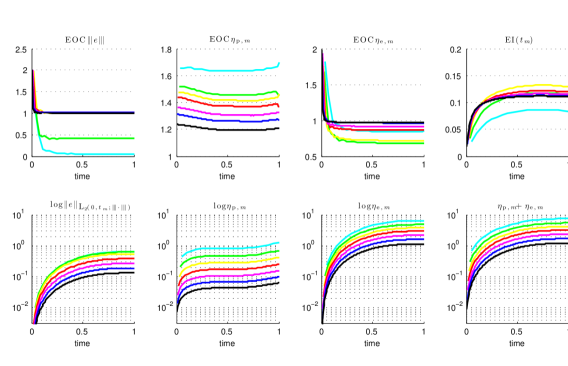
(a) Mesh-size $h(i)=2^{-i/2}$, $i=2,\dotsc,8$, and timestep $\tau=0.1\,h$. On top we plot the EOC of the single cumulative indicators $\eta_{\mathrm{p},m}$ and $\eta_{\mathrm{e},m}$. Both indicators have the same asymptotic $\operatorname{EOC}\approx 1$ as has the error. The effectivity index tends towards $1/0.12$.

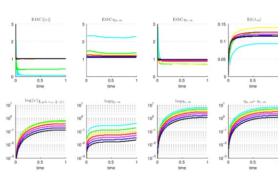
(b) Mesh-size $h(i)=2^{-i/2}$, $i=2,\dotsc,8$, and timestep $\tau=0.1\,h^{2}$. On top we plot the EOC of the single cumulative indicators $\eta_{\mathrm{p},m}$ and $\eta_{\mathrm{e},m}$. Both indicators have the same asymptotic $\operatorname{EOC}\approx 1$ as has the error. The effectivity index tends towards $1/0.12$.

Figure 2. Example (6.2) with piecewise polynomials of degree $p=2$.

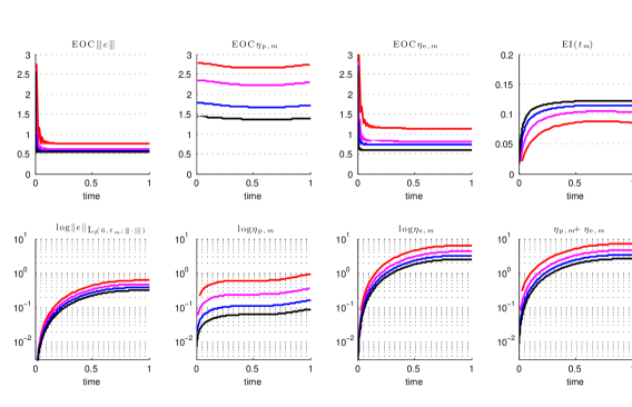
(a) Mesh-size $h(i)=2^{-i/2}$, $i=2,\dotsc,5$, and timestep $\tau=0.1\,h^{2}$. On top we plot the EOC of the single cumulative indicators $\eta_{\mathrm{p},m}$ and $\eta_{\mathrm{e},m}$. $EOC<1$ for the error is due to lack of $H^{2}$-regularity. Note that the elliptic estimator has asymptotically the same EOC as the error.

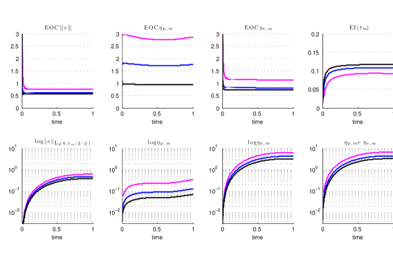
(b) Mesh-size $h(i)=2^{-i/2}$, $i=2,\dotsc,4$ and timestep $\tau=0.1h^{3}$. On top we plot the EOC of the single cumulative indicators $\eta_{\mathrm{p},m}$ and $\eta_{\mathrm{e},m}$. $EOC<1$ for the error is due to lack of $H^{2}$-regularity. Note that the elliptic estimator has asymptotically the same EOC as the error.

Figure 3. Example (6.3) with discontinuous piecewise polynomials of degree $p=3$.

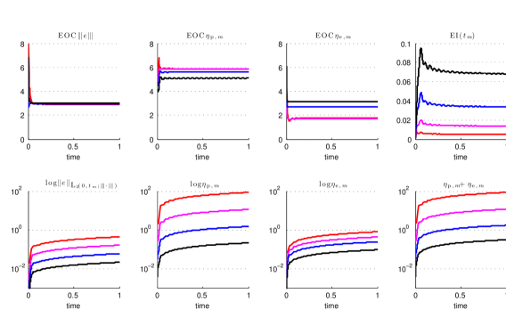
(a) Mesh-size $h(i)=2^{-i/2}$, $i=2,\dotsc,5$ and timestep $\tau=0.1\,h^{3}$. On top we plot the EOC of the single cumulative indicators $\eta_{\mathrm{p},m}$ and $\eta_{\mathrm{e},m}$. Both indicators have the same asymptotic $EOC\approx 1$ as has the error. The effectivity index tends towards asymptotic value $200$.

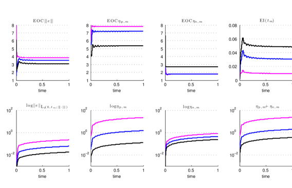
(b) Mesh-size $h(i)=2^{-i/2}$, $i=2,\dotsc,4$ and timestep $\tau=0.1\,h^{4}$. On top we plot the EOC of the single cumulative indicators $\eta_{\mathrm{p},m}$ and $\eta_{\mathrm{e},m}$. Both indicators have the same asymptotic $EOC\approx 1$ as has the error. The effectivity index tends towards asymptotic value $200$

References

- [1] M. Ainsworth, A synthesis of a posteriori error estimation techniques for conforming, non-conforming and discontinuous Galerkin finite element methods, in Recent advances in adaptive computation, vol. 383 of Contemp. Math., Amer. Math. Soc., Providence, RI, 2005, pp. 1–14.
- [2] , A posteriori error estimation for discontinuous Galerkin finite element approximation, SIAM J. Numer. Anal., 45 (2007), pp. 1777–1798 (electronic).
- [3] D. N. Arnold, An interior penalty finite element method with discontinuous elements, SIAM J. Numer. Anal., 19 (1982), pp. 742–760.
- [4] D. N. Arnold, F. Brezzi, B. Cockburn, and L. D. Marini, Unified analysis of discontinuous Galerkin methods for elliptic problems, SIAM J. Numer. Anal., 39 (2001/02), pp. 1749–1779 (electronic).
- [5] G. A. Baker, Finite element methods for elliptic equations using nonconforming elements, Math. Comp., 31 (1977), pp. 45–59.
- [6] R. Becker, P. Hansbo, and M. G. Larson, Energy norm a posteriori error estimation for discontinuous Galerkin methods, Comput. Methods Appl. Mech. Engrg., 192 (2003), pp. 723–733.
- [7] A. Bergam, C. Bernardi, and Z. Mghazli, A posteriori analysis of the finite element discretization of some parabolic equations, Math. Comp., 74 (2005), pp. 1117–1138 (electronic).
- [8] P. Binev, W. Dahmen, and R. DeVore, Adaptive finite element methods with convergence rates, Numer. Math., 97 (2004), pp. 219–268.
- [9] S.C. Brenner, T. Gudi and L.-Y. Sung, An a posteriori error estimator for a quadratic -interior penalty method for the biharmonic problem, IMA Journal of Numerical Analysis, (to appear).
- [10] E. Burman and A. Ern, Continuous interior penalty -finite element methods for advection and advection-diffusion equations, Math. Comp., 76 (2007), pp. 1119–1140 (electronic).
- [11] R. Bustinza, G. N. Gatica, and B. Cockburn, An a posteriori error estimate for the local discontinuous Galerkin method applied to linear and nonlinear diffusion problems, J. Sci. Comput., 22/23 (2005), pp. 147–185.
- [12] C. Carstensen, T. Gudi, and M. Jensen, A unifying theory of a posteriori error control for discontinuous Galerkin FEM, preprint, Humboldt Universität, Berlin, 2008.
- [13] J. M. Cascon, C. Kreuzer, R. H. Nochetto, and K. G. Siebert, Quasi-optimal convergence rate for an adaptive finite element method, tech. rep., University of Maryland, http://www.math.umd.edu/ rhn/publications.html, 2007.
- [14] Y. Chen and J. Yang, A posteriori error estimation for a fully discrete discontinuous Galerkin approximation to a kind of singularly perturbed problems, Finite Elem. Anal. Des., 43 (2007), pp. 757–770.
- [15] Z. Chen and F. Jia, An adaptive finite element algorithm with reliable and efficient error control for linear parabolic problems, Math. Comp., 73 (2004), pp. 1167–1193 (electronic).
- [16] B. Cockburn, G. E. Karniadakis, and C.-W. Shu, eds., Discontinuous Galerkin methods, Berlin, 2000, Springer-Verlag. Theory, computation and applications, Papers from the 1st International Symposium held in Newport, RI, May 24–26, 1999.
- [17] K. Eriksson and C. Johnson, Adaptive finite element methods for parabolic problems. I. A linear model problem, SIAM J. Numer. Anal., 28 (1991), pp. 43–77.
- [18] A. Ern and J. Proft, A posteriori discontinuous Galerkin error estimates for transient convection-diffusion equations, Appl. Math. Lett., 18 (2005), pp. 833–841.
- [19] A. Ern and A. F. Stephansen, A posteriori energy-norm error estimates for advection-diffusion equations approximated by weighted interior penalty methods, J. Comput. Math., 26 (2008), pp. 488–510.
- [20] A. Ern, A. F. Stephansen, and P. Zunino, A discontinuous Galerkin method with weighted averages for advection–diffusion equations with locally small and anisotropic diffusivity, IMA J. Numer. Anal., 29 (2009), pp. 235–256.
- [21] L. C. Evans, Partial differential equations, vol. 19 of Graduate Studies in Mathematics, American Mathematical Society, Providence, RI, 1998.
- [22] P. Grisvard, Singularities in Boundary Value Problems, vol. 22, Recherches en Mathématiques Appliquées, Masson, Paris, 1992.
- [23] P. Houston, D. Schötzau, and T. P. Wihler, Energy norm a posteriori error estimation of -adaptive discontinuous Galerkin methods for elliptic problems, Math. Models Methods Appl. Sci., 17 (2007), pp. 33–62.
- [24] P. Houston, C. Schwab, and E. Süli, Discontinuous -finite element methods for advection-diffusion-reaction problems, SIAM J. Numer. Anal., 39 (2002), pp. 2133–2163 (electronic).
- [25] P. Houston, E. Süli, and T. P. Wihler, A posteriori error analysis of hp-version discontinuous Galerkin finite element methods for second-order quasilinear elliptic problems, eprint Nottingham eprint 413, University of Nottingham, 2006.
- [26] O. A. Karakashian and F. Pascal, A posteriori error estimates for a discontinuous Galerkin approximation of second-order elliptic problems, SIAM J. Numer. Anal., 41 (2003), pp. 2374–2399 (electronic).
- [27] , Convergence of adaptive discontinuous Galerkin approximations of second-order elliptic problems, SIAM J. Numer. Anal., 45 (2007), pp. 641–665 (electronic).
- [28] O. A. Ladyženskaja, V. A. Solonnikov, and N. N. Ural′ceva, Linear and quasilinear equations of parabolic type, Translated from the Russian by S. Smith. Translations of Mathematical Monographs, Vol. 23, American Mathematical Society, Providence, R.I., 1967.
- [29] O. Lakkis and C. Makridakis, Elliptic reconstruction and a posteriori error estimates for fully discrete linear parabolic problems, Math. Comp., 75 (2006), pp. 1627–1658 (electronic).
- [30] O. Lakkis and T. Pryer, Gradient recovery in adaptive finite element methods for parabolic problems, IMA J. Numer. Anal. (to appear; preprint on http://arxiv.org/abs/0905.2764v2).
- [31] A. Logg, The FEniCS project, GNU Free Documentation License 1.2 http://www.fenics.org.
- [32] C. Makridakis and R. H. Nochetto, Elliptic reconstruction and a posteriori error estimates for parabolic problems, SIAM J. Numer. Anal., 41 (2003), pp. 1585–1594 (electronic).
- [33] P. Morin, R. H. Nochetto, and K. G. Siebert, Convergence of adaptive finite element methods, SIAM Rev., 44 (2002), pp. 631–658 (electronic) (2003). Revised reprint of “Data oscillation and convergence of adaptive FEM” [SIAM J. Numer. Anal. 38 (2000), no. 2, 466–488 (electronic); MR1770058 (2001g:65157)].
- [34] S. Nicaise and N. Soualem, A posteriori error estimates for a nonconforming finite element discretization of the heat equation, M2AN Math. Model. Numer. Anal., 39 (2005), pp. 319–348.
- [35] J. Nitsche, Über ein Variationsprinzip zur Lösung von Dirichlet-Problemen bei Verwendung von Teilräumen, die keinen Randbedingungen unterworfen sind, Abh. Math. Sem. Univ. Hamburg, 36 (1971), pp. 9–15. Collection of articles dedicated to Lothar Collatz on his sixtieth birthday.
- [36] M. Picasso, Adaptive finite elements for a linear parabolic problem, Comput. Methods Appl. Mech. Engrg., 167 (1998), pp. 223–237.
- [37] W. H. Reed and T. R. Hill, Triangular mesh methods for the neutron transport equation., Technical Report LA-UR-73-479, Los Alamos Scientific Laboratory, 1973.
- [38] B. Rivière and M. F. Wheeler, A discontinuous Galerkin method applied to nonlinear parabolic equations, in Discontinuous Galerkin methods (Newport, RI, 1999), vol. 11 of Lect. Notes Comput. Sci. Eng., Springer, Berlin, 2000, pp. 231–244.
- [39] B. Rivière, M. F. Wheeler, and V. Girault, Improved energy estimates for interior penalty, constrained and discontinuous Galerkin methods for elliptic problems. I, Comput. Geosci., 3 (1999), pp. 337–360 (2000).
- [40] S. Sun and M. F. Wheeler, norm a posteriori error estimation for discontinuous Galerkin approximations of reactive transport problems, J. Sci. Comput., 22/23 (2005), pp. 501–530.
- [41] R. Verfürth, A posteriori error estimates for finite element discretizations of the heat equation, Calcolo, 40 (2003), pp. 195–212.
- [42] M. F. Wheeler, An elliptic collocation-finite element method with interior penalties, SIAM J. Numer. Anal., 15 (1978), pp. 152–161.
- [43] J.-M. Yang and Y.-P. Chen, A unified a posteriori error analysis for discontinuous Galerkin approximations of reactive transport equations, J. Comput. Math., 24 (2006), pp. 425–434.