Numerical investigation of lens models with substructures using the perturbative method.

Abstract

We present a statistical study of the effects induced by substructures on the deflection potential of dark matter halos in the strong lensing regime. This investigation is based on the pertubative solution around the Einstein radius (Alard 2007) in which all the information on the deflection potential is specified by only a pair of one-dimensional functions on this ring.

Using direct comparison with ray-tracing solutions, we found that the iso-contours of lensed images predicted by the pertubative solution is reproduced with a mean error on their radial extension of less than $1\%$ — in units of the Einstein radius, for reasonable substructure masses. It demonstrates the efficiency of the approximation to track possible signatures of substructures.

We have evaluated these two fields and studied their properties for different lens configurations modelled either through massive dark matter halos from a cosmological N-body simulation, or via toy models of Monte Carlo distribution of substructures embedded in a triaxial Hernquist potential.

As expected, the angular power spectra of these two fields tend to have larger values for larger harmonic numbers when substructures are accounted for and they can be approximated by power-laws, whose values are fitted as a function of the profile and the distribution of the substructures.

1 Introduction

The cold dark matter (CDM) paradigm (Cole et al. 2005 and references therein) has led to a successful explanation of the large-scale structure in the galaxy distribution on scales 0.02 $\leq k\leq$ 0.15h Mpc^-1. The CDM power spectrum on these scales derived from large redshift surveys such as, for instance, the Anglo-Australian 2-degree Field Galaxy Redshift Survey (2dFGRS), is also consistent with the Lyman-$\alpha$ forest data in the redshift range $2\leq z\leq 4$ (Croft et al. 2002; Viel et al. 2003; Viel, Haehnelt & Springel 2004).

In spite of these impressive successes, there are still discrepancies between simulations and observations on scales $\leq$ 1 Mpc, extensively discussed in the recent literature. We may mention the sharp central density cusp predicted by simulations in dark matter halos and confirmed by the rotation curves of low surface brightness galaxies (de Blok et al. 2001) or in bright spiral galaxies (Palunas & Williams 2000; Salucci & Burkert 2000; Gentile et al. 2004). Moreover, deep surveys ($z\geq 1-2$), such as the Las Campanas Infrared Survey, HST Deep Field North and Gemini Deep Deep Survey (GDDS) are revealing an excess of massive early-type galaxies undergoing “top-down” assembly with high inferred specific star formation rates relative to predictions of the hierarchical scenario (Glazebrook et al. 2004; Cimatti, Daddi & Renzini 2006).

One problem that requires closer examination concerns the large number of sub-$L_{\ast}$ subhalos present in simulations but not observed (Kauffmann, White & Guiderdoni 1993; Moore et al. 1999; Klypin et al. 1999). This is the case of our Galaxy or M31, although there is mounting evidence for a large number of very low mass dwarfs (Belokurov et al. 2006). However, it is still unclear whether the CDM model needs to be modified to include self-interacting (Spergel & Steinhardt 2000) or warm dark matter (Bode, Ostriker & Turok 2001; Colín, Avila-Reese & Valenzuela 2000) or whether new physical mechanisms can dispel such discrepancies with the observations. For instance, gas cooling can be partly prevented by photoionization process which may inhibit star formation in the majority of subhalos (Bullock, Kravtsov & Weinberg 2001).

This “missing satellite problem” remains an ideal framework to test cosmological models. During the past years, different methods have been employed in order to study the gravitational potential of groups or clusters of galaxies, for instance through their X-ray lines emission of hot gas in the intra-cluster medium or through lensing considerations. However, while lensing directly probes the mass distribution in those objects, the other methods rely more often than not on strong hypotheses on the dynamical state of the gas and interactions between baryons and dark matter. For example, the gas is supposed to be in hydrostatical equilibrium in the gravitational potential well created by dark matter halo, while spherical symmetry is assumed. In this paper, we study the effects induced by substructures on the deflection potential of dark matter halos in the strong lensing regime. The presence of substructures follows from the capture of small satellites which have not yet been disrupted by tidal forces and/or suggests that the relaxation of halos is not totally finished.

Ray-tracing through N-body cosmological simulations suggest that substructures should have a significant impact on the formation of giant arcs. At clusters of galaxies scales, some results indicate that lensing optical depths can be enhanced (Bartelmann, Steinmetz & Weiss 1995; Fedeli et al. 2006; Horesh et al. 2005; Meneghetti et al. 2007a) whereas some other recent studies suggest that the impact on arc occurence frequency should only be mild (Hennawi et al. 2007). On the other hand, the presence of substructures changes the properties of strongly lensed images to a point that could lead to misleading inferred cluster mass properties if not properly accounted for (Meneghetti et al. 2007b). Assuming a one-to-one association of cluster subhalos in the mass range $10^{11}-10^{12.5}{\rm M}_{\odot}$ and galaxies, Natarajan, De Lucia & Springel (2007) used weak lensing techniques and found the fraction of mass in such subhalos to account for $10-20\%$ of the total cluster mass, thus in good agreement with predictions from simulations (Moore et al. 1999).

Likewise, at the scales of galaxies, strong lensing events have long been involving multiple quasars for which the impossibility of resolving the size or shape of the lensed images brought the attention toward flux ratios of conjugate images as a probe of subtructures. Depart from flux ratios expectations from a simple elliptically symmetric potential is often interpreted as a signature for local potential perturbations by substructures (Bradač et al. 2002; Dalal & Kochanek 2002; Bradač et al. 2004; Kochanek & Dalal 2004; Amara et al. 2006). It is unclear whether anomalous flux ratios actually probe “missing satellites” (Keeton, Gaudi & Petters 2003; Mao et al. 2004; Macciò et al. 2006). Due to the small source size in the case of lensed QSOs, sensitivity to microlensing events due to stars in the lens galaxy makes the interpretation less obvious. Astrometric perturbations of multiple quasars have also been considered (Chen et al. 2007) despite substantial observational limitations.

Presumably the best way out would be to consider extended sources like QSOs observed in VLBI or lensed galaxies that will be sensitive to a narrower range of scales for the pertubing potential and thus easier to interprete. New methods for inverting potential corrections that needed on top of a smooth distribution were proposed (Koopmans 2005; Suyu & Blandford 2006) but are not guaranteed to converge in all practical cases and seem to depend on the starting smooth distribution.

One interesting alternative approach is to treat all deviations from a circularly symmetrical potential as small perturbations (Alard 2007, 2008) defining the location where multiple extended images will form. Two perturbative fields, $f_{1}(\theta)$ and ${{\rm d}f_{0}(\theta)}/{{\rm d}\theta}$, can then be defined to characterize deflection potential of lenses as a function of the azimuthal angle $\theta$, near the Einstein radius. They respectively represent the radial and azimuthal derivative of the perturbated potential (see Eq. (10) below). Alard (2008) showed that these two fields have specific properties when one substructure of mass $\sim 1\%$ of the total mass is positioned near the critical lines. For instance, the ratio of their angular power spectra at harmonic number $n$ is nearly $1$. We will investigate the detailed properties of these perturbative fields by considering more realistic lenses such as dark matter halos extracted from cosmological simulations. In order to control all the free parameters (mass fraction, and shapes of subtructures for instance) and to study their relative impact on arc formation, we will also generate different families of toy halos.

This paper is organized as follows: in section 2 we present our lensing modelling; section 3 first sketches the pertubative lens solution and applies it to our simulated lenses for validation against a ray tracing algorithm; section 4 presents our main results on the statistics of perturbations, while the last section wraps up.

2 Numerical modelling

2.1 Lens model

Halos formed in cosmological simulations tend to be centrally cuspy ($\rho\sim r^{-1}$) and are generally not spherical, but have an triaxial shape. The triaxiality of these potential lenses is expected to increase significantly the number of arcs relative to spherical models (Oguri, Lee & Suto 2003 and references therein), and must be taken into account in numerical models. Thus, apart from dark matter halos extracted from cosmological simulations, we consider in this work typical lenses modelled by of a dark matter halo of total mass $M=10^{14}M_{\odot}$ with a generalized Hernquist density profile (Hernquist 1990):

$$\rho(R)=\frac{M}{2\pi}\frac{R_{s}}{R(R+R_{s})^{3}}\,,$$ (1)

where $R_{s}$ is the value of the scale radius, $R$ a triaxial radius defined by

$$R^{2}=\frac{X^{2}}{a^{2}}+\frac{Y^{2}}{b^{2}}+\frac{Z^{2}}{c^{2}}\,\,\,(c\leq b\leq 1),$$ (2)

and $c/a$ and $b/a$ the minor:major and intermediate:major axis ratio respectively. We decided to use an Hernquist profile for practical reasons. However, for direct comparison with common descriptions of halos from cosmological simulation in the literature, the Hernquist profile is related to an NFW profile (Navarro, Frenk & White, 1996; 1997) with the same dark matter mass within the virial radius $r_{200}$. Moreover, we also impose that the two profiles are identical in the inner part ($\leq R_{s}$) which can be achieved by using relation (2) between $R_{s}$ and the NFW scale radius $r_{s}$ in Springel, Di Matteo & Hernquist (2005). By convention, we use the concentration parameter $C_{\rm host}=r_{200}/r_{s}$ in the following to characterize the density profile of our lenses. For example, for typical lens at a redshift $z=0.2$, we use $R_{s}=223$ kpc which corresponds to a NFW profile with $C_{\rm host}=8.0$ (or equivalently $r_{200}=957$ kpc, $r_{s}=119$ kpc) and is consistent with values found in previous cosmological N-body simulations at the specific redshift and in the framework a the $\Lambda$CDM cosmology (Bullock et al. 2001; Dolag, Bartelmann & Perrotta 2004).

Axis ratios of each lens are randomly determined following Shaw et al. 2006: $b/a=0.817\pm 0.098$, $c/b=0.867\pm 0.067$ and $c/a=0.707\pm 0.095$. These values are in good agreement with previous findings from cosmological simulations (see for instance Warren et al. 1992; Cole & Lacey 1996, Kasun & Evrad 2005). Finally, it is worth mentioning that each halo is made of $15\times 10^{6}$ particles corresponding to a mass resolution of $6.67\times 10^{6}M_{\odot}$. However, we impose a troncation at a radius of value $5$ Mpc.

2.2 Substructures model

2.2.1 Mass function

Numerical N-body simulations show that dark matter halos contain a large number of self-bound substructures, which correspond to about 10-20% of their total mass (Moore et al. 1999). In the following, the number of substructures N_sub in the mass range $m$ – $m$+$dm$ is assumed to obey (Moore et al. 1999; Stoehr et al. 2003)

$${\rm d}N_{\rm sub}=\frac{A}{m^{1.78}}{\rm d}m\,.$$ (3)

The normalization constant $A$ is calculated by requiring the total mass in the clumps to be $15\%$ of the halo mass and by assuming subhalos masses in the range $10^{8}$ – $5\times 10^{12}$ M_⊙. The minimum number of particles in the substructures is about $15$, while the more massive ones have $45,000$ particles.

2.2.2 Radial distribution

Substructures are distributed according to the (normalized) probability distribution $p(r){\rm d}^{3}r=(\rho(r)/M_{h}){\rm d}^{3}r$, where $\rho(r)$ is assumed to have an Hernquist profile of concentration $C_{\rm sub}$, which yields the probability to find a clump at a distance $r$ within the volume element ${\rm d}^{3}r$. While the abundance of subtructures in halos of different masses has recently been extensively quantified in cosmological simulation (see for instance Vale & Ostriker 2004; Kravtsov et al. 2004; van den Bosh et al. 2007), their radial distribution is less understood. However, some studies seem to suggest their radial distribution is significantly less concentrated than that of the host halo (Ghigna et al. 1998, 2000; Colín et al. 1999; Springel et al. 2001; De Lucia et al. 2004; Gao et al. 2004; Nagai & Kravtsov 2005; Macciò et al. 2006). We will use either $C_{\rm sub}=5.0$ in good agreement with those past investigations, or $C_{\rm sub}=C_{\rm host}$ for comparison.

2.2.3 Density profiles and alignment

The stripping process caused by tidal forces seems to reduce the density of a clump at all radii and, in particular, in the central regions, producing a density profile with a central core (Hayashi et al. 2003). This process was further confirmed by simulations which found that the inner structure of subhalos are better described by density profiles shallower than NFW (Stoehr et al. 2003). However, other simulations seem to indicate that the central regions of clumps are well-represented by power law density profiles, which remain unmodified even after important tidal stripping (Kazantzidis et al. 2004a). This effect may be enhanced when star formation is taken into account since dissipation of the gas (from radiative cooling process) and subsequent star formation lead to a steeper dark matter density profile due to adiabatic contraction. To test the importance of these differences from the point of view of arcs formation, we allow for both of these possibilities: we simulate halos with clumps having a central core $\rho(r)\propto 1/(r_{0}+r)^{2}$, where $r_{0}$ defines a core radius, or a central cusp (Hernquist profile) and study how our resulting arcs would change from one option to the other. It is worth mentioning that each subhalo concentration parameter is obtained using relation (13) in Dolag et al. (2004) within the $\Lambda$CDM cosmology. However, to avoid spurious effects due to the lack of resolution, all subhalos represented by less than 200 particles will have a concentration parameter value corresponding to that of an halo made of exactly 200 particles (i.e $m=1.33\times 10^{9}M_{\odot}$). For core profiles, we follow Hayashi et al. (2003) and take a core of size $r_{0}\sim r_{s}$.

Finally, recent cosmological simulations suggest that subhalos tend to be more spherical than their host (Pereira et al. 2008; Knebe et al. 2008) and this effect can also be enhanced if halos are formed in simulations with gas cooling (Kazantzidis et al. 2004b). Moreover, the distribution of the major axes of substructures seems to be anisotropic, the majority of which pointing towards the center of mass of the host (Aubert, Pichon & Colombi 2004; Pereira et al. 2008). Although shapes and orientations of subhalos provide important constraints on structure formation and evolution, we have not studied their relative influence in this work. We reasonably think that modelling substructures by either triaxial shapes of spherical shapes won’t lead to any significant differences in our results.

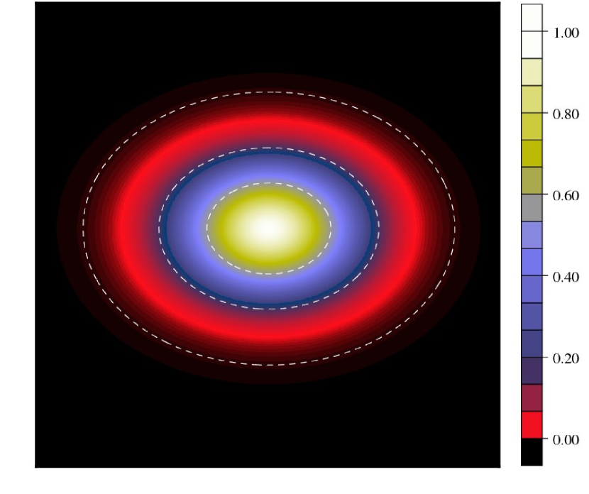
Figure 1: Elliptical luminosity contour of a source with $\eta_{0}=0.2$. The three dashed lines correspond to isophotes defined by $I(R_{1})=0.6\;I_{\rm max}$, $I(R_{2})=0.2\;I_{\rm max}$ and $I(R_{3})=0.01\;I_{\rm max}$.

2.3 Lens samples

Table 1 summarizes our different samples of lenses. From a statistical point of view, each sample involves one hundred realizations of halos following the above described methodology. Lenses are assumed to be at a typical redshift $z=0.2$. They share a common total mass of $10^{14}M_{\odot}$ and are thus described by an Hernquist profile of concentration $C=8$. The sample A represents our reference catalogue in which all halos have no substructure. For each of them, we introduce a fraction of subtructures ($F_{\rm sub}$) by removing some background particles so that both the total mass and the density profile of the initial halo are conserved. These halos are classified in catalogues B and C according the definition of inner density profile (IP) of clumps. For example, each halo from samples B1 and B2 have 15% of substructures with an inner profile represented by a cusp (Hernquist profile). Their radial distribution (RD) within the halo is left as a free parameter. We consider two possibilities, $C_{sub}=5$ as suggested by numerical simulations, and $C_{sub}=8$, which is the concentration parameter of the whole halo. Finally, lenses catalogues C1 and C2 have substructures represented by a core profile with $C_{sub}=5$ and $C_{sub}=8$ respectively.

In addition, lensing efficiency depends on the relative distance between lenses and sources. The efficiency of the lens is scaled by the critical density

$$\Sigma_{crit}=\frac{c^{2}}{4\pi G}\frac{D_{s}}{D_{d}D_{ds}},$$ (4)

where $D_{s}$, $D_{s}$ and $D_{ds}$ are the angular diameter distances between the observer and the source, between the observer and deflecting lens and between the deflector and the source respectively. When the surface mass density in the lens exceeds the critical value, multiple imaging occurs. In order to account this effect which, for a given lensing halo, implies a different Einstein radius for a different source redshift, we consider the redshift distribution of sources taken from the COSMOS sample of faint galaxies detected in the ACS/F814W band (Leauthaud et al. 2007). It is well represented by the following expression

$$\frac{{\rm d}n(z_{\rm s})}{{\rm d}z_{\rm s}}=\frac{1}{z_{0}\Gamma(a)}e^{-z_{\rm s}/z_{0}}(z_{\rm s}/z_{0})^{a-1}\;,$$ (5)

with $z_{0}=0.345$ and $a=3.89$ (Gavazzi et al. 2007).

Sample	Sub F	Sub IP	Sub RD
$A$	0%	-	-
$B1$	15%	cusp	$C_{sub}=5$
$B2$	15%	cusp	$C_{sub}=8$
$C1$	15%	core	$C_{sub}=5$
$C2$	15%	core	$C_{sub}=8$

Table 1: Samples of lenses (see details in the text).

3 numerical validation of the perturbative solution

In this section, we take advantage of the large sample of mock lenses described in § 2 to assess the validity of the perturbative method developed in (Alard 2007). After a brief presentation of the basic idea in § 3.1, we compare the ability of this simplified procedure to reproduce multiple images lensed by complex potentials as compared to a direct ray-tracing method (§ 3.3) and define the validity range of the perturbative approach.

3.1 The perturbative approach

For the sake of coherence, let us sketch the motivation behind the perturbative lens method (Alard 2007) used througout this paper. The general lens equation, relating the position of an image on the lens plane to that of the source on the source plane can be written in polar coordinates as

$${\bf r_{s}}=\Big{(}r-\frac{\partial\phi}{\partial r}\Big{)}{\bf u_{r}}-\Big{(}\frac{1}{r}\frac{\partial\phi}{\partial\theta}\Big{)}{\bf u_{\theta}}\,,$$ (6)

where $\mathbf{r}_{s}$ is the source position, and r, $\mathbf{u}_{r}$ and $\mathbf{u}_{\theta}$ are the radial distance, radial direction and orthoradial direction respectively. Here $\phi(r,\theta)$ is the projected potential. Let us now consider a lens with a projected density, $\Sigma(r)$, presenting circular symmetry, centered at the origin, and dense enough to reach critical density at the Einstein radius, $R_{E}$. Under these assumptions, the image by the lens of a point source placed at the origin is a perfect ring, and equation (6) becomes:

$$r-\frac{{\rm d}\phi_{0}}{{\rm d}r}=0,\,$$ (7)

where the potential, $\phi_{0}$, is a function of r only, and the zero subscript refers to the unperturbed solution. The basics ideas of the perturbative approach is to expand equation (7) by introducing i) small displacements of the source from the origin and ii) non-circular perturbation of the potential, $\psi$ which can be described by:

$$r_{s}=\epsilon r_{s}\,,\quad{\rm and}\quad\phi=\phi_{0}+\epsilon\psi\,,$$ (8)

where $\epsilon$ is small number: $\epsilon\ll 1$. To obtain image positions ($r$,$\theta$) by solving equation (6) directly, may prove to be analyically impossible in the general case. It is then easier to find perturbative solution by inserting equation (8) into equation (6). For convenience, we re-scale the coordinate system so that the Einstein radius is equal to unity. The response to the perturbation on $r$ may then be written as

$$r=1+\epsilon dr\,,$$ (9)

which defines $dr(\theta)$, the azimuthally dependant enveloppe of the relative deflection. Using Equation (8), the Taylor expansion of $\phi$ is

$$\phi=\phi_{0}+\epsilon\psi=\sum_{n=0}^{\infty}[C_{n}+\epsilon f_{n}(\theta)](r-1)^{n}\,,$$ (10)

where:

$$C_{n}\equiv\frac{1}{n!}\Big{[}\frac{d^{n}\phi_{0}}{dr^{n}}\Big{]}_{r=1}\,,\quad{\rm and}\quad$$ (11)

$$f_{n}(\theta)\equiv\frac{1}{n!}\Big{[}\frac{\partial^{n}\psi}{\partial r^{n}}\Big{]}_{r=1}\,.$$ (12)

Finally, inserting equations (9) and (10) into equation (6) leads to:

$${\bf r_{s}}=(\kappa_{2}{\delta}r-f_{1}){\mathbf{u}_{r}}-\frac{{\rm d}f_{0}}{{\rm d}\theta}{\bf u_{\theta}}\,,$$ (13)

with $\kappa_{2}=1-2C_{2}$. This equation corresponds to Eq. (8) in Alard (2007).

3.2 Morphological effects VS astrometric distortions

As demonstrated in Alard (2008), the morphology of arcs is very sensitive to small perturbators such as substructures in the main halo. The effect of substructures on morphological features like for instance the size of an image is typically much larger than pure astrometric distortions. Indeed, astrometric distortions are only of the order of the substructure field, which in many case is smaller than the PSF size of the instrument used, and represents then an observational challenge to measure. Note that a perturbative theory of astrometric distorsions was already considered by Kochanek et al. (2001) and Yoo et al. (2005; 2006). Note also that the former perturbative approach is limited to astrometric effects, the relevant theory does not describe image formation, and thus cannot predict morphological effects. When image morphology is considered, effects are an order of magnitude larger than astrometric effects. For instance, let us consider the examples displayed in Fig.1 and Fig. 2 of Alard (2008). Whereas a giant arc is obtained from an unperturbed elliptical lens cusp caustic (Fig. 1), the introduction near the Einstein radius of a substructure of only 1 % of the main halo mass breaks the arcs into 3 sub-images (Fig. 2). The detection of such effects should not require a particularly good resolution, since the amplitude of the effect is a fraction of the arc size, which is typically several time the PSF size.

Specifically, let us consider the following example: we take a sub-critical configuration for an elliptical lens and evaluate the modification of the image size due to the perturbation by a substructure field. Let us assume that the ellipticity of the lens is aligned with the axis system and both source and the substructure are placed on the X-axis. In this configuration, the size of the central image will be perturbed by the substructure field, and this will be the observable effect. The main interest of this example is the simplicity of the calculations (linear local description of the field) and the simple description of the effect (reduction of image size). Let us now define some useful quantities: the local slope of the unperturbed field $\alpha_{0}$, the angular size of the unperturbed image $\Delta\theta_{0}$ and the source size $R_{0}$. The substructure parameters are its mass $m_{P}$ (in unit of the main halo mass) and its distance $dr$ to the Einstein ring. For circular sources, the local slope, image size and source radius are related by the following relation in the unperturbed case:

$$\alpha_{0}\ \frac{\Delta\theta_{0}}{2}=R_{0}\,.$$ (14)

The slope perturbation introduced by the substructure $d\alpha$ is (See Alard 2008, Sec. 2):

$$d\alpha\simeq\frac{m_{P}}{dr}\,.$$ (15)

The substructure field modifies the images size according to:

$$(\alpha_{0}+d\alpha)(\Delta\theta_{0}+d\theta)=R_{0}\,,$$ (16)

which gives:

$$|d\theta|=\Delta\theta_{0}\frac{d\alpha}{\alpha_{0}}=\frac{2\ m_{P}\ R_{0}}{dr\ \alpha_{0}^{2}}\,.$$ (17)

For an elliptical isothermal potential with ellipticity parameter $\eta$, the field ${{\rm d}f_{0}(\theta)}/{{\rm d}\theta}$ reads (see Alard 2007, 2008):

$$\frac{df_{0}}{d\theta}=\eta\ \sin 2\theta-\eta\sin\theta\,.$$ (18)

Thus, $\alpha_{0}$ which is the field derivative in 0 is: $\alpha_{0}=\eta\,,$ leading to:

$$|d\theta|=2\frac{m_{P}}{dr}\frac{R_{0}}{\eta^{2}}\,.$$ (19)

The former equation evaluates the angular perturbation of the image size by the substructure. To obtain the corresponding perturbation on the image length $dS$, we have to multiply by the Einstein Radius:

$$dS\simeq R_{E}\ |d\alpha|=2R_{E}\frac{m_{P}}{dr}\frac{R_{0}}{\eta^{2}}\,.$$ (20)

Note that astrometric effects are identical to the effects of the substructure on the $f_{1}$ field for circular sources. Thus, the astrometric effect $dA$ is of the order (See Alard 2008, Sec. 2):

$$dA\simeq R_{E}\frac{m_{P}}{dr}\,.$$ (21)

Consequently, the ratio between morphological and astrometric effects here is:

$$\frac{dS}{dA}\simeq\frac{2R_{0}}{\eta^{2}}\,.$$ (22)

For arcs, the source size (source diameter= $2R_{0}$), and the parameter $\eta$ have the same typical scale, which gives: $\eta=0.1$, and $R_{0}=0.05$; then:

$$\frac{dS}{dA}\simeq 10\,.$$ (23)

This means that morphological effects are 10 times larger than astrometric effects. This point is critical, since it really makes the effect of substructure observable. To illustrate this latter point, let’s consider some numerical values for typical galaxies. For a Milky way like galaxy, we have a mass $M\simeq 6\ 10^{11}M_{\odot}$. The Einstein radius in arcsec is given by:

$$R_{E}\simeq 1.8\sqrt{\frac{M}{10^{12}M_{\odot}}}=1.4\ \ {\rm arcsec}\,,$$ (24)

which gives the size of the image perturbation, $dS=R_{E}\ |d\alpha|$:

$$dS\simeq 2.8\frac{m_{P}}{dr}\frac{R_{0}}{\eta^{2}}\ \ {\rm arcsec}\,.$$ (25)

For a perturbator with 0.5 % mass of the galaxy, taking typical scales, $dr=0.1$, $R_{0}=0.1$, and $\eta=0.1$, we obtain:

$$dS\simeq 1.4\ \ {\rm arcsec}\,.$$ (26)

Such effects should be within the reach of spatial instruments such as DUNE or SNAP. On the contrary, astrometric effects are typically 10 times smaller $dA\simeq 0.14\,\,{\rm arcsec}$ and should be then much more difficult to detect. Consequently morphological effects are definitely our best hopes to detect substructures.

Clearly, other configurations will also allow the measurement of morphological effect of substructures, though in general the calculations will be a little bit more complicated, but the effects will more or less be of the same order, since they are related to the amplitude of the perturbation of the ${{\rm d}f_{0}(\theta)}/{{\rm d}\theta}$ field by the substructure.

3.3 Reconstruction of images

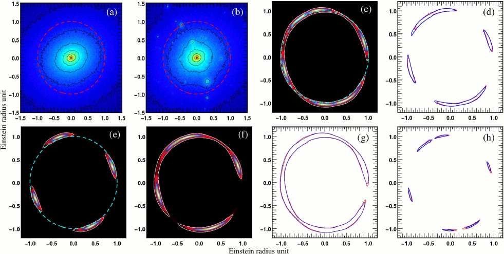
Figure 2: Projected density maps of lenses modelled by toy halos and their associated arcs reconstructions when considering an elliptical source contour with a Gaussian luminosity. Panels (a) and (e) show respectively the projected density map of the lens $L_{0}$ and the resulting image obtained from ray-tracing when the source is placed at the origin. Both red and light blue dashed lines represent the Einstein radius. The solid white line is the predicted arc reconstruction for isophotes $0.01I_{\rm max}$. Similar plots are shown in panels (b) and (f) but for $L_{3}$. Columns 3 and 4 show arc reconstructions for the lens $L_{2}$. The solution from ray-tracing is given in the panel (c) while the other last panels present a direct comparison between the isophotal contour (red) and the arc reconstruction (blue) for $0.01I_{\rm max}$ (g), $0.2I_{\rm max}$ (d) and $0.6I_{\rm max}$ (h).

One interesting feature of the perturbative method is to provide a framework for the reconstructions of images. By first defining an elliptical source centered on position $(x_{0},y_{0})$, with a characteristic size $R_{0}$, ellipticity $\sqrt{2\eta_{0}}$, and inclination of the main axis $\theta_{0}$ such that,

$$R_{0}^{2} = (1-\eta_{0}\cos\theta_{0})(x_{s}-x_{0})^{2}$$ (27)

$$+ 2\eta_{0}\sin 2\theta_{0}(x_{s}-x_{0})(y_{s}-y_{0})$$ (29)

$$+ (1+\eta_{0}\cos\theta_{0})(y_{s}-y_{0})^{2}$$ (31)

one can express the equations of the image contours using Eq. (13): (see Alard (2007) for more details)

$$dr^{\pm} = \!\!\frac{1}{\kappa_{2}}\left[\widetilde{f_{1}}+\sin 2\widetilde{\theta}\frac{\eta_{0}}{S}\frac{d\widetilde{f_{0}}}{{\rm d}\theta}\pm\frac{\sqrt{R_{0}^{2}S-(1-\eta_{0}^{2})({d\widetilde{f_{0}}}/{d\theta})^{2}}}{S}\right]$$ (32)

$$S\!\! \equiv \!\!1-\eta_{0}\cos 2\widetilde{\theta}\,,$$ (34)

$$\widetilde{\theta}\!\! \equiv \!\!\theta-\theta_{0}$$ (36)

This equation corresponds to Eq. (15) in Alard (2007). The functional $f_{i}$ is defined to take into account the effect of the translation of the source by the vector ${\bf r_{0}}=(x_{0},y_{0})$.

$$\widetilde{f_{i}}=f_{i}+x_{0}\cos\theta+y_{0}\sin\theta,\,\,\,\,{\rm for}\,\,\,\,i=0,1.$$ (37)

As emphazised in Alard (2007), the image contours are only governed by the two fields, $\widetilde{f_{1}}(\theta)$ and ${{\rm d}\widetilde{f_{0}}(\theta)}/{{\rm d}\theta}$ , which contain all the information on the deflection potential at this order in the perturbation. For instance, the two first terms in the bracket of Eq. (32) give informations on the mean position of the two contour lines while the last term provides informations on the image’s width along the radial direction as well as a condition for image formation. Therefore, the characterization of these two fields represents a simple and efficient way to track possible signatures of the deflection potential induced by substructures, so long as the perturbative framework holds, as we will illustrate below. Alard (2007) already implemented the method with a lens described by a NFW profile yielding an analytical solution for the projected potential profile. In this section, we illustrate and validate the method while considering more complicated and realistic situations. In particular, we use lenses either from cosmological simulations or from toy models presented in section 2.

For direct comparison between arc reconstructions predicted by the perturbative method and theoritical ones, we use a ray-tracing method. Part of our investigations indeed makes use of the Smooth Particle Lensing technique (SPL), described in details in Aubert, Amara & Metcalf (2007) and summarized in this section. SPL has been developed to compute the gravitational lensing signal produced by an arbitrary distribution of particles, such as the ones provided by numerical simulations. It describes particles as individual light deflectors where their surface density is arbitrarily chosen to be 2D Gaussian. This choice makes it possible to compute the analytical corresponding deflection potential, given by:

$$\phi(r)=\frac{m_{p}}{4\pi\Sigma_{c}}(\log(\frac{r^{4}}{4\sigma^{4}})-2\mathrm{Ei}(-\frac{r^{2}}{2\sigma^{2}})),$$ (38)

where $\mathrm{Ei}(x)=-\int^{\infty}_{x}\exp(-x)/x\mathrm{d}x$, $m_{p}$ is the mass of the particle, $\sigma$ its extent and $\Sigma_{c}$ the critical density. From the deflection potential, expressions for the deflection angles $\bf\alpha$, the shear components $\bf\gamma$ and the convergence $\kappa$ can be easily recovered (see Aubert, Amara & Metcalf (2007) for more details). Knowing the lensing properties of a single particle, one can recover the full signal at a given ray’s position on the sky by summing the contributions of all the individual deflectors:

$$\phi(\mathbf{r}) = \sum_{i}\phi_{i}(\mathbf{r})\,,\quad{\vec{\alpha}}(\mathbf{r})=\sum_{i}{\vec{\alpha}}_{i}(\mathbf{r})\,,$$ (39)

$$\kappa(\mathbf{r}) = \sum_{i}\kappa_{i}(\mathbf{r})\,,\quad{\vec{\gamma}}(\mathbf{r})=\sum_{i}{\vec{\gamma}}_{i}(\mathbf{r}),$$ (40)

where, e.g. $\vec{\gamma}_{i}(\mathbf{r})$ is the contribution of the i-th particle to the shear at ray’s position $\mathbf{r}$. This summations are performed efficiently by means of 2D-Tree based algorithm, in the spirit of N-body calculations. The tree calculations are restricted to monopolar approximations where an opening angle of $0.5-0.7$ is found to give results accurate at the percent level on analytical models. Finally, Aubert, Amara & Metcalf (2007) found that an adaptative resolution (i.e. an adaptative extent $\sigma$ for the particles) provides a significant improvement in the calculations in terms of accuracy. For this reason, the smoothing $\sigma$ depends on the rays location: particles shrink in high density regions in order to increase the resolution while they expand in low-density regions, smoothing the signal in undersampled areas. For all simulations, we use $1024\times 1024$ rays within a square of size $2\times 2R_{E}$, an opening angle of 0.7 and $N_{\sigma}=256$ (where $N_{\sigma}$ is the number of particles over which the smoothing is applied).

3.3.1 Lenses from the toy model

We present in this section characteristic examples of arc reconstruction. Three lenses $L_{0}$, $L_{1}$ and $L_{2}$ belonging to samples A, B2 and C2 respectively are considered. They have a common mass, density profile, axis ratios and random orientation in 3D space. They only differ via the presence or not of substructures as well as via the inner density profile of substructures: $L_{0}$ has no substructure whereas $L_{1}$ has substructures with a central cusp while a core describe the inner density profiles of substructures in $L_{2}$. In the present case, the source is at a redshift $z\sim 2.9$, has an elliptical contour with $\eta_{0}=0.2$ and a radius $R_{0}\sim 0.05R_{E}$, characterizing a Gaussian luminosity profile (see figure 1).

For the arc reconstructions presented below, we shall consider 3 different radii $R_{1}$, $R_{2}$ and $R_{3}$ corresponding to 3 specific isophotal contours defined by $I(R_{1})=0.6\;I_{\rm max}$, $I(R_{2})=0.2\;I_{\rm max}$ and $I(R_{3})=0.01\;I_{\rm max}$ (see figure 1).

In Figure (2), we show the projected mass density of lenses $L_{0}$ and $L_{1}$ near the Einstein radius, the image’s solution obtained from ray-tracing and the contours predicted by the perturbative method when the source is placed at the origin. When no substructure is considered, both projected density and potential are nearly elliptical. As expected, we obtain four distinct arcs in a cross configuration. The predicted arcs reconstruction are in good agreement with the numerical solution obtained via the ray-tracing algorithm. From a theoretical point of view, it is easy to show that the functions $\widetilde{f_{1}}(\theta)$ and ${{\rm d}\widetilde{f_{0}}(\theta)}/{{\rm d}\theta}$ are proportional to $\propto\cos(2\theta+\psi)$ and $\propto\sin(2\theta+\psi)$ respectively. These functionnal form are recovered in our experiment and shown in Figure (3).

When substructures are present, the shape of images is significantly altered. First, we notice that the positions of substructure tend to break the ellipticity of the halo center. Thus, it is not surprising that the shape of the image is approaching a ring in that case. Moreover, it is interesting to see that the position of one substructure (at the top left of the figure) is exactly at the Einstein radius. This produces an alteration of the luminosity, while the effects is more violent when substructures present a cups profile. This effect can be clearly seen when comparing the perturbative fields $\widetilde{f_{1}}(\theta)$ and ${{\rm d}\widetilde{f_{0}}(\theta)}/{{\rm d}\theta}$ relative to the lens $L_{1}$ in Figure (3). For instance, we can see two clear bumps in the evolution of ${{\rm d}\widetilde{f_{0}}(\theta)}/{{\rm d}\theta}$ . The second one ($\theta>2\pi/3$) is produced by substructures in the lower right part and induced an alteration of the luminosity again.

To estimate the systematic error between the theoretical contours provided by the ray-tracing and those predicted from equation (32), we use a simple procedure with a low computational cost. First, each predicted contour is divided into a sample of N points. Each of them is defined by polar coordinates ($r_{i}$, $\theta_{i}$) which coincide with a luminosity value of the image corresponding to an unique radius $R_{i}$ in the source frame. By using relation (32), we then compute $1+dr(R_{i})$ which gives the image contour radius of the isophotal contour $I(R_{i})$ of the source in Einstein radius unit. By defining $1+dr_{i}$ the radial distance of point i, the mean error ${\rm err}$ (in Einstein radius unit) is then computed by ${\rm err}=\sum_{i}^{N}|dr(R_{i})-dr_{i}|/{N}$.

For illustration, we have estimated the mean error reached for the lenses $L_{1}$ and $L_{2}$ using three luminosity contours source (see fig. 1). For $L_{1}$, the mean errors are respectively 0.67%, 0.71%, 0.95% of the Einstein radius for isophotes $0.6$, $0.2$ and $0.01I_{\rm max}$ respectively, while we obtain 0.74%, 0.86% and 1.04% $R_{E}$ for lens $L_{2}$ and for same luminosities. We have also studied how the mean error evolves for random positions of the source inside an area limited by the caustic lines. To do that, we have used the lens $L_{1}$ and have studied 100 realizations with different impact parameters. We found ${\rm err}=(1.01\pm 0.12)\%R_{E}$ for isophotes equal to $0.01I_{\rm max}$.

Figure 3: Variations of the fields $f_{1}$ and ${{\rm d}f_{0}(\theta)}/{{\rm d}\theta}$ as a function of $\theta$ for the lens $L_{0}$ (panels a and b), lens $L_{1}$ (panels c and d) and lens $L_{2}$ (panels e and f).

3.3.2 Lenses from cosmological simulation halos

In this section, lenses are modelled by dark matter halos extracted from a cosmological simulation of the Projet HORIZON. The simulation was run with Gadget-2 (Springel 2005) for a $\Lambda$CDM universe with $\Omega_{M}=0.3$, $\Omega_{\Lambda}=0.7$, $\Omega_{B}=0.045$, $H_{0}=70$ km/s/Mpc, $\sigma_{8}=0.92$ in a periodic box of 20 $h^{-1}$Mpc. We use $512^{3}$ particles corresponding to a mass resolution of $m_{\rm part.}\simeq 4\times 10^{6}M_{\odot}$ and a spatial resolution of 2 kpc (physical). Initial conditions has been generated from the MPgrafic code (Prunet et al. 2008), a parallel (MPI) version of Grafic (Bertschinger 2001). In this simulation, we selected two regions. In the first one, the lens is a typical halo of total mass $2.6\times 10^{13}M_{\odot}$ at redshift $z=0.5$. The source is at $z=1.2$, assumed to be elliptical ($\eta_{0}=0.2$) with $R_{0}=0.05R_{E}$ and placed near a caustic in order to obtain a giant arc. Fig. (4) shows the projected density of the lens near the Einstein radius; both the ray-tracing solution and the predicted contours by the perturbative method are shown. Here again, the three different contours are well reconstructed since the error are 0.76%, 0.83% and 0.91% $R_{E}$ for isophotes $0.6$, $0.2$ and $0.01I_{\rm max}$ respectively. For illustration, the angular variation of the perturbative fields are also representated in the figure (4).

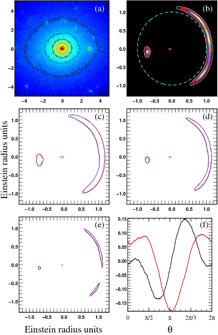
Figure 4: Projected density map (panel a) of a lens modelled by a dark matter halo extracted from the N-body simulation and the associated arc reconstructions. The solution from the ray-tracing is plotted in the panel (b) with the Einstein radius (blue line) and the predicted arc reconstruction for isophote $0.01I_{\rm max}$. The second line compares the isophote contours $0.01I_{\rm max}$ (panel c) and $0.2I_{\rm max}$ (panel d) represented by the blue lines with the predicted contour (red lines). The same results are presented in the panel e for isophote $0.6I_{\rm max}$. Finally, variations of $\widetilde{f_{1}}(\theta)$ (red line) and ${{\rm d}\widetilde{f_{0}}(\theta)}/{{\rm d}\theta}$ (black line) are plotted in the panel (f)).

The second example is a lens modelled by another halo from the same N-body simulation. Its total mass is $6.6\times 10^{13}M_{\odot}$ at $z=0.5$. This is an extreme case since a significant number of substructures are still falling toward the center of the host halo which suggests that the dynamical relaxation is still operating. This strongly affects the potential and the perturbative fields (see figure 5). However, mean errors remain small of the order of 1.11%, 1.20% and 1.26% $R_{E}$ for isophotes $0.6$, $0.2$ and $0.01I_{\rm max}$ respectively, which proves the accuracy of the method to deal with more complex systems. We may reasonably think that lenses in our different samples at $z=0.2$ tend to be more relaxed that the present configuration, and, consequently, the mean errors in our arc reconstruction should be less pronounced.

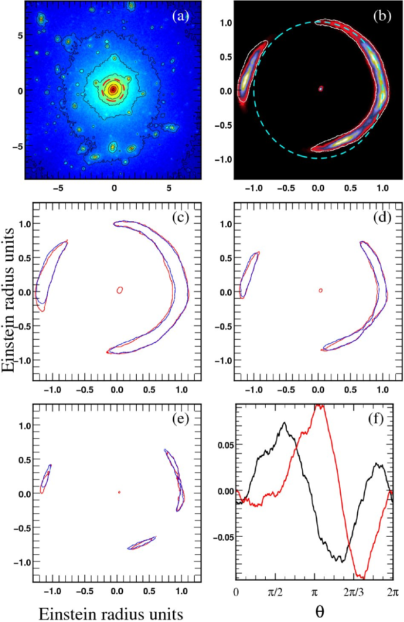
Figure 5: same as Figure 4 for another dark matter halo extracted from the N-body simulation.

4 Fourier series expansion

4.1 Motivation

Given Eq. (32), it is straightforward, for a given lensed image and an assumed underlying spherical lense and elliptical source, to invert it for $\widetilde{f_{1}}(\theta)$ and ${{\rm d}\widetilde{f_{0}}(\theta)}/{{\rm d}\theta}$ as

$$\frac{{\rm d}{\tilde{f}}_{0}}{{\rm d}\theta} = \!\!\!\frac{\pm S}{2\sqrt{1-\eta_{0}^{2}}}\sqrt{4R_{0}^{2}/S-\kappa_{2}^{2}[dr^{+}(\theta)-dr^{-}(\theta)]^{2}}$$ (41)

$${\tilde{f}}_{1}(\theta) = \!\!\!\frac{1}{2}\left(\kappa_{2}[dr^{+}(\theta)+dr^{-}(\theta)]-2\frac{{\rm d}{\tilde{f}}_{0}}{{\rm d}\theta}\frac{\eta_{0}\sin 2\widetilde{\theta}}{S}\right)\,,$$ (42)

where $S$, $\widetilde{\theta}$ and $\kappa_{2}$ are given by Eq. (32). This inversion formula depends explicitly on the source parameters, $(\eta_{0},\theta_{0})$ which are unknown. However using Eqs ( 41,  42) it is possible to compute the two functions $\widetilde{f_{1}}(\theta)$ and ${{\rm d}\widetilde{f_{0}}(\theta)}/{{\rm d}\theta}$ for each couple of parameters $(\eta_{0},\theta_{0})$. The proper solution corresponding to the true parameter $(\eta_{0},\theta_{0})$ has minimal properties. Consider for instance a circular solution ($\eta_{0}=0$), if the inversion formula is used with $\eta_{0}\neq 0$ additional Fourier terms with order $n>2$ will appear in the inversion formulae. Thus, it is clear that minimizing the power in higher order Fourier modes is a criteria that will allow to select the best solution when exploring the plane $(\eta_{0},\theta_{0})$. This criteria has also a very interesting property, considering that power at order $n>2$ usually reveal the presence of substructures (see Table 3 for instance), the solution with minimum power at higher order is also the one that puts the more robust constraint on the presence of substructure. Thus the elliptical inversion can be performed by exploring the plane $(\eta_{0},\theta_{0})$ in a given parameter range, computing the corresponding fields $\widetilde{f_{1}}(\theta)$ and ${{\rm d}\widetilde{f_{0}}(\theta)}/{{\rm d}\theta}$ and their Fourier expansion, and selecting the solution with minimum power at $n>2$. For non elliptical sources, one can use the general inversion method presented in Alard (2008). This inversion method remaps the images to the source plane using local fields models (basically the scale of the images). The solution is selected by requiring maximum similaritiy of the images in the source plane. Image similarity is evaluated by comparing the image moments up to order $N$. Provided the number of image moments equations exceed the number of model parameters, the system is closed and has a definite solution. Note that the local models may be replaced with general Fourier expansion in the interval $0<\theta<\pi$, but in this case, the additional constraint that no image are formed in dark areas must be implemented (Diego et al. 2005). In the perturbative approach this requirement can be reduced to ${{\rm d}\widetilde{f_{0}}(\theta)}/{{\rm d}\theta}$ $>R_{C}$ in dark areas, where $R_{C}$ is the radius of the smallest circular contour that contains the source. We may therefore assume for now that observational data may be inverted, and that an observationnal survey of arcs should provide us with a statistical distribution of the perturbatives fields. Hence we may use our different samples of halos presented in paragraph 2.3 in order to measure the relative influence on arc formation of the different free parameters such as the inner profile of substructures or their radial distribution within the host halo. To conduct this general analysis the fields will be represented by Fourier models, due to the direct correspondance between Fourier models of the fields and the multipolar expansion of the potential at $r=1$ (Alard 2008).

4.2 Results

The angular functions $\widetilde{f_{1}}(\theta)$ and ${{\rm d}\widetilde{f_{0}}(\theta)}/{{\rm d}\theta}$ can be characterized by their Fourier expansion:

$$\frac{d\widetilde{f_{0}}(\theta)}{{\rm d}\theta} = \sum_{n}\langle a^{0}_{n}\rangle\cos\left(n\theta+\phi^{0}_{n}\right)\,,$$ (43)

$$\widetilde{f_{1}}(\theta) = \sum_{n}\langle a^{1}_{n}\rangle\cos\left(n\theta+\phi^{1}_{n}\right)\,,$$ (44)

$$P_{i}(n) = \langle{(a^{i}_{n})}^{2}\rangle,\,\,\,\,{\rm where}\,\,\,\,i=0,1,$$ (45)

where $P_{i}(n)$, $i=1,2$ correspond to associated power spectra. We have derived the multipole expansion of $\widetilde{f_{1}}(\theta)$ and ${{\rm d}\widetilde{f_{0}}(\theta)}/{{\rm d}\theta}$ for each halo of the different catalogues and we focus in the following on the mean amplitudes $\langle a^{0}_{n}\rangle$ and $\langle a^{1}_{n}\rangle$ obtained.

Tables (2) and (3) respectively summarise the seven first orders of the power spectrum of $\widetilde{f_{1}}(\theta)$ and ${{\rm d}\widetilde{f_{0}}(\theta)}/{{\rm d}\theta}$ for the 3 lenses $L_{0}$, $L_{1}$ and $L_{2}$.

Lens	1	2	3	4	5	6	7
$L_{0}$	0.07	4.21	0.02	0.20	0.04	0.07	0.03
$L_{1}$	1.62	3.80	0.42	0.18	0.29	0.20	0.33
$L_{2}$	1.38	2.86	0.18	0.20	0.10	0.11	0.11

Table 2: Power spectra of $\widetilde{f_{1}}(\theta)$ shown in the first column of Figure 3 .

Lens	1	2	3	4	5	6	7
$L_{0}$	0.08	8.17	0.04	0.39	0.02	0.08	0.03
$L_{1}$	1.14	4.12	0.32	1.50	0.28	0.59	0.24
$L_{2}$	1.54	5.36	0.20	0.74	0.07	0.14	0.18

Table 3: Power spectra of ${{\rm d}\widetilde{f_{0}}(\theta)}/{{\rm d}\theta}$ shown in the second column of Figure 3 .

When substructures are absent, both harmonic power spectra of $\widetilde{f_{1}}(\theta)$ and ${{\rm d}\widetilde{f_{0}}(\theta)}/{{\rm d}\theta}$ are dominated by the second order mode, which is characteristic of a projected elliptical potential. The situation is totally different when substructures are taken into account. First, we notice that first mode ($n=1$) increase for lenses $L_{1}$ and $L_{2}$. This is due to the fact that we kept the same definition of the mass center between the three lenses. The random position of subtructures generates a non zero impact parameter which affect the first order mode according the relation (37). Moreover, since substructures tend to break the ellipticity of the halo center in the present case, one expects that the second mode decreases. However, the most interesting feature is that modes corresponding to $n\geq 3$ increase when substructures are present.

4.3 Practical limitations

A fraction of the error is produced by the ray-tracing simulation as well as the limitation of the considered resolution. Let us therefore consider a toy halo with an isothermal profile:

$$\rho=\frac{\rho_{0}}{r^{2}},$$ (46)

where $\rho_{0}$ is evaluated so that the mass enclosed inside a radius $r=957$ kpc is $M=10^{14}M_{\odot}$. An isothermal profile is appropriate to estimate systematic error since it leads to exact solution with the perturbative method. Here again, we have evaluated the quantity ${\rm err}$ by considering 100 realizations with different impact parameters. Sources have circular contour with $R_{0}\sim 0.05R_{E}$ and 15 millions particles have been used. For isophotes $0.6I_{\rm max}$, which is supposed to have the higher error values, we have obtained ${\rm err}=(0.30\pm 0.03)$ % $R_{E}$. Thus, in the following, we will consider that both ray-tracing method and the resolution limitation induce to a mean error of 0.3 % $R_{E}$ in contours reconstructions. Moreover, as we shall see in section 4, $\widetilde{f_{1}}(\theta)$ and ${{\rm d}\widetilde{f_{0}}(\theta)}/{{\rm d}\theta}$ can be characterized by their multipole expansion and their associated power spectrum (see equations 45). In Figure (6), we plot the amplitudes $\langle a^{0}_{n}\rangle$ and $\langle a^{1}_{n}\rangle$ as a function of n derived from the present experiments. These values for the amplitude ($\sigma\sim 0.06\%R_{E}$) correspond to a noise that we have to take into account below. For this reason, we put a confident limit to $\sim 2.0\sigma$.

In Aubert et al. 2007, the influence of smoothing $N_{\sigma}$, number of particles $N_{part}$ and opening angles $\theta$ have been extensively investigated on softened isothermal spheres. The number of particles and the models used here are similar and the parameters used in the current study can be considered as the most appropriate considering these previous tests ($N_{\sigma}=256$, $\theta=0.7$, $N_{part}=15\times 10^{9}$). For instance a re-analysis of the Aubert et al. tests case present an average error in the deflection angle of 0.3-0.4 % at the Einstein radius. Considering that the profiles and the number of particles are similar, the current error estimation is in good agreement.

In the same studies, the (inverse) magnification reconstruction was also previously tested and the critical lines fluctuates around their theoretical location because of Poisson noise and ray-shooting artefacts. By increasing the number of particles and by means of adaptive smoothing, these errors can be limited. Again, the re-analysis of these tests cases allows an estimation of the error on magnification $\mu$ of $\delta\mu/\mu\sim 0.02\mu$ close to the Einstein’s radius. The inverse magnification is obtained from the joint calculation of the convergence and the shear through the same ray-shooting technique. Hence, the error estimation does not rely on some propagation procedure but on the effective calculation and thereby includes Poisson sampling effects and ray-shoot errors.

To finish, it’s interesting to determine how the error of 0.3 % $R_{E}$ in arc reconstruction is reflected in error in the image length. Let’s consider again the configuration studied in Sect. 3.2 and taking equations (14) and (17), one obtains:

$$|d\theta|=2\Delta\theta_{0}\frac{d\alpha}{\alpha_{0}}=2\frac{d\alpha\ R_{0}}{\alpha_{0}^{2}}$$ (47)

Taking $d\alpha=0.3/100$ with the same typical value, $R_{0}=\eta=0.05$, and $\alpha_{0}=\eta=0.1$ we have:

$$|d\theta|=\frac{3}{100}$$ (48)

As in the previous calculation, the actual size of the perturbation due to the error $d_{E}$ is obtained by direct multiplication with the Einstein radius. We take the same numerical value, $R_{E}=1.4\ \ {\rm arcsec}$, thus:

$$d_{E}=0.04\ \ {\rm arcsec}$$ (49)

Given the amplitude of morphological effects, this noise is not a source of concern, but had we considered astrometric effects, this noise would become be a real problem.

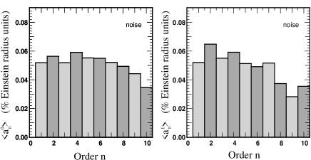
Figure 6: Variations of the mean amplitudes, $\langle a^{0}_{n}\rangle$ (left panel), and $\langle a^{1}_{n}\rangle$ (right panel), as a function of the harmonic order, $n$, derived from 100 lenses modelled by an isothermal profile.

4.4 Statistics

Figures (7) and (8) show respectively the variations of the mean amplitudes $\langle a^{0}_{n}\rangle$ and $\langle a^{1}_{n}\rangle$ as a function of $n$ derived from our different samples of lenses. As mentioned above, we put a confident limit ($\sim 2.0\sigma=0.12\%R_{E}$) and we exclude in our calculation all amplitudes below. First, when substructures are disregarded, power spectra are dominated by the second harmonic which just reflects the fact that our simulated lenses have a mean ellipticity. However, values of the fourth orders appear to be not negligible. This is probably due to the 2D projection which can lead to boxy projected densities. On the other hand, odd orders are negligible, as expected. When substructures are present, we can notice that the amplitudes of first harmonic, $\langle a^{i}_{1}\rangle$, have rather high values. As emphasized before, this is simply due to the fact the position of the lenses center is assumed to be the same for all objects. In fact, subtructures tend to modify the position of the mass center or, equivalently, tend to generate a non zero impact parameter which affect first harmonic coeficient according to the relation (37). However, the most interesting and important result is the presence of a tail in the power spectra which clearly suggests that the amplitude of high order harmonics ($n\geq 3$) are not negligible anymore. Note that these effects are clearer when the density profile of substructures is modelled by a cusp as was the case for sample $B2$. Note that the power spectra of high orders harmonic ($n\geq 3$) can be fitted by power-laws:

$$P_{0}(n\geq 3)=k_{0}n^{\alpha_{0}}\,,\quad P_{1}(n\geq 3)=k_{1}n^{\alpha_{1}}\,,$$ (50)

where the relevant fitting parameters are shown in the Table 4.

Having estimated the statistical contribution of substructures to the perturbative fields, and we may now address the problem of defining observational signatures of substructures. The observational effects are of two types: (i) an effect on the position of images which is controlled by the field $\widetilde{f_{1}}(\theta)$ , and (ii) effects on the image morphology, for instance its size in the orthoradial direction which depends on the structure of the field ${{\rm d}\widetilde{f_{0}}(\theta)}/{{\rm d}\theta}$ . An interesting point is that effects of type (i) are directly related to $\widetilde{f_{1}}(\theta)$ , while type (ii) effets is not related directly to ${{\rm d}\widetilde{f_{0}}(\theta)}/{{\rm d}\theta}$ but to its derivative (at least for images of small extension). Indeed, let us consider a source with circular contour; provided the image is small enough, a local linear expansion of the field ${{\rm d}\widetilde{f_{0}}(\theta)}/{{\rm d}\theta}$ will be sufficient to estimate the image morphology. We make the following field model:

$$\frac{d\widetilde{f_{0}}}{{\rm d}\theta}\sim\frac{{\rm d}^{2}\widetilde{f_{0}}}{{\rm d}\theta^{2}}(\theta-\theta_{0})\,,$$ (51)

where $\theta_{0}$ is a position angle which should be close to the image center. At the edge of the images, we have:

$$R_{0}=\frac{d\widetilde{f_{0}}}{{\rm d}\theta}\,.$$ (52)

By defining $\Delta\theta=\theta-\theta_{0}$, it follows that:

$$\frac{{\rm d}^{2}\widetilde{f_{0}}}{{\rm d}\theta^{2}}\Delta\theta=R_{0}\,.$$ (53)

Thus, $({{\rm d}^{2}\widetilde{f_{0}}}(\theta)/{{\rm d}\theta^{2}})^{-1}$ scales like the orthoradial image size $\Delta\theta$ and can be directly related to observational quantities. The main difference with effects of types (i), which are related to the field rather than the field derivative, is that the derivative introduce heavy weights on the higher orders of the Fourier serie expansion of the field, where the substructure contribution is dominant. Indeed, the derivative of the Fourier serie introduce a factor $n$ at order $n$, which translates in a factor $n^{2}$ on the components of the power spectrum. Thus the image morphology (and in particular its orthoradial extension for smaller images) will be much more sensitive to substructure than the average image position. To illustrate this, we have plotted in Figure (9) the amplitudes $\langle a^{0}_{n}\rangle$ for lenses samples $B1$, $B2$, $C1$ and $C2$. Moreover, to study the contribution of order $n\geq 3$, it is convenient to define the following quantities:

$${\cal P}_{1} = \langle(a^{0}_{1})^{2}\rangle+4\times\langle(a^{0}_{2})^{2}\rangle$$ (54)

$${\cal P}_{2} = \sum_{n\geq 3}n^{2}\times\langle(a^{0}_{n})^{2}\rangle$$ (56)

$$Q = \sqrt{\frac{{\cal P}_{2}}{{\cal P}_{1}}}\,,$$ (58)

Table 4 summarize mean values of $Q$ relative to each catalogue of lenses. As expected, $Q$ has higher values when substructure have a cusp profile. The total contribution of high order vary between $\sim 8$ and $18\%$ according the model of lenses used, which is quite significant.

Sample	$k_{0}$	$\alpha_{0}$	$k_{1}$	$\alpha_{1}$	$Q$
$A$	-	-	-	-	-
$B1$	3.57	-1.84	2.21	-1.69	0.113 $\pm$ 0.057
$B2$	7.33	-2.07	6.65	-2.21	0.179 $\pm$ 0.097
$C1$	0.74	-0.950	0.546	-0.845	0.083 $\pm$ 0.040
$C2$	2.08	-1.575	1.462	-1.468	0.095 $\pm$ 0.049

Table 4: Fit parameter of the statistical distribution of the harmonics of the two fields.

In closing, for the sample $C2$, mean errors between predicted contours from the perturbative method and ray-tracing solution are ${\rm err}=(0.95\pm 0.47)\%R_{E}$, ${\rm err}=(0.97\pm 0.48)\%R_{E}$ and ${\rm err}=(1.11\pm 0.49)\%R_{E}$ for isophotes $0.6$, $0.2$ and $0.01I_{\rm max}$ respectively.

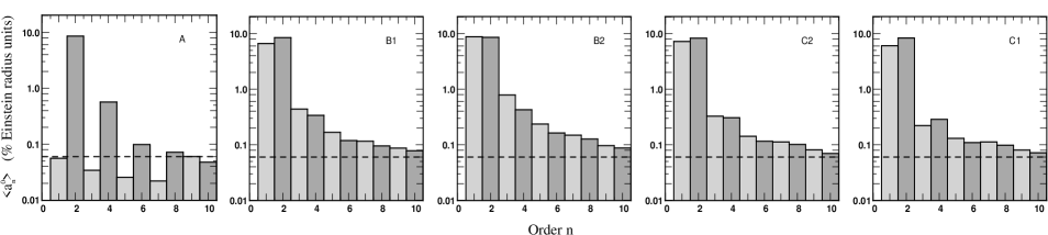
Figure 7: Variation of mean amplitudes $\langle a^{0}_{n}\rangle$ derived from multipole expansions of ${{\rm d}\widetilde{f_{0}}(\theta)}/{{\rm d}\theta}$ and for each lenses catalogue. The dashed line represent limits at $1\sigma$.

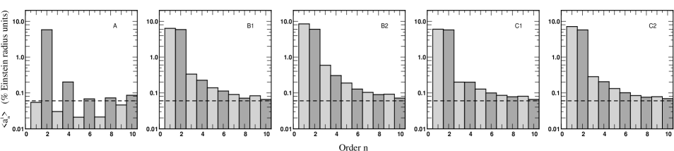
Figure 8: Variation of mean amplitudes $\langle a^{1}_{n}\rangle$ derived from multipole expansions of $\widetilde{f_{1}}(\theta)$ and for each lenses catalogue. The dashed lines represent limits at $1\sigma$.

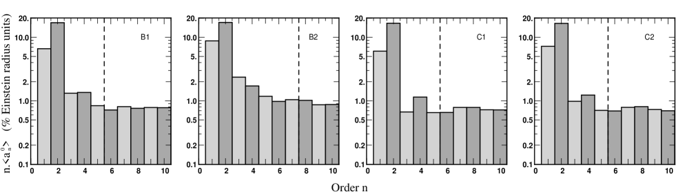
Figure 9: Variation of mean amplitudes $n\times\langle a^{0}_{n}\rangle$ for each lenses catalogue. The dashed line represents the confident limit.

5 Conclusions

The structuration of matter on galactic scales remains a privileged framework to test cosmological models. In particular, the large number of dark matter subhalos predicted by the $\Lambda$CDM cosmology is still a matter of debate. In this paper, potential signatures of substructures in the strong lensing regime were considered. This investigation makes use of the perturbative solution presented by Alard (2007, 2008), in which small deviations from the “perfect ring” configuration are treated as perturbations. In this framework, all informations on the deflection potential are contained in two one-dimensionnal fields, $f_{1}(\theta)$ and ${{\rm d}f_{0}(\theta)}/{{\rm d}\theta}$ which are related to the radial expansion of the perturbed aspherical potential. The analysis of the properties of these two fields via their harmonic decomposition represents a simple and efficient way to track back possible signatures of subtructures. For instance, the perturbative method offer a simple and clear explanation of the multiplicity of the images. As shown in Alard (2008), the unperturbed image is a long arc for a cusp caustic configuration, but when a substructure is introduced near the arc, this latter is broken in 3 images. This effect is also illustrated in the present work in the example shown in the figure (2). Basically the breaking of the image and the change in image mutiplicity is due to the perturbative terms introduced by the substructure on the field ${{\rm d}f_{0}(\theta)}/{{\rm d}\theta}$. In the case of a circular source with radius $R_{0}$, the image is broken when ${{\rm d}f_{0}(\theta)}/{{\rm d}\theta}>R_{0}$.

In this paper, lenses were modelled either by dark matter halos extracted from cosmological simulations or via toy models. The advantage of toy models is to reach a higher resolution and to allow us to study the influence of free parameters such as the inner profiles of substructures which are expected to play a central role here. We have first estimated the accuracy of the perturbative predictions by comparing the mean error between predicted contours images and theoretical ones derived via ray-tracing. We found that in general, the relative mean error is $\sim 1\%$ of the Einstein radius ($R_{E}$) when different impact parameters configurations and different source redshifts are considered. We also found that both resolution limitation and ray-tracing procedure lead to a systematic error of $\sim 0.3\%R_{E}$. Furthermore, although the accuracy of this approach for elliptical lenses is demonstrated in Alard (2007), we have checked and shown in the present study that the method works for the range of ellipticities derived from realistic 3D dark matter halos. This implies that the numerical evaluation of the coefficient of the perturbed potential, $\widetilde{f_{1}}(\theta)$ and ${{\rm d}\widetilde{f_{0}}(\theta)}/{{\rm d}\theta}$ at the Einstein radius is accurate enough to carry a statistical investigation.

We have generated several mock catalogues of lenses in which all objects have a total mass of $10^{14}M_{\odot}$ and are at redshift $z=0.2$. This value is motivated by comparison with observational surveys, and is close to where the strong lensing efficiency of clusters is the largest for sources $z_{s}\geq 1$ (Li et al. 2005). The first catalogue represents our reference sample since all lenses are modelled by dark matter halos without substructures. In the other ones, substructures are described by either a cusp profile or a core profile. Their radial distribution is also a free parameter and we have used $C_{\rm sub}=C_{\rm host}$ and $C_{\rm sub}=5$. Our statistical investigation involves a Monte-Carlo draw: the ellipticity of host halos, position of substructures, sources redshift for instance are randomly derived according to specific distributions. We found that the harmonic power spectra of $\widetilde{f_{1}}(\theta)$ and ${{\rm d}\widetilde{f_{0}}(\theta)}/{{\rm d}\theta}$ tend to develop a tail towards the large harmonics when substructure are accounted for. This effect is more pronounced when substructures have a cusp profile.

Several improvements of the present investigation are envisioned since the ultimate goal of the method is to provide a clear estimate of the amount of substructures in observations.

• Statistically, the properties of the cross-power spectrum of ${{\rm d}\widetilde{f_{0}}(\theta)}/{{\rm d}\theta}$  and $\widetilde{f_{1}}(\theta)$  will be instructive. A clear characterisation of the covariance of these fields observed in Fig. 3 along with the result of Alard (2008) upon which, as high multipole order $n$, about the same power is contained in each of the fields, would allow us to reduce the dimensionality of the problem and perhaps only consider either $\widetilde{f_{1}}(\theta)$  or ${{\rm d}\widetilde{f_{0}}(\theta)}/{{\rm d}\theta}$ .

• In this vein, it remains to be shown to which extent the statistical properties of $\widetilde{f_{1}}(\theta)$  and ${{\rm d}\widetilde{f_{0}}(\theta)}/{{\rm d}\theta}$  can be approximated as Gaussian random fields. If so, the realization of mock giant arcs would be greatly simplified. Concerning this point, the number of experiments of the present work must be increased to provide a clear diagnostic.

• A natural extension of this work would be to consider more realistic lenses while taking into account the dynamics of substructures inside the host halo, its connection to cosmology via the expected statistical distribution of substructures (see e.g. Pichon & Aubert 2006), as well as star formation mechanisms. Indeed, stripping proccesses caused by tidal forces may lead to more complex structures. For instance, the study of some merger events in the phase-space (radial velocity versus radial distance) reveals the formation of structures quite similar to caustics generated in secondary infall models of halo formation (Peirani & de Freitas Pacheco 2007). On the other hand, cooling processes and subsequent star formation may lead to steeper dark matter profile due to adiabatic contraction. Then, such processes should have an impact in the amplitude of high orders of our study.

• Obviously a perturbation of the simple circularly symmetrical case needs not lie in the same lens plane as the main deflecting halo. Uncorrelated halos superposed along the line of sight to the background source may well introduce perturbations on top of substructures belonging to the main halo. This will contribute to some additional shot noise background in the power spectra of $\widetilde{f_{1}}(\theta)$  and ${{\rm d}\widetilde{f_{0}}(\theta)}/{{\rm d}\theta}$ , which has to be quantified and subtracted off using ray-tracing through large simulated volumes. This work is beyond the scope of the present analysis.

• On the path to a possible inversion yielding $\widetilde{f_{1}}(\theta)$  and ${{\rm d}\widetilde{f_{0}}(\theta)}/{{\rm d}\theta}$  from observed arcs shapes and locations, several unknowns left on the rhs of Eq. (41) have to be controlled and will need to be fitted for in a non-linear way in order to attempt a reconstruction of fields $\widetilde{f_{1}}(\theta)$  and ${{\rm d}\widetilde{f_{0}}(\theta)}/{{\rm d}\theta}$ . In addition, we only have considered a simple representation of the background source. A lumpier background source will translate into a less regular arc with some small scale signature in the observable quantities such as ${\rm d}r_{\pm}$. However, the replication of these internal fluctuations along the arcs and, possibly, in the counter image, as well as the information contained in the various isophotes could allow us to reconstruct $\widetilde{f_{1}}(\theta)$ and ${{\rm d}\widetilde{f_{0}}(\theta)}/{{\rm d}\theta}$ directly from the observations. In this respect, Alard (2008) provides a general inversion method when two circular sources are considered for instance.

To conclude, the upcoming generation of high spatial resolution instruments dedicated to cosmology (e.g. JWST, DUNE, SNAP, ALMA) will provide us with an unprecedented number of giant arcs at all scales. The large samples expected will make standard lens modellings untractable and require the development of new methods able to capture the most relevant source of constraints for cosmology. In this respect, the perturbative method we present here may turn out to be a promising research line.

6 Acknowledgements

S. P. acknowledges the financial support through a ANR grant. This work made use of the resources available within the framework of the horizon collaboration: http://www.projet-horizon.fr. It is a pleasure to thanks T. Sousbie, K. Benabed, S. Colombi, B. Fort and G. Lavaux for interesting conversations. We thank the referee for his useful comments that helped to improve the text of this paper. We would also like to thank D. Munro for freely distributing his Yorick programming language (available at http://yorick.sourceforge.net/) which was used during the course of this work.

References

- (1) Amara A., Metcalf R. B., Cox T. J., Ostriker J. P., 2006, MNRAS, 367, 1367
- (2) Alard, C. 2007, MNRAS, 382, L58
- (3) Alard, C. 2008, MNRAS, 388, 375
- (4) Aubert, D., Amara, A., & Metcalf, R. B. 2007, MNRAS, 376, 113
- (5) Aubert, D., Pichon, C., & Colombi, S. 2004, MNRAS, 352, 376
- (6) Bartelmann, M., Steinmetz, M., & Weiss, A. 1995, A&A, 297, 1
- (7) Belokurov, V., et al. 2007, ApJ, 654, 897
- (8) Bertschinger, E. 2001, ApJS, 137, 1
- (9) Bode, P., Ostriker, J. P., & Turok, N. 2001, ApJ, 556, 93
- (10) Bradač M., Schneider P., Steinmetz M., Lombardi M., King L. J., Porcas R., 2002, A&A, 388, 373
- (11) Bradač M., Schneider P., Lombardi M., Steinmetz M., Koopmans L. V. E., Navarro J. F., 2004, A&A, 423, 797
- (12) Bullock, J. S., Kravtsov, A. V., & Weinberg, D. H. 2001, ApJ, 548, 33
- (13) Bullock, J. S., Kolatt, T. S., Sigad et al., 2001, MNRAS, 321, 559
- (14) Cimatti, A., Daddi, E., & Renzini, A. 2006, A&A, 453, L29
- (15) Chen J., Rozo E., Dalal N., Taylor J. E., 2007, ApJ, 659, 52
- (16) Cole, S., & Lacey, C. 1996, MNRAS, 281, 716
- (17) Cole, S., et al. 2005, MNRAS, 362, 505
- (18) Colín, P., Klypin, A. A., Kravtsov, A. V., & Khokhlov, A. M. 1999, ApJ, 523, 32
- (19) Colín, P., Avila-Reese, V., & Valenzuela, O. 2000, ApJ, 542, 622
- (20) Croft, R. A. C., Weinberg, D. H., Bolte, M., Burles, S., Hernquist, L., Katz, N., Kirkman, D., & Tytler, D. 2002, ApJ, 581, 20
- (21) Dalal N., Kochanek C. S., 2002, ApJ, 572, 25
- (22) de Blok W. J. G., McGaugh S. S., Bosma A. & Rubin V. C., 2001, ApJ 552, L23
- (23) De Lucia, G., Kauffmann, G., Springel, V., White, S. D. M., Lanzoni, B., Stoehr, F., Tormen, G., & Yoshida, N. 2004, MNRAS, 348, 333
- (24) Diego, J.M.,Protopapas, P., Sandvik, H.B., Tegmark, M., 2005, MNRAS, 360, 477
- (25) Dolag, K., Bartelmann, M., Perrotta et al., 2004, A&A, 416, 853
- (26) Fedeli, C., Meneghetti, M., Bartelmann, M., Dolag, K., & Moscardini, L. 2006, A&A, 447, 419
- (27) Gao, L., De Lucia, G., White, S. D. M., & Jenkins, A. 2004, MNRAS, 352, L1
- (28) Gavazzi, R., Treu, T., Rhodes, J. D., Koopmans, L. V. E., Bolton, A. S., Burles, S., Massey, R. J., & Moustakas, L. A. 2007, ApJ, 667, 176
- (29) Gentile, G., Salucci, P., Klein, U., Vergani, D., & Kalberla, P. 2004, MNRAS, 351, 903
- (30) Ghigna, S., Moore, B., Governato, F., Lake, G., Quinn, T., & Stadel, J. 1998, MNRAS, 300, 146
- (31) Ghigna, S., Moore, B., Governato, F., Lake, G., Quinn, T., & Stadel, J. 2000, ApJ, 544, 616
- (32) Glazebrook K. et al, 2004, Nat 430, 181, astro-ph/0401037
- (33) Hayashi, E., Navarro, J. F., Taylor, J. E., Stadel, J., & Quinn, T. 2003, Apj, 584, 541
- (34) Hennawi, J. F., Dalal, N., Bode, P., & Ostriker, J. P. 2007, ApJ, 654, 714
- (35) Hernquist, L. 1990, ApJ, 356, 359
- (36) Horesh, A., Ofek, E. O., Maoz, D., Bartelmann, M., Meneghetti, M., & Rix, H.-W. 2005, ApJ, 633, 768
- (37) Kasun, S. F., & Evrard, A. E. 2005, ApJ, 629, 781
- (38) Kauffmann G., White S. D. M. & Guiderdoni B., 1993, MNRAS 264, 201
- (39) Kazantzidis, S., Mayer, L., Mastropietro, C., Diemand, J., Stadel, J., & Moore, B. 2004, ApJ, 608, 663
- (40) Kazantzidis, S., Kravtsov, A. V., Zentner, A. R., Allgood, B., Nagai, D., & Moore, B. 2004, ApJL, 611, L73
- (41) Keeton C. R., Gaudi B. S., Petters A. O., 2003, ApJ, 598, 138
- (42) Klypin A., Kravtsov A. V., Valenzuela O. & Prada F., 1999, ApJ 522, 82
- (43) Knebe, A., Draganova, N., Power, C., Yepes, G., Hoffman, Y., Gottloeber, S., & Gibson, B. K. 2008, astro-ph/0802.1917
- (44) Kochanek, C. S., Keeton, C. R., & McLeod, B. A. 2001, ApJ, 547, 50
- (45) Kochanek C. S., Dalal N., 2004, ApJ, 610, 69
- (46) Koopmans L. V. E., 2005, MNRAS, 363, 1136
- (47) Kravtsov, A. V., Berlind, A. A., Wechsler, R. H., Klypin, A. A., Gottlöber, S., Allgood, B., & Primack, J. R. 2004, ApJ, 609, 35
- (48) Leauthaud, A., et al. 2007, ApJS, 172, 219
- (49) Li, G.-L., Mao, S., Jing, Y. P., Bartelmann, M., Kang, X., & Meneghetti, M. 2005, ApJ, 635, 795
- (50) Macciò A. V., Moore B., Stadel J., Diemand J., 2006, MNRAS, 366, 1529
- (51) Mao S., Jing Y., Ostriker J. P., Weller J., 2004, ApJ, 604, L5
- (52) Meneghetti M., Argazzi R., Pace F., Moscardini L., Dolag K., Bartelmann M., Li G., Oguri M., 2007a, A&A, 461, 25
- (53) Meneghetti M., Bartelmann M., Jenkins A., Frenk C., 2007b, MNRAS, 381, 171
- (54) Moore B., Ghigna S., Governato F., Lake G., Quinn T., Stadel J. & Tozzi P., 1999, ApJ 524, L19
- (55) Nagai, D., & Kravtsov, A. V. 2005, ApJ, 618, 557
- (56) Natarajan P., De Lucia G., Springel V., 2007, MNRAS, 376, 180
- (57) Navarro, J. F., Frenk, C. S., & White, S. D. M. 1996, ApJ, 462, 563
- (58) Navarro, J. F., Frenk, C. S., & White, S. D. M. 1997, ApJ, 490, 493
- (59) Oguri, M., Lee, J., & Suto, Y. 2003, ApJ, 599, 7
- (60) Palunas P. & Williams T.B., 2000, AJ 120, 2884
- (61) Peirani, S., & de Freitas Pacheco, J. A. 2007, astro-ph/0701292
- (62) Pereira, M. J., Bryan, G. L., & Gill, S. P. D. 2008, ApJ, 672, 825
- (63) Pichon, C., & Aubert, D. 2006, 368, 1657
- (64) Prunet, S., Pichon, C., Aubert, D., Pogosyan, D., Teyssier, R., & Gottloeber, S. 2008, astro-ph/0804.3536
- (65) Salucci, P., & Burkert, A. 2000, ApJl, 537, L9
- (66) Shaw, L. D., Weller, J., Ostriker, J. P., & Bode, P. 2006, ApJ, 646, 815
- (67) Spergel, D. N., & Steinhardt, P. J. 2000, Physical Review Letters, 84, 3760
- (68) Springel, V., White, S. D. M., Tormen, G., & Kauffmann, G. 2001, MNRAS, 328, 726
- (69) Springel, V., Di Matteo, T., & Hernquist, L. 2005, MNRAS, 361, 776
- (70) Springel, V. 2005, MNRAS, 364, 1105
- (71) Stoehr, F., White, S. D. M., Springel, V., Tormen, G., & Yoshida, N. 2003, MNRAS, 345, 1313
- (72) Suyu S. H., Blandford R. D., 2006, MNRAS, 366, 39
- (73) Vale A., Ostriker J. P., 2004, MNRAS, 353, 189
- (74) van den Bosch, F. C., et al. 2007, MNRAS, 376, 841
- (75) Viel M., Matarrese S., Theuns T., Munshi D. & Wang Y., 2003, MNRAS 340, L47
- (76) Viel M., Haehnelt M.G. & Springel V., 2004, MNRAS 354, 684
- (77) Warren, M. S., Quinn, P. J., Salmon, J. K., & Zurek, W. H. 1992, ApJ, 399, 405
- (78) Yoo, J., Kochanek, C. S., Falco, E. E., & McLeod, B. A. 2005, ApJ, 626, 51
- (79) Yoo, J., Kochanek, C. S., Falco, E. E., & McLeod, B. A. 2006, ApJ, 642, 22