Coherent Particle Transfer in an On-Demand Single-Electron Source

Abstract

Coherent electron transfer from a localized state trapped in a quantum dot into a ballistic conductor, taking place in on-demand electron sources, in general may result in excitation of particle-hole pairs. We consider a simple model for these effects, involving a resonance level with time-dependent energy, and derive Floquet scattering matrix describing inelastic transitions of particles in the Fermi sea. We find that, as the resonance level is driven through the Fermi level, particle transfer may take place completely without particle-hole excitations for certain driving protocols. In particular, such noiseless transfer occurs when the level moves with constant rapidity, its energy changing linearly with time. A detection scheme for studying the coherence of particle transfer is proposed.

Individual quantum states of light, supplied on demand by single-photon sources imamoglu94 ; brunel99 , are essential for current progress in manipulating and processing quantum information in quantum optics qubits . In particular, such sources are at the heart of secure transmission of quantum information by quantum cryptography bennett92 , and of quantum teleportation Bouwmeester97 . An extension of these techniques to electron systems would be crucial for the inception of fermion-based quantum information processing beenakker03 ; samuelsson04 .

While a number of elements of solid state electron optics, such as linear beamsplitters wees88 ; wharam88 and interferometers ji03 , have been known for some time, an on-demand electron source was demonstrated only recently glattli07 . In the experiment glattli07 a localized state in a quantum dot, tunnel-coupled to a ballistic conductor, was controllably charged and discharged by time-dependent modulation of the energy of the state induced by a periodic sequence of voltage pulses on the gate. In this process electrons are alternatingly, one at a time, injected in (trapped from) a quantum Hall edge channel, leading to a sequence of quantized single-electron current pulses Moskalets2008 . The energy of the injected electron could be independently controlled by tuning the out-coupling of the dot.

Yet, the nearly perfect quantization of current pulses achieved in glattli07 in general does not guarantee full quantum coherence. In a fully coherent pulse, the injected electron occupies a prescribed quantum state without accompanying particle/hole pairs excited from the Fermi sea. However, since particle/hole pairs have a finite density of states at low energy, a generic perturbation applied to a Fermi system is expected to create multiple pairs. This process, which has no analog for photon sources, constrains the protocols for generating coherent pulses.

To characterize the coherence of particle transfer, we employ an exact time-dependent (Floquet) scattering matrix, generalizing the Breit-Wigner theory of resonance scattering to arbitrary time dependence of the localized state energy $E(t)$. Applying this approach to the many-body evolution of a Fermi sea coupled to a localized state with driven energy, we identify the case of linear driving $E(t)=ct$, in which excitation creation is fully inhibited. The harmonic driving used in glattli07 is well approximated by this linear model if electron release and capture occur well within each half-period, as shown in Fig. 1 a. For such clean protocols the entanglement between injected particle and the Fermi sea is totally suppressed by Pauli blocking of multi-particle excitations.

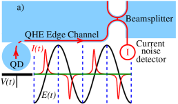
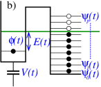
Figure 1: a) Quantum dot tunnel-coupled to a ballistic conductor. Electrons are periodically trapped on the dot and injected in the conductor as the electron energy $E(t)$ in the dot is increased above the Fermi level when a time-dependent voltage $V(t)$ is applied to the gate. Particle-hole excitations which accompany the injected electron can be detected by the current partition noise on a beamsplitter. b) Schematic diagram of a localized level coupled to a continuum of propagating modes, Eq.(1).

Clean protocols are not restricted to the adiabatic limit, and so one may study the form of clean current profiles as a function of speed of driving, which interpolates between Lorentzian when adiabatic, and exponential when fast, with fringes for intermediate rates. We also study how robust such protocols are to imperfections expected in experiment, such as noise in the driving voltage. Our results can also be relevant for quantum pumps (see Geerligs90 ; Blumenthal07 ; Moskalets02 and references therein).

A method to distinguish optimal and non-optimal protocols is illustrated in Fig. 1 a, by measuring the shot noise from current partitioning on a beamsplitter downstream of the electron source. For non-optimal protocols, the total number of excitations $N^{\mathrm{ex}}$ (electrons + holes) is greater than one. Because every electronic state scatters independently, the variance of transfered charge depends on the number of excitations that may scatter. Hence, the DC shot noise generated on the beamsplitter is $e^{2}{\sf t}(1-{\sf t})N^{\mathrm{ex}}\nu$, where ${\sf t}$ is the beamsplitter transmission coefficient and $\nu$ is the frequency of current pulses.

In the setup of Ref.glattli07 the gate used to vary $E(t)$ is placed so close to the dot that the charging energy $e^{2}/2C$ is small compared to level spacing, which allows to leave out the Hubbard-like interaction term. Also, because magnetic field of a few Tesla was applied to create a Quantum Hall state in which electron spins are polarized, only one spin projection is considered, hence electron transfer from a quantum dot to the Fermi sea is described by the many-body Hamiltonian (Fig.1 b):

$${\cal H}=E(t)d^{\dagger}d+\sum_{p}\varepsilon_{p}a^{\dagger}_{p}a_{p}+\lambda_{p}(t)d^{\dagger}a_{p}+\lambda_{p}^{\ast}(t)a_{p}^{\dagger}d$$ (1)

where $d$ and $a_{p}$ describe the localized and extended states. Here $E(t)$ is the time dependent electron energy in the dot, and $\lambda(t)$ is the tunneling amplitude, for generality also taken to be time dependent.

To describe time evolution of (1) we shall first find the single-particle scattering matrix for transitions among the continuum states $|p\rangle$. For that, we must solve the Schrödinger equations for the propagating modes $\psi_{p}(t)$ coupled to the wavefunction $\varphi(t)$ of the localized state:

$$\left[i\partial_{t}-\varepsilon_{p}\right]\psi_{p}=\lambda_{p}^{\ast}(t)\varphi,\quad\left[i\partial_{t}-E(t)\right]\varphi=\sum_{p}\lambda_{p}(t)\psi_{p}$$

(we set $\hbar=1$ and $\varepsilon_{F}=0$ unless specified otherwise). Crucially, because the localized state is coupled to the continuum at all times, its behavior (e.g. charging or discharging) can be fully accounted for by an S-matrix for transitions in the continuum. The situation here is completely analogous to the Breit-Wigner theory of resonance scattering in which an energy-dependent scattering phase is used to describe the resonance.

Because the continuum of propagating QHE modes in glattli07 is one-dimensional, it is convenient to go over to position representation $\psi(t,x)=\sum_{p}e^{ipx}\psi_{p}(t)$. Hereafter we assume a constant density of states and treat the couplings $\lambda_{p}$ as energy independent. Replacing $\varepsilon_{p}$ by $-iv_{F}\partial_{x}$, where $v_{F}$ is the Fermi velocity, gives

$$\left[i\partial_{t}-E(t)\right]\varphi(t)=\lambda(t)\int dx\delta(x)\psi(t,x)$$ (2)

$$\left[i\partial_{t}+iv_{F}\partial_{x}\right]\psi(t,x)=\lambda^{\ast}(t)\delta(x)\varphi(t).$$ (3)

The scattering matrix for energy-nonconserving time evolution can be labeled by pairs of energies of the continuum states, as $U(\varepsilon,\varepsilon^{\prime})$. Because the continuum modes propagate freely at $x<0$, the initial state is:

$$\psi(t,x<0)=\psi_{0}(t,x)=e^{-i\varepsilon^{\prime}\tilde{t}},\quad\tilde{t}=t-\frac{x}{v_{F}},$$

and $\varphi(t=-\infty)=0$ as discussed above. Projecting the evolved state onto an equivalent final state gives

$$U(\varepsilon,\varepsilon^{\prime})=\int dt\psi(t,x>0)e^{i\varepsilon\tilde{t}}.$$ (4)

Let us now solve the coupled equations of motion, and thus find $U(\varepsilon,\varepsilon^{\prime})$. First solving Eq. (3), one finds:

$$\psi(t,x)=\psi_{0}(\tilde{t})-\frac{i}{v_{F}}\lambda^{\ast}(\tilde{t})\varphi(\tilde{t})\theta(x).$$ (5)

Substituting this into Eq. (2) we find an equation for the localized state:

$$\left[i\partial_{t}-E(t)+i\frac{\gamma(t)}{2}\right]\varphi(t)=\lambda(t)\psi_{0}(t),$$ (6)

where we introduced notation $\gamma(t)=|\lambda(t)|^{2}/v_{F}$ for the localized level linewidth. Then, the solution of Eq. (6) with the initial condition $\varphi(-\infty)=0$ is of the form

$$\varphi(t)=-i\int_{-\infty}^{t}dt^{\prime}\lambda(t^{\prime})\psi_{0}(t^{\prime})e^{X(t,t^{\prime})},$$ (7)

where $X(t,t^{\prime})=-\int^{t}_{t^{\prime}}\left(\frac{1}{2}\gamma(\tau)+iE(\tau)\right)d\tau$. The result (7) may be substituted into Eq.(5) for $\psi(t,x)$; this can in turn be used in Eq. (4) to evaluate $U(\varepsilon,\varepsilon^{\prime})$. Putting all this together, we find the Floquet S-matrix

$$U(\varepsilon,\varepsilon^{\prime})=\iint dtdt^{\prime}e^{i\varepsilon t-i\varepsilon^{\prime}t^{\prime}}U(t,t^{\prime}),$$ (8)

$$U(t,t^{\prime})=\delta(t-t^{\prime})-\theta(t-t^{\prime})\frac{\lambda^{\ast}(t)\lambda(t^{\prime})}{v_{F}}e^{X(t,t^{\prime})}.$$

It is straightforward to show that $U$ is unitary, $U^{\dagger}U=\hat{1}$, by verifying that $\int U(\tau,t)U^{\ast}(\tau,t^{\prime})d\tau=\delta(t-t^{\prime})$.

As a sanity check, let us apply these results to a stationary level. For time-independent $\gamma$ and $E$, we find $X(t,t^{\prime})=-\left(\frac{\gamma}{2}+iE\right)(t-t^{\prime})$. Integrating over $t$ and $t^{\prime}$ in (8), we obtain the familiar result:

$$U(\varepsilon,\varepsilon^{\prime})=2\pi\delta(\varepsilon-\varepsilon^{\prime})\frac{\varepsilon-E-i\gamma/2}{\varepsilon-E+i\gamma/2}.$$ (9)

A more interesting example is a level moving at a constant rapidity, $E(t)=ct$. In this case, $X(t,t^{\prime})=-\frac{\gamma}{2}(t-t^{\prime})-\frac{ic}{2}(t^{2}-{t^{\prime}}^{2})$. After integrating over $t$ and $t^{\prime}$ in (8) we find $U(\varepsilon,\varepsilon^{\prime})=2\pi\delta(\varepsilon-\varepsilon^{\prime})+T(\varepsilon,\varepsilon^{\prime})$ where

$$T(\varepsilon,\varepsilon^{\prime})=-2\pi\frac{\gamma}{|c|}\theta\left(\varepsilon-\varepsilon^{\prime}\right)e^{-\frac{\gamma}{2c}(\varepsilon-\varepsilon^{\prime})+\frac{i}{2c}(\varepsilon^{2}-\varepsilon^{\prime 2})}$$ (10)

for $c>0$, and with $\theta\left(\varepsilon^{\prime}-\varepsilon\right)$ instead of $\theta\left(\varepsilon-\varepsilon^{\prime}\right)$ for $c<0$. This result agrees with the continuum limit of the Demkov-Osherov S-matrix demkov68 ; Sinitsyn2002 for a single level crossing a group of stationary levels.

We next employ this single-particle scattering matrix in the calculation of the many body properties, taking as the initial state the filled Fermi sea. The number of excitations can be obtained from the initial filled Fermi sea state $|\Omega\rangle$ evolved with the S-matrix $U(\varepsilon,\varepsilon^{\prime})$. In particular, the number of fermions promoted above the Fermi level is:

$$N^{+}=\left<\Omega\right|U^{\dagger}\!\sum_{\varepsilon>0}\!a_{\varepsilon}^{\dagger}a_{\varepsilon}U\left|\Omega\right>=\sum\limits_{\varepsilon>0,\,\varepsilon^{\prime}<0}\left|U(\varepsilon,\varepsilon^{\prime})\right|^{2}.$$ (11)

Similarly, the number of holes created below the Fermi surface $N^{-}$ is found by swapping $\varepsilon$ and $\varepsilon^{\prime}$ in Eq.(11).

Using our explicit expression for $U(\varepsilon,\varepsilon^{\prime})$ (but assuming now $\gamma(t)=\gamma$ for simplicity), one may rewrite the result (11) by using $\int_{0}^{\infty}d\varepsilon e^{i\varepsilon(t-s)}=\frac{i}{t-s+i0}$, which yields:

$$N^{+}=-\left(\frac{\gamma}{2\pi}\right)^{2}\iiiint\limits_{t>t^{\prime},\,s>s^{\prime}}\frac{e^{X(t,t^{\prime})+X^{\ast}(s,s^{\prime})}dtdt^{\prime}dsds^{\prime}}{(t-s+i0)(t^{\prime}-s^{\prime}+i0)}$$ (12)

(replacing $i0$ by $-i0$ gives an expression for $N^{-}$). It can be seen from these expressions that in general the numbers of excited particles and holes are not constrained.

To illustrate this, let us first consider a highly non-optimal protocol for E(t), where the level first moves rapidly to the Fermi-level, remains there for time $\Delta t$, and then moves rapidly away. During the time $\Delta t$, the level acts as a resonant perturbation for the Fermi sea, with scattering phase $\delta(\varepsilon)=\tan^{-1}\frac{2(\varepsilon-E)}{\gamma}-\frac{\pi}{2}$ defined by (9) This creates a logarithmically divergent number of excitations, $N^{\pm}\propto\log\Delta t$, which can be understood as an example of the “orthogonality catastrophe” Anderson67 .

The situation is completely different in the case when the level moves linearly, $E(t)=ct$. From our result for the S-matrix, Eq.(10), we have $U(\varepsilon<\varepsilon^{\prime})=0$ for $c>0$. This means that no holes are excited when the level is moving up in energy: $N^{-}=0$ for $c>0$. (Similarly when the level is moving down, i.e. $c<0$, one has $U(\varepsilon>\varepsilon^{\prime})=0$ and thus $N^{+}=0$). At the same time, we expect that $N^{+}-N^{-}=+1(-1)$ when the level moves up (down) as just one particle is transfered between the localized level and continuum. Indeed, we can find $N^{\pm}$ directly, by substituting $U$ into Eq. (11) yielding $N^{+}=1$ for $c>0$ (and $N^{-}=1$ for $c<0$). Thus for linear driving, a single fermion is coherently transfered from the localized level to the continuum, and no holes are created.

This remarkable behavior can also be understood directly from Eq. (10): restricted to $\varepsilon>0$, $\varepsilon^{\prime}<0$, $T(\varepsilon,\varepsilon^{\prime})$ is a rank one matrix. As discussed in Ref. keeling06 , for a rank one S-matrix the exact many body state is a product of an unperturbed Fermi sea and an extra particle occupying one mode, which is a superposition of harmonics with $\varepsilon>0$. The latter can be read off directly from (10):

$$\psi(t,x)=\sqrt{\frac{\gamma}{2\pi c}}\int_{0}^{\infty}\!\!d\varepsilon\,\exp\left[-i\varepsilon\tilde{t}-\frac{\gamma\varepsilon}{2c}+i\frac{\varepsilon^{2}}{2c}\right].$$ (13)

This gives a density profile $|\psi(x,t)|^{2}$ that is the convolution of a Lorentzian, width $\gamma/c$, with a Fresnel integral, leading to fringes on the trailing side of the pulse (Fig.2).

The key features of particle transfer under linear driving will be similar to that under periodic driving, used in Ref.glattli07 , if the latter sweeps a wide enough interval of energies on either side of the Fermi level. In particular, if the period is long compared to $\max(\gamma^{-1},\gamma/c)$, and the extremal value of $E(t)$ exceeds $\gamma$, as indicated in Fig.1a; then particle transfer will be nearly noiseless, close to that under linear driving. In addition, comparison to Ref.demkov68 indicates that particle transfer will remain noiseless in a more general case, when the tunnel coupling and the density of states are energy dependent, as in (1).

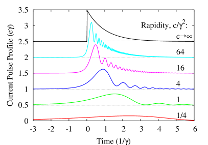
Figure 2: Single electron current pulse produced by linear driving of a localized state of width $\gamma$ across the Fermi level, $E(t)=ct$. The pulse profile $|\psi(\tilde{t})|^{2}$, $\tilde{t}=t-x/v_{F}$, Eq.(13), is shown for different values of rapidity $c$. Different curves are offset by $0.5e\gamma$. The asymptotic form is Lorentzian at slow driving, and exponential at fast driving. Note interference fringes at the trailing side of the pulse at $c\gtrsim\gamma^{2}$.

More insight into the robustness of the coherent particle transfer can be gained by considering, as an example, the effect of classical noise added to $E(t)$ (for a discussion of Landau-Zener transitions in the presence of different kinds of noise see Kayanuma98 ; Pokrovsky03 ; Wubs2006 and references therein). In experimental realizations, the energy of the localized level is not under perfect control; as well as the desired applied voltage, there will be Johnson noise and noise associated with fluctuating charges. For simplicity we consider the effect of noise on the linear driving case (see Fig. 3a):

$$E(t)=ct+\xi(t),$$ (14)

where $\left<\xi(t)\right>=0$ and $\left<\xi(t)\xi(t^{\prime})\right>=\gamma_{2}\delta(t-t^{\prime})$. Substituting this into the equation for number of excitations, Eq. (12), and averaging over realizations of the noise, we find that the integrand can be written as:

$$\frac{e^{-\frac{\gamma}{2}(t-t^{\prime}+s-s^{\prime})-\frac{ic}{2}(t^{2}-t^{\prime 2}-s^{2}+s^{\prime 2})}}{(t-s+i0)(t^{\prime}-s^{\prime}+i0)}\times F(t,t^{\prime},s,s^{\prime}),$$ (15)

where the factor $F=\langle e^{i\int_{s^{\prime}}^{s}\xi(\tau)d\tau-i\int_{t^{\prime}}^{t}\xi(\tau)d\tau}\rangle$ equals

$$\exp\left(-\frac{\gamma_{2}}{2}\left[|t-t^{\prime}|+|s-s^{\prime}|-2L(t,t^{\prime},s,s^{\prime})\right]\right).$$ (16)

Here $L(t,t^{\prime},s,s^{\prime})$ is the overlap between the two intervals $[t,t^{\prime}]$ and $[s,s^{\prime}]$ (see Fig. 3b). This simple form (16) comes from the Gaussian correlations of $\xi(\tau)$ leading to cancellation for any region inside $L(t,t^{\prime},s,s^{\prime})$.

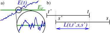
Figure 3: a) Multiple crossing of the Fermi level in the presence of noise, Eq.(14), leads to creation of particle/hole excitations; b) Overlap of time intervals and definition of $L(t,t^{\prime},s,s^{\prime})$.

To make further progress, we change variables to $s=t+\eta$, $t^{\prime}=t-\Delta_{t}$, $s^{\prime}=s-\Delta_{s}$. Because $F$ does not depend on central time $t$, the only $t$ dependence in (15) comes from $t^{2}-t^{\prime 2}-s^{2}+s^{\prime 2}=\Delta_{t}(2t-\Delta_{t})-\Delta_{s}(2t+2\eta-\Delta_{s}).$ Integration over $t$ thus gives a delta function, $\frac{2\pi}{c}\delta(\Delta_{t}-\Delta_{s})$, which considerably simplifies the expression:

$$N^{+}=\frac{-\gamma^{2}}{2\pi c}\int_{-\infty}^{\infty}\!\!\!d\eta\int_{0}^{\infty}\!\!\!d{u}\frac{e^{(-ic\eta-\gamma){u}+\gamma_{2}(L(\eta,{u})-{u})}}{(\eta+i0)^{2}},$$ (17)

(where we have written $\Delta_{t}=\Delta_{s}={u}$). In terms of $u$ and $\eta$, the overlap can be written in the simpler form: $L(\eta,{u})=\theta({u}-|\eta|)({u}-|\eta|)=u-\mathrm{min}({u},|\eta|).$ We can now examine the asymptotic limits of expression (17); for this it is convenient to consider the total number of excitations $N^{\mathrm{ex}}=N^{+}+N^{-}$. [Due to overall conservation of fermions, and assuming an initially populated localized state, $N^{+}-N^{-}=1$, as discussed above.] Combining the form of $N^{+}$ in Eq. (17) and the matching form for $N^{-}$ with $i0\to-i0$, one may use the identity $(\eta+i0)^{-2}+(\eta-i0)^{-2}=-\int_{-\infty}^{\infty}\!\!\!d\omega|\omega|e^{i\eta\omega}$. After relabeling $\omega$ to $\omega+c{u}$, we obtain

$$N^{\mathrm{ex}}=\frac{\gamma^{2}}{2\pi}\int\limits_{-\infty}^{\infty}\!\!d\omega\int\limits_{-\infty}^{\infty}\!\!d\eta\int\limits_{0}^{\infty}\!\!d{u}\,\textstyle{\left|{u}+\frac{\omega}{c}\right|}\,e^{i\omega\eta-\gamma{u}-\gamma_{2}\,\mathrm{min}({u},|\eta|)}.$$

In this form, it is easy to extract the asymptotic limits of fast and slow driving. At large $c$, we may approximate $|{u}+\omega/c|\approx{u}$. Then, integration over $\omega$ yields a delta function, $2\pi\delta(\eta)$, giving $\lim_{c\to\infty}N^{\mathrm{ex}}=1$. This limit has a simple interpretation; if driven fast enough, the effects of noise do not matter, and one recovers the clean case discussed earlier.

In the limit of small $c$, we retain only the terms proportional to $1/c$. Defining $\gamma_{\ast}=\gamma+\gamma_{2}$, we may write:

$$\int_{0}^{\infty}\!\!d{u}e^{-\gamma{u}-\gamma_{2}\,\mathrm{min}({u},|\eta|)}=\frac{1}{\gamma_{\ast}}+\frac{\gamma_{2}}{\gamma\gamma_{\ast}}e^{-\gamma^{\ast}|\eta|}$$ (18)

The integration over $\eta$ then gives

$$N^{\mathrm{ex}}=\frac{2\gamma\gamma_{2}}{\pi c}\int_{0}^{\infty}\!\!\!d\omega\frac{\omega}{\omega^{2}+\gamma_{\ast}^{2}}\approx\frac{2\gamma\gamma_{2}}{\pi c}\ln\frac{\omega_{0}}{\gamma_{\ast}}.$$ (19)

In the final expression, we have introduced a high $\omega$ cutoff $\omega_{0}$, to remove the ultraviolet divergence; this divergence corresponds to short time correlations. The origin of this divergence is the white noise spectrum for $\xi(t)$; the divergence relates to the fact that for a truly white spectrum, there will be an infinite number of crossings of the Fermi level, and so an infinite number of excitations. By comparing the fast and slow driving limits, we find the crossover occurs at the rapidity $c=(2/\pi)\gamma\gamma_{2}\ln(\omega_{0}/\gamma_{\ast})$.

In conclusion, excitation of particle/hole pairs in a single-electron source can be suppressed by optimizing the protocol of particle transfer between a localized state and continuum. The transfer is totally noiseless when the energy of the localized state varies linearly in time. In this case, owing to the Fermi statistics, particle/hole pair production is suppressed by Pauli blocking of multi-particle excitations. The quantum state resulting from such clean transfer is a product state of a particle added to an unperturbed Fermi sea, with zero entanglement between them. Particle/hole excitation, and its suppression, can be observed directly by noise measurement.

- (1) A. Imamoglu, Y. Yamamoto, Phys. Rev. Lett. 72, 210 (1994).
- (2) C. Brunel, B. Lounis, Ph. Tamarat, M. Orrit, Phys. Rev. Lett. 83, 2722 (1999).
- (3) P. Kok, et al., Rev. Mod. Phys. 79, 135 (2007).
- (4) C. H. Bennett, et al., J. Cryptology 5, 3 (1992).
- (5) D. Bouwmeester, et al., Nature 390, 575 (1997).
- (6) C. W. J. Beenakker, C. Emary, M. Kindermann, J. L. van Velsen, Phys. Rev. Lett. 91, 147901 (2003).
- (7) P. Samuelsson, E. V. Sukhorukov, M. Büttiker, Phys. Rev. Lett. 92, 026805 (2004).
- (8) B. J. van Wees, et al., Phys. Rev. Lett. 60, 848 (1988).
- (9) D. A. Wharam, et al., J. Phys. C 21, L209 (1988).
- (10) Y. Ji, et al., Nature 422, 415 (2003).
- (11) G. Fève, et al., Science 316, 1169 (2007).
- (12) M. Moskalets, P. Samuelsson, M. Buttiker, Phys. Rev. Lett. 100, 086601 (2008).
- (13) L. J. Geerligs, et al., Phys. Rev. Lett. 64, 2691 (1990).
- (14) M. D. Blumenthal, et al., Nat. Phys. 3, 343 (2007)
- (15) M. Moskalets and M. Büttiker, Phys. Rev. B66, 035306 (2002); Phys. Rev. B66, 205320 (2002).
- (16) Y. N. Demkov, V. I. Osherov, Zh. Eksp. Teor. Fiz 53, 1589 (1967) [Eng. translation: Sov. Phys. JETP 26, 916 (1968)].
- (17) N. A. Sinitsyn, Phys. Rev. B66, 205303 (2002).
- (18) P. W. Anderson, Phys. Rev. Lett. 18, 1049 (1967).
- (19) J. Keeling, I. Klich, L. S. Levitov, Phys. Rev. Lett. 97, 116403 (2006).
- (20) Y. Kayanuma, H. Nakayama, Phys. Rev. B57, 13099 (1998).
- (21) V. L. Pokrovsky, N. A. Sinitsyn, Phys. Rev. B67, 144303 (2003).
- (22) M. Wubs, K. Saito, S. Kohler, P. Hänggi, and Y. Kayanuma, Phys. Rev. Lett. 97, 200404 (2006).