Skyrmion Vibration Modes within the Rational Map Ansatz

Abstract

We study the vibration modes of the Skyrme model within the rational map ansatz. We show that the vibrations of the radial profiles and the rational maps are decoupled and we consider explicitly the case $B=1$, $B=2$ and $B=4$. We then compare our results with the vibration modes obtained numerically by Barnes et al. and show that qualitatively the rational map reproduces the vibration modes obtained numerically but that the vibration frequencies of these modes do not match very well.

1 Introduction

Proposed by Skyrme as a fundamental theory of strong interactions, the Skyrme[1] model was later shown by Witten[2] to be a low energy limit of QCD in the limit of large colour number. In that context, the classical solutions of the Skyrme model correspond to bound states of QCD. The simplest solution, with baryon number 1, can be computed analytically up to solving an ordinary differential equation numerically. For larger baryon numbers, one must compute the solutions by solving the full classical equation of the model numerically[3].

Recently, Houghton et al.[4] showed that the solution of the Skyrme model can be well approximated by the so called Rational Map ansatz. In this ansatz solutions are approximated by a radial profile function and a rational map ansatz which only depends on the polar angles variables. One then determines the radial profile by solving an ordinary differential equation while the rational map minimises an integral defined on the sphere. The configurations obtained by the ansatz fit the numerical solutions very well.

Once a classical solution has been obtained, one must still quantise some of the remaining degree of freedom. One way to do this is to compute the vibration modes of these solutions. This was done for the numerical solutions of the model by Barnes et al.[5][6] for baryon numbers $B=2$ and $4$. In this paper we compute the vibrational mode of the rational map configuration and compare them to those obtained numerically.

The Skyrme Model[1] is defined by the following Lagrangian

$$L_{p} = \int_{R^{3}}\bigg{\{}\,\frac{F_{\pi}^{2}}{16}\,Tr(\partial_{\mu}U\,\partial^{\mu}U^{{\dagger}})+\frac{1}{32e^{2}}\,Tr([(\partial_{\mu}U)\,U^{{\dagger}}\,,\,(\partial_{\nu}U)U^{{\dagger}}]^{2})$$ (1)

$$+\frac{F_{\pi}^{2}\,m_{\pi}^{2}}{8p^{2}}\,Tr(U^{p}-\mathbf{1})\bigg{\}}\,d^{3}x\;,$$

where $U=U(\vec{x},t)$ is an $SU(2)$ chiral field, $F_{\pi}$ is the pion decay constant, $m_{\pi}$ is the pion mass and $e$ a parameter of the model which is determined by fitting the classical solutions to experimental data. Notice that the last term in (1) is the so called mass term where we have used the generalised mass term proposed by Kopeliovich et al.[7] where the parameter $p$ is a positive integer.

Rather than using (1), it is convenient to rescale the space-time coordinates and the mass parameter, ${\tilde{x}_{\mu}}=2x_{\mu}/F_{\pi}e;m=m_{\pi}2/F_{\pi}e$ and use the dimensionless Lagrangian

$$L = \frac{e}{3\pi^{2}F_{\pi}}\,L_{p}$$ (2)

$$= \frac{1}{12\pi^{2}}\,\int\bigg{\{}-\frac{1}{2}Tr(R_{\mu}R^{\mu})+\frac{1}{16}Tr\Big{(}\big{[}R_{\mu},R_{\nu}\big{]}\big{[}R^{\mu},R^{\nu}\big{]}\Big{)}+\frac{m^{2}}{p^{2}}Tr\big{(}U^{p}-\mathbf{1}\big{)}\bigg{\}}\,d^{3}x\;,$$

where $R_{\mu}=(\partial_{\mu}U)U^{\dagger}$.

To approximate the solution by the rational map ansatz, we first introduce the complex coordinate $\xi=\tan(\frac{\theta}{2})\,e^{i\phi}$ where $\theta$ and $\phi$ are the polar angles. Then the rational map ansatz is given by

$$U=e^{2if(r)\,\hat{n}_{R(\xi)}\,\cdot\,\vec{\sigma}}\;,$$ (3)

where $\vec{\sigma}$ are the Pauli matrices and

$$\hat{n}_{R(\xi)}=\frac{1}{1+|R(\xi)|^{\,2}}\,\Big{(}2\Re(R(\xi)),2\Im(R(\xi)),1-|R(\xi)|^{\,2}\Big{)}\;.$$ (4)

The degree of the rational map $R(\xi)$ corresponds to the baryon number of the configuration (see [4]).

To approximate the classical solution of a given baryon number B, one would thus take

$$R(\xi)=\frac{P(\xi)}{Q(\xi)}=\frac{\sum_{i=0}^{i=B}a_{i}\xi^{i}}{\sum_{j=0}^{j=B}b_{j}\xi^{j}}$$ (5)

and insert the ansatz (3) into the Lagrangian (2). One must first determine the parameters $a_{i}$ and $b_{j}$ which minimises the integral

$$\mathcal{I} = \frac{1}{4\pi}\int\Big{(}\frac{1+|\xi|^{2}}{1+|R|^{2}}\Big{)}^{4}\;\Big{|}\frac{dR}{d\xi}\Big{|}^{\,4}\;\frac{2i\,d\xi\,\bar{d\xi}}{(1+|\xi|^{2})^{2}}\;.$$ (6)

Knowing the value of $\mathcal{I}$, one then uses the Euler-Lagrange equation to derive the equation that the profile $f(r)$ must solve. In [4], it was shown that the case $B=1$ is nothing but the hedgehog solution computed by Skyrme. For $B=2$, the configuration is axially symmetric while for $B=4$ it has the symmetry of a cube.

2 Vibration Modes

To study the vibration modes of the rational map ansatz configurations minimising (2), we add a time dependant perturbation to the rational map and the profile function around their minimising values. We then insert the perturbed ansatz into the Lagrangian (2) and compute the Euler-Lagrange equation for the perturbation, keeping only the linear terms.

Denoting $f_{0}(r)$ the minimising profile function for the static solution, we take

$$f(r,t)=f_{0}(r)+g(r,t)$$ (7)

where $g$ is assumed to be a small fluctuation around $f_{0}$ satisfying the boundary condition $g(0,t)=g(\infty,t)=0$.

To perturb a rational map, we must perturb all its coefficients, even the one that are null, by adding a small time dependant perturbation.

$$R(\xi,t)=P(\xi,t)/Q(\xi,t)$$ (8)

where

$$P(\xi,t) =\sum_{i=0}^{i=B}(a_{i}+\delta a_{i})\xi^{i}=P_{0}(\xi)+\delta P(\xi,t)$$

$$Q(\xi,t) =\sum_{j=0}^{j=B}(b_{j}+\delta b_{j})\xi^{i}=Q_{0}(\xi)+\delta Q(\xi,t)$$ (9)

Notice that, as $R$ is a ratio of $P$ and $Q$, the coefficients of the rational map are determined up to an overall constant. If $a_{B}$ is non zero, we can divide both $P$ and $Q$ by $a_{B}(1+\delta a_{B}/a_{B})$ to linear order and $\delta a_{B}$ then can be incorporated into the other $\delta a_{i}$ and $\delta b_{i}$; (if $a_{B}$ is null, one divides $P$ and $Q$ by $b_{B}(1+\delta b_{B}/b_{B})$). The rational map perturbations are thus described by $4(B+1)-2$ parameters.

When inserting (8) into (2), the perturbed rational map only occurs in the integral (6) and in the two expressions

$$\mathcal{X} = \frac{1}{4\pi}\int\frac{|\dot{R}|^{2}}{(1+|R|^{2})^{2}}\frac{2id\xi d\bar{\xi}}{(1+|\xi|^{2})^{2}}\;,$$

$$\mathcal{Y} = \frac{1}{4\pi}\int\frac{(1+|\xi|^{2})^{2}}{(1+|R|^{2})^{4}}\Big{|}\frac{dR}{d\xi}\Big{|}^{2}|\dot{R}|^{2}\frac{2id\xi d\bar{\xi}}{(1+|\xi|^{2})^{2}}\;.$$ (10)

Defining

$$\alpha_{0} = |P_{0}|^{2}+|Q_{0}|^{2}$$

$$\alpha_{1} = P_{0}(\delta\bar{P})+\bar{P}_{0}(\delta P)+Q_{0}(\delta\bar{Q})+\bar{Q}_{0}(\delta Q)$$

$$\alpha_{2} = (\delta P)(\delta\bar{P})+(\delta Q)(\delta\bar{Q})$$ (11)

$$\beta_{0} = P_{0,\,\xi}Q_{0}-P_{0}Q_{0,\,\xi}$$

$$\beta_{1} = P_{0,\,\xi}(\delta Q)-P_{0}(\delta Q)_{\xi}-Q_{0,\,\xi}(\delta P)+Q_{0}(\delta P)_{\xi}$$

$$\beta_{2} = (\delta P)_{\xi}(\delta Q)-(\delta P)(\delta Q)_{\xi}$$

$$\gamma_{0} = |\beta_{0}|^{4}$$

$$\gamma_{1} = 2\,|\beta_{0}|^{2}(\beta_{0}\bar{\beta_{1}}+\bar{\beta_{0}}\beta_{1})$$

$$\gamma_{2} = 4\,|\beta_{0}|^{2}\,|\beta_{1}|^{2}+(\beta_{0}^{2}\bar{\beta}_{1}^{2}+\bar{\beta}_{0}^{2}\beta_{1}^{2})+2\,|\beta_{0}|^{2}(\beta_{0}\bar{\beta_{2}}+\bar{\beta_{0}}\beta_{2}),$$

$$\lambda_{1} = Q_{0}(\delta\dot{P})-P_{0}(\delta\dot{Q})$$ (12)

we have

$$\mathcal{I} = \frac{1}{4\pi}\int\frac{(1+|\xi|^{2})^{2}}{\alpha_{0}^{4}}\,\bigg{[}\gamma_{0}+\Big{(}\gamma_{1}-4\gamma_{0}\frac{\alpha_{1}}{\alpha_{0}}\Big{)}$$

$$\;\;+\Big{(}10\gamma_{0}\frac{\alpha_{1}^{2}}{\alpha_{0}^{2}}-4\gamma_{0}\frac{\alpha_{2}}{\alpha_{0}}-4\gamma_{1}\frac{\alpha_{1}}{\alpha_{0}}+\gamma_{2}\Big{)}\bigg{]}\;2i\,d\xi\,\bar{d\xi}\;,$$

$$\mathcal{X} = \frac{1}{4\pi}\int\frac{|\lambda_{1}|^{2}}{\alpha_{0}^{2}}\frac{2i\,d\xi\,\bar{d\xi}}{(1+|\xi|^{2})^{2}}\;,$$

$$\mathcal{Y} = \frac{1}{4\pi}\int\frac{|\beta_{0}|^{2}|\lambda_{1}|^{2}}{\alpha_{0}^{4}}\;2i\,d\xi\,\bar{d\xi}\;,$$ (13)

Notice that the integrals (6) and (13) are at most quadratic in the parameters $\delta a$ and $\delta b$. To rewrite these integrals in matrix form, we define

$$\overrightarrow{V}(t)\equiv\left\{\begin{array}[]{c}\delta a_{i}\\ \delta b_{i}\end{array}\right\}=\left\{\begin{array}[]{c}\delta a_{0}\\ \vdots\\ \delta a_{\mathcal{B}}\\ \delta b_{0}\\ \vdots\\ \delta b_{\mathcal{B}}\end{array}\right\}\;\;\;\;\;;\;\;\;\;\;\dot{\overrightarrow{V}}(t)\equiv\left\{\begin{array}[]{c}\dot{\delta a_{i}}\\ \dot{\delta b_{i}}\end{array}\right\}=\left\{\begin{array}[]{c}\dot{\delta a_{0}}\\ \vdots\\ \\ \dot{\delta a_{\mathcal{B}}}\\ \dot{\delta b_{0}}\\ \vdots\\ \\ \dot{\delta b_{\mathcal{B}}}\end{array}\right\}\;.$$ (32)

and rewrite (13) as

$$\mathcal{I} = \mathcal{I}_{0}+\vec{V}^{T}\mathcal{I}_{2}\vec{V}$$

$$\mathcal{X} = \dot{\vec{V}^{T}}\mathcal{X}_{2}\dot{\vec{V}}$$

$$\mathcal{Y} = \dot{\vec{V}^{T}}\mathcal{Y}_{2}\dot{\vec{V}}$$ (33)

where $\mathcal{I}_{0}$ is the value of $\mathcal{I}$ for the unperturbed rational map as given in [4]. Notice that there is no linear term in $\vec{V}$. This is because the unperturbed rational map minimises (6) and (10).

Inserting the perturbed ansatz (7) and (8) into (2), we get

$$L=L_{0}+L_{2}$$ (34)

where

$$L_{0} = \frac{1}{3\pi}\int\bigg{\{}-2B\sin^{2}f_{0}-\big{(}2B\sin^{2}f_{0}+r^{2}\big{)}f_{0}^{\prime 2}-\frac{\mathcal{I}_{0}}{r^{2}}\sin^{4}f_{0}$$

$$-\frac{2m^{2}r^{2}}{p}\big{[}1-\cos(pf_{0})\big{]}\bigg{\}}\,dr\;,$$

$$L_{2} = \frac{1}{3\pi}\int\bigg{\{}4r^{2}\dot{V}_{i}\mathcal{X}_{2ij}\dot{V}_{j}\sin^{2}f_{0}+2g^{2}B\sin^{2}f_{0}-2g^{2}B\cos^{2}f_{0}$$ (35)

$$+4r^{2}\dot{V}_{i}\mathcal{X}_{2ij}\dot{V}_{j}f_{0}^{\prime 2}\sin^{2}f_{0}-2g^{\prime 2}B\sin^{2}f_{0}+2g^{2}Bf_{0}^{\prime 2}\sin^{2}f_{0}$$

$$-4gg^{\prime}Bf_{0}^{\prime}\sin(2f_{0})-2g^{2}Bf_{0}^{\prime 2}\cos^{2}f_{0}-r^{2}g^{\prime 2}+2\dot{g}^{2}B\sin^{2}f_{0}$$

$$+r^{2}\dot{g}^{2}+4\dot{V}_{i}\mathcal{Y}_{2ij}\dot{V}_{j}\sin^{4}f_{0}+\frac{2g^{2}}{r^{2}}\mathcal{I}_{0}\sin^{4}f_{0}-\frac{6g^{2}}{r^{2}}\mathcal{I}_{0}(\sin^{2}f_{0})(\cos^{2}f_{0})$$

$$-\frac{1}{r^{2}}V_{i}\mathcal{I}_{2ij}V_{j}\sin^{4}f_{0}-g^{2}m^{2}r^{2}\cos(pf_{0})\bigg{\}}\,dr\;.$$

Notice that the perturbation of the radial profile and the rational map are completely decoupled. We can thus study the radial and angular vibration modes separately. To do this we must compute the Euler-Lagrange equations for $g$ and for ${\vec{V}}$ to linear order and solve the resulting eigen value equations.

3 Rational Map Vibrations

The equation for the rational map vibrations $\vec{V}$ is straightforward to derive from (34) and can be written as

$$A_{ij}\ddot{V}_{j}=-D_{ij}V_{j}\;,$$ (36)

where

$$A_{ij} = \mathcal{X}_{2ij}\,\Gamma_{1}+\mathcal{Y}_{2ij}\,\Gamma_{2}$$

$$D_{ij} = \mathcal{I}_{2ij}\,\Gamma_{3}$$ (37)

and

$$\Gamma_{1} = \int(r^{2}\sin^{2}f_{0}+r^{2}f_{0}^{\prime 2}\sin^{2}f_{0})\,dr$$

$$\Gamma_{2} = \int(\sin^{4}f_{0})\,dr$$

$$\Gamma_{3} = \int(\frac{1}{4r^{2}}\sin^{4}f_{0})\,dr\,$$ (38)

are numerical parameters which can be evaluated numerically. We provide their value for the case $m_{\pi}=0$ and $m_{\pi}=0.526$ and $p=1$ in Tables 1 and 2.

	$B=1$	$B=2$	$B=4$
$\Gamma_{1}$	4.28869	7.58651	12.2868
$\Gamma_{2}$	0.872418	0.96429	1.02577
$\Gamma_{3}$	0.370159	0.16419	0.0895335

Table 1: $\Gamma_{1}$, $\Gamma_{2}$, $\Gamma_{3}$, for $m_{\pi}=0$

	$B=1$	$B=2$	$B=4$
$\Gamma_{1}$	3.04713	5.40344	8.94968
$\Gamma_{2}$	0.75611	0.82419	0.885387
$\Gamma_{3}$	0.405799	0.185219	0.103598

Table 2: $\Gamma_{1}$, $\Gamma_{2}$, $\Gamma_{3}$, for $m_{\pi}=0.526$ and $p=1$

To solve (36), one must first compute the matrices $\mathcal{I}_{2},\mathcal{X}_{2}$ and $\mathcal{Y}_{2}$ defined in (33). Most of the entries can be shown to vanish using parity symmetries; we have evaluated the others using both Maple and Mathematica.

Then we inserted $\vec{V}=\vec{V_{0}}\sin(\omega t)$ into (36) and used Maple and Mathematica to solve the resulting eigen value problem. We would like to point out that the eigen vectors, i.e. the vibrations, do not depend on the actual values on $\Gamma_{1}$, $\Gamma_{2}$ and $\Gamma_{3}$ (or $p$ and $m$), while the eigen values, i.e. the vibrations frequencies do. The results are described separately for the cases $B=1$, $B=2$ and $B=4$. We will then compare our results with those of Barnes et al. [5][6] obtained, in our conventions, for the value $m_{\pi}=0.526$.

3.1 B=1

For the hedgehog solution the unperturbed ration map is simply $R=\xi$ and there are 6 perturbed rational maps:

$$\begin{array}[]{lll}R_{rot,x}(\xi)=\frac{\xi+i\,d}{1+i\,d\,\xi},&R_{rot,y}(\xi)=\frac{\xi-d}{1+d\,\xi},&R_{rot,z}(\xi)=\frac{\xi}{1+i\,d},\end{array}$$ (40)

$$\begin{array}[]{lll}R_{btr,x}(\xi)=\frac{\xi+d}{1+d\,\xi},&R_{btr,y}(\xi)=\frac{\xi-i\,d}{1+i\,d\,\xi},&R_{btr,z}(\xi)=\frac{\xi}{1+d},\end{array}$$ (42)

with

$$d=\epsilon\cos(\omega t)$$ (43)

where $\epsilon$ and $\omega$ are respectively the (small) amplitude and the frequency of vibration.

$R_{rot,x}$, $R_{rot,y}$ and $R_{rot,z}$ are zero modes and correspond respectively to a rotation around the $x$, $y$ and $z$ axis. $R_{btr,x}$, $R_{btr,y}$ and $R_{btr,z}$ have the same eigen value $\omega_{btr}=0.7575$ for $m_{\pi}=0$ and $\omega_{btr}=0.9239$ for $m_{\pi}=0.526$. They form a 3 dimensional eigen space as they are conjugated to each other through a $90^{\circ}$ rotation. This eigen subspace corresponds to the broken translational invariance of the solutions: while the Skyrme Lagrangian (2) is invariant under translation, the rational map ansatz breaks that symmetry by pinning the center of the solution. If one performs the translation $x\rightarrow x+x_{0}$, into the hedgehog ansatz, the ansatz is broken, as the radial profile becomes a function of the polar angles and the rational map becomes a function of $r$. If $x_{0}$ is small, one can expand the translated expression, keeping only the linear terms in $x_{0}$. The rational map then becomes $R(\xi)=\frac{\xi+\epsilon/r}{1+\epsilon\xi/r}$. As the energy density of the Skyrmion is concentrated around a shell of radius $r_{0}$, we can take $R(\xi)=\frac{\xi+\epsilon/r_{0}}{1+\epsilon\xi/r_{0}}$ as an approximation of the translated rational map, recovering $R_{btr,x}(\xi)$. As we had to make several approximations to derive that expression of the perturbed rational map, instead of being a zero mode, it has a non zero vibration frequency that does not have any physical meaning.

We can thus conclude that, as expected, the rational map of the hedgehog solution does not have any genuine non-zero vibration mode.

3.2 B=2

The unperturbed rational map for the case $B=2$ is given by $R=\xi^{2}$ and there are 10 perturbed rational maps.

First we have the 3 rotational zero modes

$$R_{rot,x}(\xi)=\frac{\xi^{2}+i\,\epsilon\,\xi}{1+i\,\epsilon\,\xi},\qquad\qquad R_{rot,y}(\xi)=\frac{\xi^{2}-\epsilon\,\xi}{1+\epsilon\,\xi},\qquad\qquad R_{rot,z}(\xi)=\frac{\xi^{2}}{1+i\,\epsilon}.$$ (44)

Then there are 2 iso-rotation zero modes

$$R_{iso,x}(\xi)=\frac{\xi^{2}+i\,\epsilon}{1+i\,\epsilon\,\xi^{2}},\qquad\qquad R_{iso,y}(\xi)=\frac{\xi^{2}-\epsilon}{1+\epsilon\,\xi^{2}}.$$ (45)

There are only 2 such modes because the iso-rotation around the $z$ axis coincides with the proper rotation around the $z$ axis.

The lowest vibration modes are

$$R_{btr,x}(\xi)=\frac{\xi^{2}+\epsilon\,\xi}{1+\epsilon\,\xi},\qquad\qquad R_{btr,y}(\xi)=\frac{\xi^{2}-i\,\epsilon\,\xi}{1+i\,\epsilon\,\xi},\qquad\qquad R_{btr,z}(\xi)=\frac{\xi^{2}}{1+\epsilon},$$ (46)

but they correspond to the broken translation modes. Their eigen values $\omega_{btr}$ are respectively $0.69$, $0.69$ and $0.4766$ for $m_{\pi}=0$ and $0.847$ $0.847$ and $0.584$ for $m_{\pi}=0.526$, but they have no physical meaning.

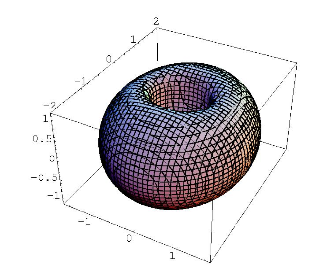
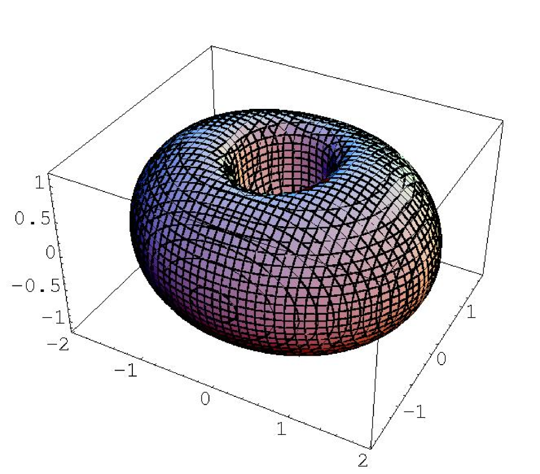
Figure 1: $B=2$, $R_{s1}(\xi)$: (Left) $\epsilon>0$; (Right) $\epsilon<0$.

We are thus left with a 2 parameter class of genuine vibration modes:

$$R_{s1}(\xi)=\frac{\xi^{2}+\epsilon}{1+\epsilon\,\xi^{2}},\qquad\qquad R_{s2}(\xi)=\frac{\xi^{2}-i\,\epsilon\,}{1+i\,\epsilon\,\xi^{2}}.$$ (47)

These two perturbed rational maps correspond to lateral squeezing and stretching of the torus alternating between elongations along the $x$ and $y$ axis as shown in Figure 1. This mode is sometimes referred to as the scattering mode as it corresponds to two Skyrmions colliding with each other. $R_{s2}$ corresponds to the same deformation but rotated by $45^{\circ}$. By taking a linear combination of $R_{s1}$ and $R_{s2}$ the torus can be made to wobble along any axis in the $x-y$ plane. The eigen value for these 2 modes is $\omega_{s}=0.9909$ for $m_{\pi}=0$ and $\omega_{s}=1.2255$ for $m_{\pi}=0.526$.

3.3 B=4

The unperturbed rational map for the case $B=4$ is given by $R=P_{0}/Q_{0}$ where $P_{0}=\xi^{4}+2\sqrt{3}\;i\;\xi^{2}+1$ and $Q_{0}=\xi^{4}-2\sqrt{3}\;i\;\xi^{2}+1$. There are 18 perturbed rational maps, including 6 zero modes:

$$R_{rot,x}(\xi) = \frac{P_{0}+(2i\,\theta_{x}-2\sqrt{3}\;\theta_{x})\xi^{3}+(2i\,\theta_{x}-2\sqrt{3}\;\theta_{x})\xi}{Q_{0}+(2i\,\theta_{x}+2\sqrt{3}\;\theta_{x})\xi^{3}+(2i\,\theta_{x}+2\sqrt{3}\;\theta_{x})\xi},$$

$$R_{rot,y}(\xi) = \frac{P_{0}+(2\sqrt{3}\;i\,\theta_{y}-2\theta_{y})\xi^{3}+(-2\sqrt{3}\;i\,\theta_{y}+2\theta_{y})\xi}{Q_{0}+(-2\sqrt{3}\;i\,\theta_{y}-2\theta_{y})\xi^{3}+(2\sqrt{3}\;i\,\theta_{y}+2\theta_{y})\xi},$$

$$R_{rot,z}(\xi) = \frac{P_{0}+4\sqrt{3}\;\theta_{z}\;\xi^{2}-4\;i\,\theta_{z}}{Q_{0}-4\sqrt{3}\;\theta_{z}\;\xi^{2}-4\;i\,\theta_{z}},$$

$$R_{iso,x}(\xi) = \frac{P_{0}+2\sqrt{3}\theta_{1}\,\xi^{2}}{Q_{0}-2\sqrt{3}\theta_{1}\,\xi^{2}},$$

$$R_{iso,y}(\xi) = \frac{P_{0}-2\sqrt{3}\,i\theta_{2}\,\xi^{2}}{Q_{0}-\theta_{2}\xi^{4}-\theta_{2}},$$

$$R_{iso,z}(\xi) = \frac{P_{0}\cdot(1+i\theta_{3})}{Q_{0}},$$ (48)

which correspond to the 3 rotations $R_{rot,x}$, $R_{rot,y}$ and $R_{rot,z}$ and 3 iso-rotations $R_{iso,x}$, $R_{iso,y}$ and $R_{iso,z}$.

The lowest vibration modes are the broken translation

$$R_{btr,x}(\xi) = \frac{P_{0}-(\frac{1}{2}+\frac{\sqrt{3}\,i}{2})\,\epsilon\,\xi^{3}-(\frac{1}{2}+\frac{\sqrt{3}\,i}{2})\,\epsilon\,\xi}{Q_{0}-(\frac{1}{2}-\frac{\sqrt{3}\,i}{2})\epsilon\,\xi^{3}-(\frac{1}{2}-\frac{\sqrt{3}\,i}{2})\,\epsilon\,\xi},$$

$$R_{btr,y}(\xi) = \frac{P_{0}-(\frac{\sqrt{3}}{2}+\frac{i}{2})\,\epsilon\,\xi^{3}+(\frac{\sqrt{3}}{2}+\frac{i}{2})\,\epsilon\,\xi}{Q_{0}+(\frac{\sqrt{3}}{2}-\frac{i}{2})\epsilon\,\xi^{3}-(\frac{\sqrt{3}}{2}-\frac{i}{2})\,\epsilon\,\xi},$$

$$R_{btr,z}(\xi) = \frac{P_{0}+\sqrt{3}\,i\,\epsilon\,\xi^{2}+\epsilon\,}{Q_{0}-\sqrt{3}\,i\,\epsilon\,\xi^{2}+\epsilon}$$ (49)

and their eigen values are $\omega_{tr}=0.4586$ for $m_{\pi}=0$ and $\omega_{tr}=0.5625$ for $m_{\pi}=0.526$.

The first genuine vibration mode is given by

$$R_{tb,x}(\xi) = \frac{P_{0}-(\frac{\sqrt{3}}{2}-\frac{i}{2})\,\epsilon\,\xi^{3}-(\frac{\sqrt{3}}{2}-\frac{i}{2})\,\epsilon\,\xi}{Q_{0}-(\frac{\sqrt{3}}{2}+\frac{i}{2})\epsilon\,\xi^{3}-(\frac{\sqrt{3}}{2}+\frac{i}{2})\,\epsilon\,\xi},$$

$$R_{tb,y}(\xi) = \frac{P_{0}-(\frac{1}{2}-\frac{\sqrt{3}\,i}{2})\,\epsilon\,\xi^{3}+(\frac{1}{2}-\frac{\sqrt{3}\,i}{2})\,\epsilon\,\xi}{Q_{0}+(\frac{1}{2}+\frac{\sqrt{3}\,i}{2})\epsilon\,\xi^{3}-(\frac{1}{2}+\frac{\sqrt{3}\,i}{2})\,\epsilon\,\xi},$$

$$R_{tb,z}(\xi) = \frac{P_{0}+\sqrt{3}\,\epsilon\,\xi^{2}-i\,\epsilon}{Q_{0}-i\,\epsilon\,\xi^{4}-\sqrt{3}\,\epsilon\,\xi^{2}}$$ (50)

and its eigen value is $\omega_{tb}=0.6093$ for $m_{\pi}=0$ and $\omega_{tb}=0.7508$ for $m_{\pi}=0.526$. To picture it one, has to think of the cube as two tori stacked on top of each other. Then each torus oscillates like the scattering mode of the $B=2$ solution but in phase opposition. This results in a cube which is somewhat squeezed into a toroidal shape as shown in figure 2. This can also be thought of as the scattering of four Skyrmions in a tetrahedral configuration.

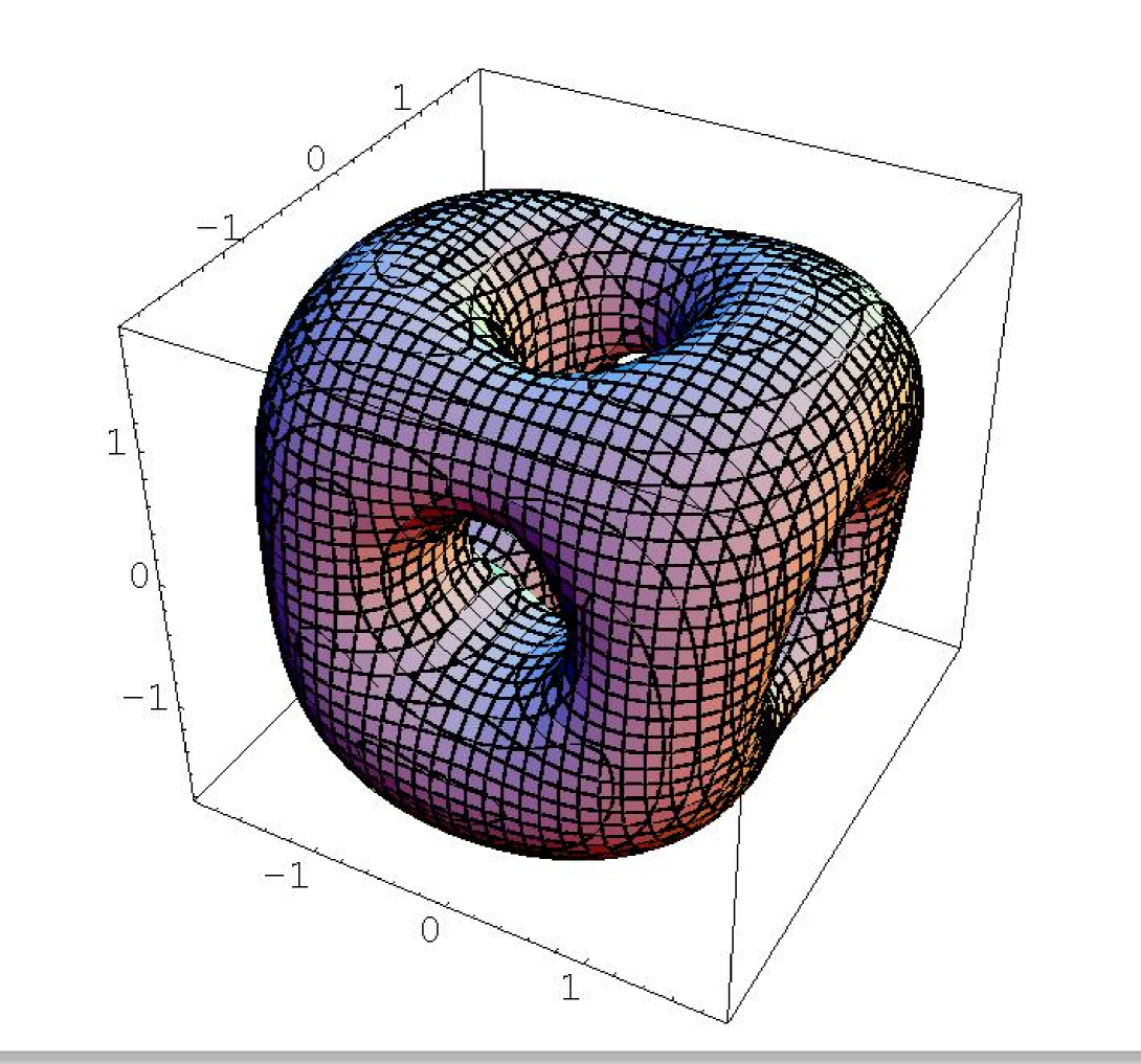
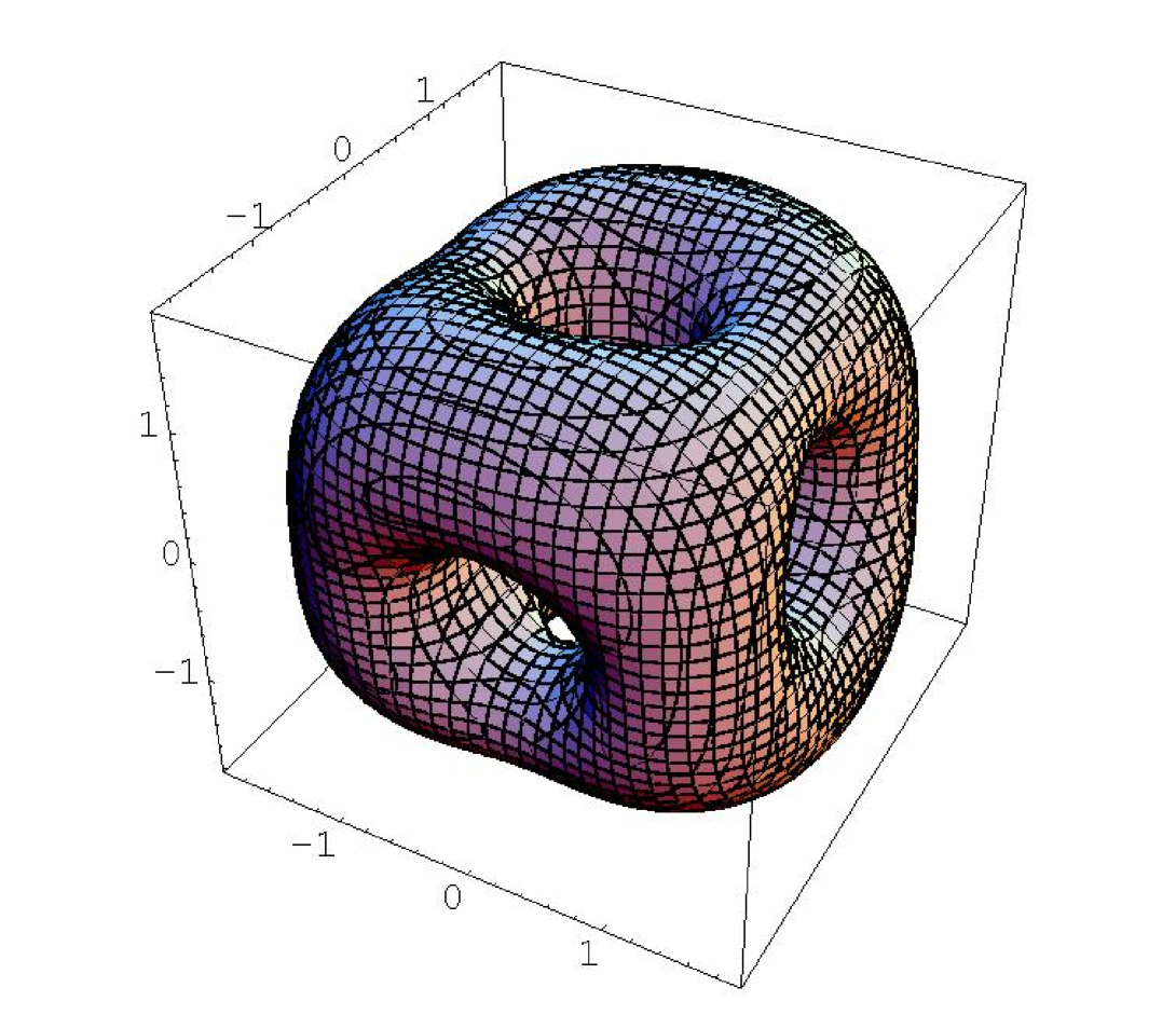
Figure 2: $B=4$, $R_{th,z}(\xi)$: (Left) $\epsilon>0$; (Right) $\epsilon<0$.

The last triplet mode corresponds to the pinching and stretching of two opposite edges of the cube so that two of the opposite faces of the cube are deformed into a rhombus.

$$R_{rhomb,x}(\xi) = \frac{P_{0}+(\frac{1}{2}+\frac{\sqrt{3}\,i}{2})\,\epsilon\,\xi^{3}+(\frac{1}{2}+\frac{\sqrt{3}\,i}{2})\,\epsilon\,\xi}{Q_{0}-(\frac{1}{2}-\frac{\sqrt{3}\,i}{2})\epsilon\,\xi^{3}-(\frac{1}{2}-\frac{\sqrt{3}\,i}{2})\,\epsilon\,\xi},$$

$$R_{rhomb,y}(\xi) = \frac{P_{0}+(\frac{\sqrt{3}}{2}+\frac{i}{2})\,\epsilon\,\xi^{3}-(\frac{\sqrt{3}}{2}+\frac{i}{2})\,\epsilon\,\xi}{Q_{0}+(\frac{\sqrt{3}}{2}-\frac{i}{2})\epsilon\,\xi^{3}-(\frac{\sqrt{3}}{2}-\frac{i}{2})\,\epsilon\,\xi},$$

$$R_{rhomb,z}(\xi) = \frac{P_{0}-\sqrt{3}\,i\,\epsilon\,\xi^{2}-\epsilon}{Q_{0}-\epsilon\,\xi^{4}+\sqrt{3}\,i\,\epsilon\,\xi^{2}}.$$ (51)

The energy density plots are presented in figure 3. The eigen value of the rhombus mode is $\omega_{rhomb}=0.7395$ for $m_{\pi}=0$ and $\omega_{rhomb}=0.9113$ for $m_{\pi}=0.526$.

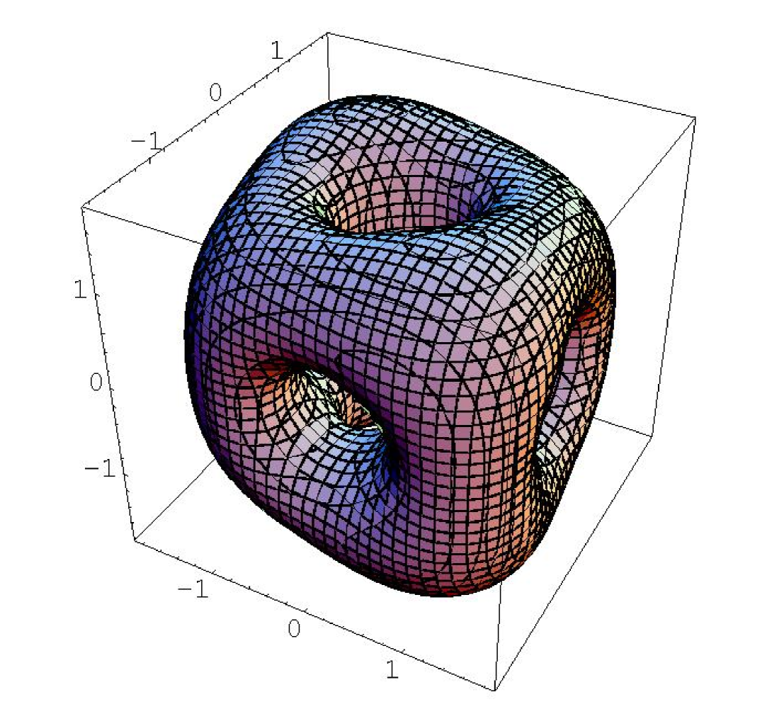
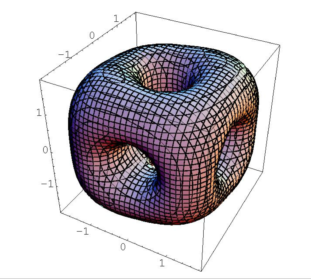
Figure 3: $B=4$, $R_{rhomb,z}(\xi)$: (Left) $\epsilon>0$; (Right) $\epsilon<0$.

The doublet mode

$$R_{scat1}(\xi) = \displaystyle\frac{P_{0}-2\sqrt{3}\,\epsilon\,\xi^{2}}{Q_{0}+i\,\epsilon\,\xi^{4}+i\,\epsilon},$$

$$R_{scat2}(\xi) = \displaystyle\frac{P_{0}+i\,\epsilon\,\xi^{2}}{Q_{0}-i\,\epsilon\,\xi^{2}},$$ (52)

corresponds to a deformation where the cube is alternatively stretched and then flattened along one of the symmetry axis going through the center of the cube’s faces. A combination of a stretch along two of the (perpendicular) axis is equivalent to a stretch along the third axis. This corresponds to the scattering mode of two tori along their axis of symmetry as shown in figure 4. The eigen value for this class of modes is $\omega_{str}=0.818$ for $m_{\pi}=0$ and $\omega_{str}=1.0064$ for $m_{\pi}=0.526$.

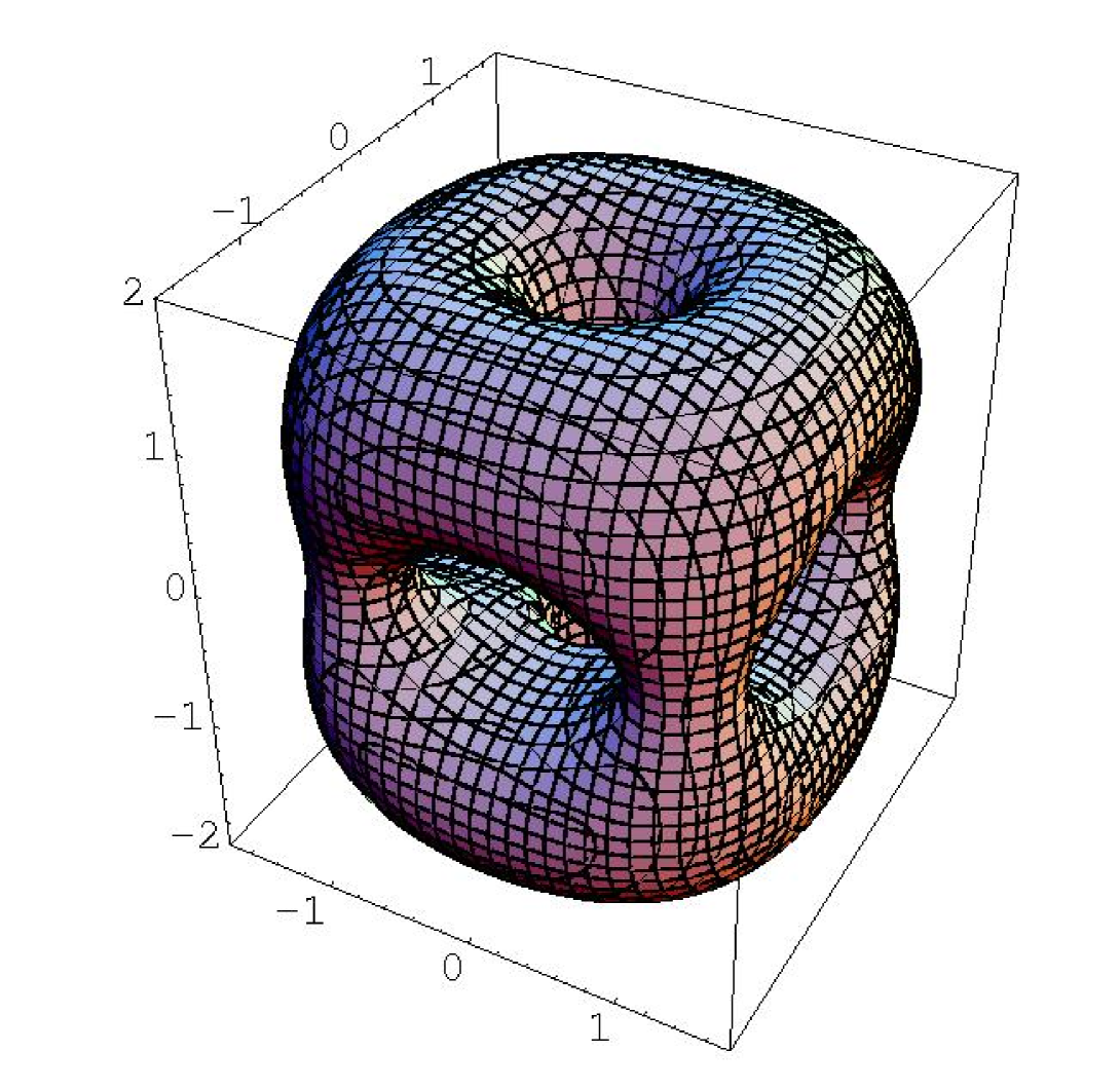
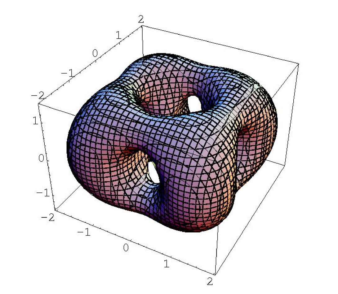
Figure 4: $B=4$, $R_{scat2}(\xi)$: (Left) $\epsilon>0$; (Right) $\epsilon<0$.

The singlet mode

$$R_{tet} = \frac{P_{0}}{Q_{0}(1-\epsilon)}$$ (53)

corresponds to a tetrahedral deformation of the cube as illustrated in Figure 5. Its eigen value is $\omega_{tet}=1.1355$ for $m_{\pi}=0$ and $\omega_{tet}=1.4026$ for $m_{\pi}=0.526$.

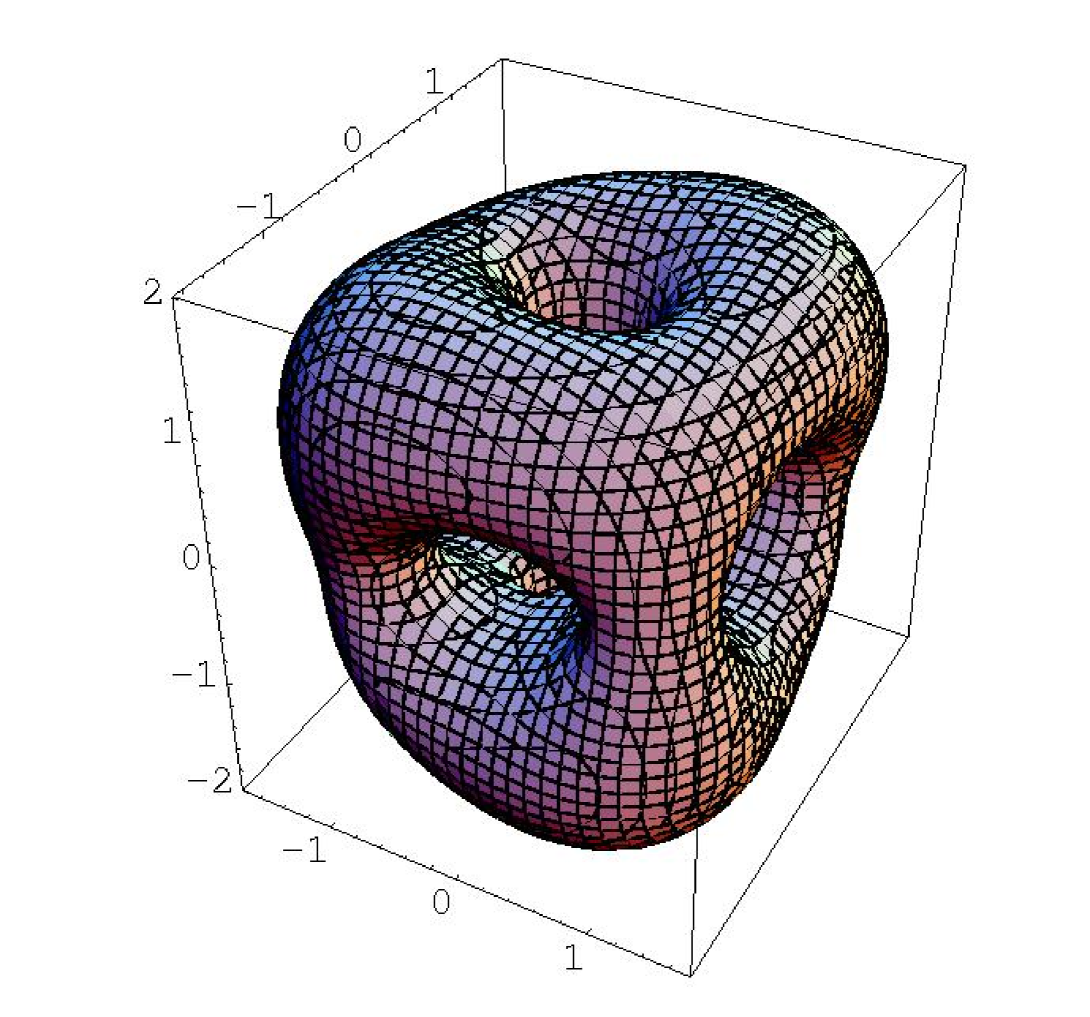
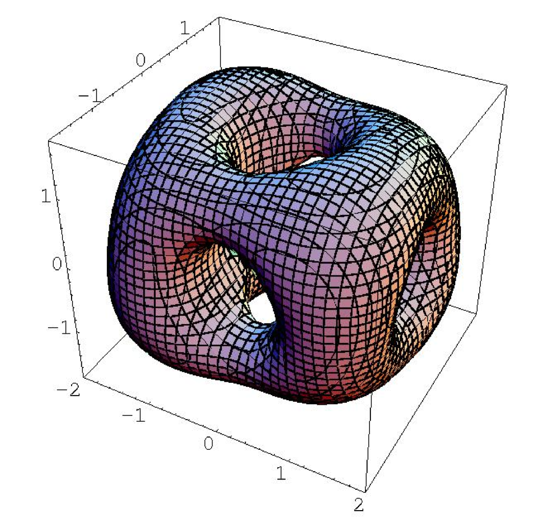
Figure 5: $B=4$, $R_{tet}(\xi)$: (Left) $\epsilon>0$; (Right) $\epsilon<0$.

4 Radial Vibrations

The Euler-Lagrange equation for the radial perturbation $g$ can be easily derived from (34):

$$(\ddot{g}-g^{\prime\prime})\,\Bigl{(}2\mathcal{B}\sin^{2}f_{0}+r^{2}\Bigr{)}-\Bigl{(}2r+2\mathcal{B}f^{\prime}_{0}\sin(2f_{0})\Bigl{)}\,g^{\prime}-\Bigl{(}-2\mathcal{B}\cos(2f_{0})+2\mathcal{B}f^{\prime 2}_{0}\cos(2f_{0})$$

$$+2\mathcal{B}f^{\prime\prime}_{0}\sin(2f_{0})-\frac{\mathcal{I}_{0}}{r^{2}}\Big{[}6(\sin^{2}f_{0})\,(\cos^{2}f_{0})-2\sin^{4}f_{0}\Big{]}-m^{2}r^{2}\cos(pf_{0})\Bigr{)}\,g\;=0,$$ (54)

where $g^{\prime}=\frac{\partial}{\partial r}$ and $\dot{g}=\frac{\partial}{\partial t}$. Taking a perturbation of the form

$$g(r,t)=g_{0}(r)\,\sin(\omega t)$$ (55)

and inserting it into (54) leads to a Sturm-Liouville equation where $\omega^{2}$ is the eigen value.

Notice that when $\omega>m$, any perturbation is radiated away and there are no genuine vibration modes. When the pion mass $m_{\pi}$ is too small, there are thus no genuine radial vibration modes. On the other hand, the Skyrmion still has so-called pseudo-vibration modes, as studied by Bizon et al.[8], where the excitation energy is radiated away relatively slowly. In a quantum theory these modes would correspond to resonances.

We have solved (54) numerically for several baryon numbers and several values of the pion mass and the parameter $p$. Our results are summarised in figure 6 where we present the vibration frequency $\omega$ as a function of the pion mass for different baryon number values.

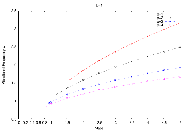
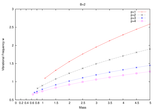
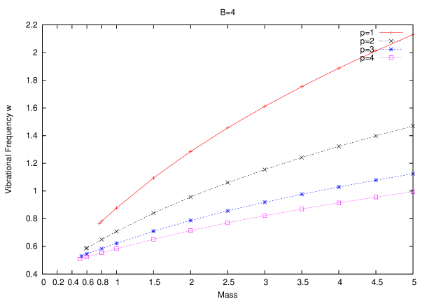
Figure 6: Radial Vibration frequency for $\mathcal{B}$=1$,\mathcal{B}$=2, $\mathcal{B}$=4.

On table 3 we present the critical value of the pion mass below which there is no genuine vibration mode. Notice that the case $B=1$ is the exact hedgehog solution and corresponds to a single nucleon. The critical value of the mass for that case, can thus be interpreted as an upper bound for the pion mass when it is taken as an adjustable parameters [9][10], as the proton has no stable excited state.

$B$ $\setminus$ p	1	2	3	4
1	1.60	1.19	0.96	0.85
2	1.10	0.82	0.71	0.65
4	0.77	0.59	0.53	0.51
6	0.60	0.47	0.44	0.43
7	0.56	0.44	0.42	0.41
9	0.47	0.38	0.36	0.36
17	0.33	0.28	0.27	0.27

Table 3: Critical Mass as a function of $B$ and $p$.

5 Comparison

Several years ago, Barnes et al[5][6] computed the vibration modes of the $B=2$ and $B=4$ Skyrmion solutions numerically. In their work, they only considered the standard mass term, $p=1$ and the pion mass that they used, in our parametrisation is given by $m_{\pi}=0.526$. By comparing their results with ours, we will be able to asses the quality of the rational map for the estimation of the vibration modes.

The method used by Barnes et al. consists in solving numerically small fluctuations of the Skyrme field around a static solution obtained numerically too. To solve the Skyrme equation numerically, one has to invert a matrix that is field-dependant. To improve the efficiency of their code, and motivated by the fact that they only studied small vibrations, Barnes et al. set that matrix to the one obtained from the stationary field. This effectively pinned the position and iso-orientation of the Skyrmion, thus breaking the translation and iso-rotation zero modes. On the other hand, the rotations symmetry was preserved, apart from the symmetry breaking introduced by the square lattice and the periodic boundary conditions.

We compare our results with those of [5] and [6] in Tables 4 and 5. One can identify the various vibration modes by comparing the dimension of the subspace they span, i.e. the dimension of the representation they belong to, as well as their symmetries and the deformation induced in energy density plots. Figures 2 in [5] match exactly those we have obtained for the vibrational modes of the rational map of $B=4$. Figure 3 in [6], once translated to what is plotted in figure 1, also matches our observation for $B=2$.

For $B=2$, we had to read the values of $\omega$ from figure 1 in [6]. There is only one genuine vibration mode, the so-called scattering mode. The frequency obtained from the rational map for that mode is much higher than the one obtained numerically, but the frequency obtained from Barnes et al. indicates that it is a genuine vibration mode.

The mode described as a dipole breathing motion in [6], turns out to be a broken translation. Notice also that the breathing mode is a pseudo vibration mode for both the numerical and the rational map results. The radiative modes observed in [6] are the results of the numerical method used and are excluded from the rational map ansatz, except from the mode with symmetry $A_{1u}$ which happens to be a broken translation mode.

For $B=4$, the modes that we obtained match those obtained in [5]. The mode with $\omega_{num}=0.655$ in [5] turns out to be a broken translation mode rather than a proper vibration mode. This is supported by comparing the energy densities for that mode, not presented in this paper, and the one given in [5], as well as the symmetry of that mode. Apart from that, the rational map ansatz predicts 5 non-null vibration modes out of 6 (the diagonal mode, with $\omega_{num}=0.738$, is missing). Symmetry considerations suggest that the radiative mode with $\omega_{num}=0.587$ might be a pseudo-iso-rotational mode, but it is difficult to be conclusive as one would need to know more about this numerical mode to make a definite statement. If the vibration modes obtained from the rational map ansatz match the one obtained numerically rather well, the predictions for the frequencies of these modes are rather poor and are not even in the correct order. Overall, the rational map ansatz appears to be stiffer than real Skyrmion solutions.

		Numerical[6]			Ansatz
$\omega$	Degeneracy	Description	Symmetry	$\omega$	Degeneracy	Description	Symmetry
0.03	2	broken rotational modes	$E_{1g}$	0	3	$x$, $y$ rotational modes $(R_{rot,x},R_{rot,y})$	$E_{1g}+A_{2g}$
		(around $x$ and $y$ axes)				and $z$ (iso)rotational mode $(R_{rot,z})$
0.31	2	2 Skyrmions scattering mode	$E_{2g}$	1.225536	2	2 Skyrmions scattering mode $(R_{s1},R_{s2})$	$E_{2g}$
0.49	1	radiative mode	$A_{1u}$
				0.583500	1	broken $z$ translation $(R_{btr,z})$	$A_{1u}$
0.52	2	radiative mode	$E_{2g}$
0.75	1	breathing mode	$A_{1g}$	0.76	1	breathing mode	$(A_{1g})$
0.84	2	a dipole ‘breathing’ motion$\dagger$	$E_{1u}$	0.846727	2	broken $x$, $y$ translation $(R_{btr,x},R_{btr,y})$	$E_{1u}$

Table 4: Comparison of vibrational frequency between the numerical results and the rational map ansatz, $B=2$.

• Its description of the energy density matches that of the broken $x$, $y$ translational zero mode obtained from the rational map ansatz; however, this representation, $E_{1u}$, coincides with the doublet of $x$, $y$ translational zero mode of the 2-monopole toroidal BPS solution.

		Numerical[5]				Ansatz
$\omega$	Degeneracy	Description	Symmetry	$\omega$	Degeneracy	Description
				0	2	iso-rotation $(R_{iso,x},R_{iso,y})$	$E_{u}$	$E^{O}$	2
0.070	3	broken rotation	$F_{1g}$	0	3	rotation $(R_{rot,x},R_{rot,y},R_{rot,z})$
0.367	2	deuteron scattering mode	$E_{g}$	1.006370	2	deuteron scattering mode $(R_{scat1},R_{scat2})$
0.405	1	tetrahedral mode	$A_{2u}$	1.402608	1	tetrahedral mode $(R_{tet})$
0.419	3	rhombus mode	$F_{2g}$	0.911260	3	rhombus mode $(R_{rhomb,x},R_{rhomb,y},R_{rhomb,z})$
0.513	3	4 Skyrmions mode	$F_{2u}$	0.750841	3	4 Skyrmions mode $(R_{tb,x},R_{tb,y},R_{tb,z})$
0.545	2	radiative mode	$E_{g}$
				0	1	iso-rotation $(R_{iso,z})$
0.587	1	radiative mode	$A_{2u}$
0.605	1	breathing mode	$A_{1g}$	0.64	1	breathing mode
0.655	3	broken translation	$F_{1u}$	0.562538	3	broken translation $(R_{btr,x},R_{btr,y},R_{btr,z})$
0.738	3	diagonal mode	$F_{2g}$
0.908	3	lowest nonzero radiative mode

Table 5: Comparison of vibrational frequency between the numerical result and the rational map ansatz, $B=4$.

• Its description of the energy density matches that of the broken $x$, $y$ translational zero mode obtained from the rational map ansatz; however, this representation, $E_{1u}$, coincides with the doublet of $x$, $y$ translational zero mode of the 2-monopole toroidal BPS solution.

6 Conclusion

The rational map ansatz has been shown to be a good approximation to the shell-like solutions of the Skyrme model, i.e. when the pion mass is null or relatively small, or when the baryon number is small. In this paper we have shown that the rational map ansatz can also be used to study the vibration modes of the Skyrmion solutions and that qualitatively it produces the correct vibration modes. For $B=1$, for which the ansatz is actually the exact solution, and $B=2$, the vibration modes are all predicted, but for $B=4$ they are all predicted except for one, the one with the largest vibration frequencies.

On the other hand, the vibration frequencies obtained from the rational map ansatz are quite poor when compared to the frequencies obtained numerically in [5] and [6]. The relative order is not even correct. We interpret this result by saying that the rational map ansatz is too stiff and that the configuration is restrained to vibrate in a subspace that is too narrow.

Our study has also shown that some of the modes observed by Barnes et al. were mistakenly taken as genuine vibration modes when they are actually broken vibration modes.

Acknowledgement

We would like to thanks P. Sutcliffe for useful discussions and comments.

References

- [1] T.H.R. Skyrme, Proc. Roy. Soc. Lond., A260, 127-138 (1961).
- [2] E. Witten, Nucl. Phys. B223, 422 (1983), E. Witten, Nucl. Phys. B223, 433 (1983)
- [3] R.A. Battye and P.M. Sutcliffe, Rev. Math. Phys. 14, 29 (2002)
- [4] C.J. Houghton, N.S. Manton and P.M. Sutcliffe, Nucl. Phys. B 510, 507 (1998).
- [5] C. Barnes, K. Baskerville and N. Turok, Phys. Rev. Lett. 79: 367 (1997).
- [6] C. Barnes, K. Baskerville and N. Turok, Phys. Rev. B 441: 180 (1997).
- [7] V.B. Kopeliovich, B. Piette and W.J. Zakrzewski, Phys. Rev. D 73, 014006 (2006)
- [8] P. Bizon, T. Chmaj and A. Rostworowski, Phys. Rev. D 75, 121702 (2007)
- [9] R.A. Battye, S. Krush and P.M. Sutcliffe, Phys. Lett. B 626, 120 (2005)
- [10] R.A. Battye, N. Manton and P.M. Sutcliffe, Proc. R. Soc. 463, 261 (2007)