Hyperbolic graphs of small complexity

Abstract.

In this paper we enumerate and classify the “simplest” pairs $(M,G)$ where $M$ is a closed orientable $3$-manifold and $G$ is a trivalent graph embedded in $M$.

To enumerate the pairs we use a variation of Matveev’s definition of complexity for $3$-manifolds, and we consider only $(0,1,2)$-irreducible pairs, namely pairs $(M,G)$ such that any 2-sphere in $M$ intersecting $G$ transversely in at most $2$ points bounds a ball in $M$ either disjoint from $G$ or intersecting $G$ in an unknotted arc. To classify the pairs our main tools are geometric invariants defined using hyperbolic geometry. In most cases, the graph complement admits a unique hyperbolic structure with parabolic meridians; this structure was computed and studied using Heard’s program Orb and Goodman’s program Snap.

We determine all $(0,1,2)$-irreducible pairs up to complexity 5, allowing disconnected graphs but forbidding components without vertices in complexity 5. The result is a list of 129 pairs, of which 123 are hyperbolic with parabolic meridians. For these pairs we give detailed information on hyperbolic invariants including volumes, symmetry groups and arithmetic invariants. Pictures of all hyperbolic graphs up to complexity 4 are provided. We also include a partial analysis of knots and links.

The theoretical framework underlying the paper is twofold, being based on Matveev’s theory of spines and on Thurston’s idea (later developed by several authors) of constructing hyperbolic structures via triangulations. Many of our results were obtained (or suggested) by computer investigations.

1. Introduction

The study of knotted graphs in $3$-manifolds is a natural generalization of classical knot theory, with potential applications to chemistry and biology (see e.g. [10]). In knot theory, extensive knot tables have been built up through the work of many mathematicians (see e.g. Conway [6] and Hoste–Thistlethwaite–Weeks [21]). There has been much less work on the tabulation of knotted graphs, but some knotted graphs in $S^{3}$ have been enumerated in order of crossing number by Simon [45], Litherland [27], Moriuchi [38, 39], and Chiodo et. al. [5].

In this paper we classify the simplest trivalent graphs in general closed $3$-manifolds. We first enumerate them using a notion of complexity which extends Matveev’s definition for $3$-manifolds [32], and then we classify them with the help of geometric invariants, mostly defined using hyperbolic geometry.

More precisely, the objects considered in this paper are pairs $(M,G)$ where $M$ is a closed, connected orientable $3$-manifold and $G$ is a trivalent graph in $M$. The graph $G$ may contain loops and multiple edges, and is possibly disconnected (in particular, $G$ can be a knot or a link). To avoid “wild” embeddings we work in the piecewise linear category: thus $M$ is a PL-manifold and $G$ is a 1-dimensional subcomplex, and we aim to classify graphs up to PL-homeomorphisms of pairs.

Following [32], a compact polyhedron $P$ is called simple if the link of every point of $P$ embeds in the 1-skeleton of the tetrahedron (the complete graph with 4 vertices). Points having the whole of this graph as a link are called vertices of $P$. Moreover, as defined in [41], $P$ is a spine of a pair $(M,G)$ if it embeds in $M$ so that its complement is a finite union of balls intersecting $G$ in the simplest possible ways, as shown in Figure 1.

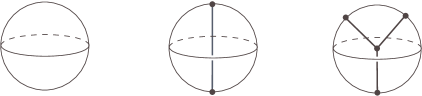
Figure 1. Balls in the complement of a spine.

As usual in complexity theory, the complexity $c(M,G)$ is then defined as the minimal number of vertices in a simple spine of $(M,G)$. The case considered in [41] is actually that of 3-orbifolds, but the definition of complexity is the same as just given, except that a contribution of the edge labels is also introduced. When $G=\emptyset$ we recover the original definition of Matveev, thus getting the equality $c(M)=c(M,\emptyset)$. In general, we have $c(M)\leqslant c(M,G)$.

For manifolds, Matveev showed that complexity is additive under connected sum and that it behaves particularly well on irreducible manifolds (i.e. manifolds in which every 2-sphere bounds a 3-ball). In particular, there exist only finitely many irreducible manifolds with given complexity. These facts extend to the context of the pairs $(M,G)$ described above, with the following notion of irreducibility: $(M,G)$ is $(0,1,2)$-irreducible if every 2-sphere embedded in $M$ and meeting $G$ transversely in at most two points bounds a ball intersecting $G$ as in Figure 1, left or centre (in particular, there exists no 2-sphere meeting $G$ in one point).

This paper is devoted to the enumeration and the geometric investigation of all $(0,1,2)$-irreducible graphs $(M,G)$ of small complexity. As usual in $3$-dimensional topology, a key role in the study of our graphs is played by invariants coming from hyperbolic geometry, which in particular provided the tools we used in most cases to distinguish the pairs from each other.

While the complement of $G$ in $M$ very often has no hyperbolic structure with geodesic boundary (for instance, it is often a handlebody), most pairs $(M,G)$ are indeed hyperbolic in a more general sense, namely they are hyperbolic with parabolic meridians. This means that $M\setminus G$ carries a metric of constant sectional curvature $-1$ which completes to a manifold with non-compact geodesic boundary having:

• toric cusps at the knot components of $G$,

• annular cusps at the meridians of the edges of $G$, and

• geodesic 3-punctured boundary spheres at the vertices of $G$.

This hyperbolic structure is the natural analogue of the complete hyperbolic structure on a knot or link complement and is also useful when studying orbifold structures on $(M,G)$.

By Mostow-Prasad rigidity, a hyperbolic structure with parabolic meridians is unique if it exists, so its geometric invariants only depend on $(M,G)$. One can therefore use the volume and Kojima’s canonical decomposition [24, 25] to distinguish hyperbolic graphs. For the pairs in our list we have constructed and analyzed the hyperbolic structure using the computer program Orb, written by the first named author [19].

Since knots and links have already been widely studied in many contexts, this paper focuses mostly on graphs containing vertices.

Number of hyperbolic graphs

Table 1 gives a summary of our results. Up to complexity $4$ our census of hyperbolic graphs $(M,G)$ is complete and contains $45$ elements, consisting of 5 knots, 24 $\theta$-graphs, 13 handcuffs, and 3 distinct connected graphs with four vertices. The graph types occurring are shown in Figure 2. In complexity 5 we decided to rule out knot components, and we found 78 more hyperbolic graphs. Out of our 123 graphs, 36 lie in $S^{3}$.

type	$c=1$	$c=2$	$c=3$	$c=4$	$c=5$
knot (in $S^{3}$)	0 (0)	0 (0)	1 (1)	4 (1)	– (–)
$2t$ (in $S^{3}$)	0 (0)	2 (1)	4 (1)	18 (4)	49 (10)
$2h$ (in $S^{3}$)	1 (1)	1 (0)	3 (2)	8 (2)	27 (8)
$4a$ (in $S^{3}$)	0 (0)	1 (1)	0 (0)	0 (0)	2 (2)
$4b$ (in $S^{3}$)	0 (0)	0 (0)	0 (0)	1 (1)	0 (0)
$4c$ (in $S^{3}$)	0 (0)	0 (0)	0 (0)	1 (1)	0 (0)

Table 1. Numbers of hyperbolic graphs. When $c=5$ we have not investigated graphs having knot components. The other graph types not mentioned were all investigated and found to have no representative.

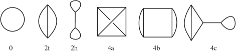
Figure 2. Names of abstract graph types.

Detailed information on all the 123 hyperbolic graphs up to complexity 5, including the volume and a description of the canonical decomposition, will be given in Section 5, while pictures of graphs up to complexity 4 will be shown in Section 7.

Complexity and volume

As shown in Table 1, there is a single hyperbolic graph of smallest complexity $c=1$. It is a handcuff graph in $S^{3}$, described in Figure 4 and Example 2.1. It is also the hyperbolic graph with vertices of least volume 3.663862377… This fact confirms the following relationships between complexity and hyperbolic geometry, which have already been verified for closed manifolds [32, 15], cusped manifolds [2, 3, 14, 15], and manifolds with arbitrary (geodesic) boundary [13, 26, 36, 11]:

1. Objects having complexity zero are not hyperbolic.

2. Among hyperbolic ones, the objects having lowest volume have the lowest complexity.

Note that complexity and volume may share the same first segments of hyperbolic objects (as they do) but are qualitatively different globally, because in general there are finitely many hyperbolic objects of bounded complexity, while infinitely many ones may have bounded volume thanks to Dehn surgery.

Compact totally geodesic boundary

It may happen that $M\setminus G$ has a hyperbolic metric which completes to a manifold with compact totally geodesic boundary. In this case we say that $(M,G)$ is hyperbolic with geodesic boundary, which implies that $(M,G)$ is also hyperbolic (with parabolic meridians), but as mentioned above the converse is often false. By analyzing the graphs in Table 1, we have established the following:

Proposition 1.1.

Up to complexity $5$ there exist $3$ graphs $(M,G)$ which are hyperbolic with geodesic boundary, shown in Figure 3. They all belong to the set of $8$ minimal-volume such manifolds described by Kojima–Miyamoto [26] and Fujii [13], and they include Thurston’s knotted $Y$ [48].

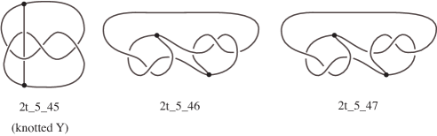
Figure 3. Graphs whose complements admit a hyperbolic structure with geodesic boundary.

Non-hyperbolic graphs

The (0,1,2)-irreducible graphs of complexity 0 were detected by theoretical means, see Section 3. There are 3 knots (cores of Heegaard tori in $S^{3}$, $L(3,1)$ and ${\mathbb{P}}^{3}$) and the trivial $\theta$-graph in $S^{3}$, and they are all non-hyperbolic. In complexity $c=1,2$ we have classified all (0,1,2)-irreducible non-hyperbolic graphs, finding only 16 knots and two links. The same phenomenon happens for $c=3,4$, where we have shown that only knots and links are (0,1,2)-irreducible and non-hyperbolic. However we refrained from classifying them completely, confining ourselves to those in $S^{3}$ with $c=3$. Since our primary interest was in hyperbolic graphs, we decided to rule out knot components in complexity $5$, but quite interestingly we have found some non-hyperbolic examples in this case. Our results are summarized by Table 2 and the next statement:

Proposition 1.2.

The only $(0,1,2)$-irreducible non-hyperbolic graphs $(M,G)$ with $c(M,G)\leqslant 5$ such that $G$ has no knot component are the trivial $\theta$-graph in $S^{3}$, which has complexity $0$, and five pairs in complexity $5$, where $G$ is a $\theta$-graph and $M\setminus G$ contains an embedded Klein bottle.

type	$c=0$	$c=1$	$c=2$	$c=3$	$c=4$	$c=5$
knot (in $S^{3}$)	3 (1)	4 (1)	12 (1)	– (4)	– (–)	– (–)
2-link (in $S^{3}$)	0 (0)	1 (1)	1 (0)	– (1)	– (–)	– (–)
2t (in $S^{3}$)	1 (1)	0 (0)	0 (0)	0 (0)	0 (0)	5 (0)

Table 2. Numbers of (0,1,2)-irreducible non-hyperbolic graphs. When $c=5$ we have not investigated graphs having knot components; – indicates that graphs of this type were not classified. The graph types not mentioned were all investigated and found to have no representative.

A precise description of the knots, links and graphs appearing in Table 2 will be provided in Section 6.

Some open problems

We conclude this introduction by suggesting a few problems for further investigation.

1. Enumerate the first few hyperbolic graphs with parabolic meridians in order of increasing hyperbolic volume.

2. Enumerate the first few hyperbolic $3$-manifolds of finite volume with (compact or non-compact) geodesic boundary in order of increasing hyperbolic volume.

3. Enumerate the first few closed hyperbolic 3-orbifolds in order of increasing complexity as defined in [41].

4. Enumerate the first few closed hyperbolic 3-orbifolds in order of increasing hyperbolic volume.

5. Determine the exact complexity of infinite families of knotted graphs, for example the torus knots in lens spaces (see Conjecture 6.4 below).

Note that Kojima and Miyamoto [26, 36] have already identified the lowest volume hyperbolic $3$-manifolds with compact and non-compact geodesic boundary. Perhaps the “Mom technology” introduced by Gabai, Meyerhoff and Milley [14, 15] may offer an approach to (1) and (2). Recent work of Martin with Gehring and Marshall [16, 29] has identified the lowest volume orientable hyperbolic 3-orbifold.

2. Hyperbolic geometry

In this section we review the main geometric notions and results we will need in the rest of the paper.

2.1. Hyperbolic structures with parabolic meridians

To help classify knotted graphs, we will study hyperbolic structures analogous to the compete hyperbolic structure on the complement of a knot or link. Given a graph $G$ in a closed orientable $3$-manifold $M$, let $N$ be the manifold obtained from $M\setminus G$ by removing an open regular neighbourhood of the vertex set of $G$. Thus $N$ is a non-compact $3$-manifold with boundary consisting of 3-punctured spheres, one corresponding to each vertex of $G$. Then we say that $(M,G)$ has a hyperbolic structure with parabolic meridians if $N$ admits a complete hyperbolic metric of finite volume with geodesic boundary (with toric and annular cusps). Equivalently, the double $D(N)$ of $N$ admits a complete hyperbolic metric of finite volume (with toric cusps). Such a hyperbolic structure on $N$ is unique by a standard argument using Mostow-Prasad rigidity [46] and Tollefson’s classification [49] of involutions with 2-dimensional fixed point set (see [47] and also [12]).

Example 2.1.

The simplest hyperbolic handcuff graph $(S^{3},G)$ can be obtained from one tetrahedron with the two front faces folded together and the two back faces folded together giving a triangulation of $S^{3}$ with the graph $G$ contained in the 1-skeleton as shown in Figure 4.

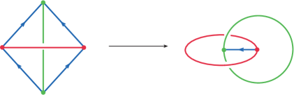
Figure 4. The simplest hyperbolic handcuff graph.

If we truncate the vertices of the tetrahedron until all edge lengths are zero, the result can be realized geometrically by a regular ideal octahedron in hyperbolic space, as shown in Figure 5. We can then glue the 4 unshaded faces together in pairs so that the other 4 shaded faces form two totally geodesic 3-punctured spheres.

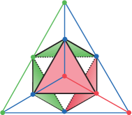
Figure 5. Truncating the vertices of a tetrahedron produces a regular ideal octahedron whose unshaded faces can be glued in pairs to give a hyperbolic structure with parabolic meridians on the graph of Figure 4.

This gives a hyperbolic structure with parabolic meridians for $(S^{3},G)$ with hyperbolic volume 3.663862377… The work of Miyamoto and Kojima [26, 36] shows that this is the smallest volume for trivalent graphs. Their work also implies that a trivalent graph having this volume is obtained by identifying the unshaded faces of an ideal octahedron as above, and hence has complexity $1$. Therefore the handcuff graph in Figure 4 is the unique graph of minimal volume.

We next describe topological conditions for the existence of a hyperbolic structure with parabolic meridians. Let $X$ denote the graph exterior, i.e., the compact manifold obtained from $M$ by removing an open regular neighbourhood of the graph $G$. Then ${\partial}X$ is a disjoint union of pairs of pants (corresponding to the vertices of $G$) and a collection of annuli and tori $P\subset X$ (corresponding to the edges and knots in $G$). Thurston’s hyperbolization theorem for pared $3$-manifolds [37, 23] implies the following:

Theorem 2.2.

$(M,G)$ admits a hyperbolic structure with parabolic meridians if and only if

• $X$ is irreducible and homotopically atoroidal,

• $P$ consists of incompressible annuli and tori,

• there is no essential annulus $(A,{\partial}A)\subset(X,P)$, and

• $(X,P)$ is not a product $(S,{\partial}S)\times[0,1]$ where $S$ is a pair of pants.

This hyperbolic structure is unique up to isometry.

Remark 2.3.

To obtain a hyperbolic structure with geodesic boundary on a general pared manifold $(X,P)$, we would need to add the requirements that ${\partial}X\setminus P$ incompressible and $(X,P)$ is acylindrical (i.e., every annulus $(A,{\partial}A)\subset(X,{\partial}X\setminus P)$ is homotopic into ${\partial}X$). But these conditions follow here since ${\partial}X\setminus P$ consists of $3$-punctured spheres (see [1, pp. 243-244]).

The conditions for hyperbolicity simplify considerably when $(M,G)$ is $(0,1,2)$-irreducible, as defined in the introduction. To elucidate the notion, we say that $(M,G)$ is:

• 0-irreducible if every 2-sphere in $M$ disjoint from $G$ bounds a 3-ball in $M$ disjoint from $G$;

• 1-irreducible if there exists no 2-sphere in $M$ meeting $G$ transversely in a single point;

• 2-irreducible if every 2-sphere in $M$ meeting $G$ transversely in two points bounds a ball in $M$ that intersects $G$ in a single unknotted arc.

Then a graph is $(0,1,2)$-irreducible if it is $i$-irreducible for $i=0,1,2$.

Theorem 2.4.

$(M,G)$ admits a hyperbolic structure with parabolic meridians if and only if

• $(M,G)$ is $(0,1,2)$-irreducible,

• $X$ is homotopically atoroidal and is not a solid torus or the product of a torus with an interval, and

• $(M,G)$ is not the trivial $\theta$-graph in $S^{3}$.

Proof.

It is easy to check that the conditions listed are necessary for hyperbolicity. To show that they are sufficient, first note that $0$-irreducibility of $(M,G)$ implies that $X$ is irreducible, and $1$-irreducibility implies that $P$ is incompressible or $X$ is a solid torus, but the latter possibility is excluded. Moreover $(X,P)$ is not a product $(S,\partial S)\times[0,1]$ where $S$ is a pair of pants, because $(M,G)$ is not the trivial $\theta$-graph in $S^{3}$. According to the previous theorem we are only left to show that there cannot exist an essential annulus $(A,{\partial}A)\subset(X,P)$. Suppose the contrary and note that each of the two components of $\partial A$ is incident to either an annular or a toric component of $P$. We show that the existence of such an annulus $A$ is impossible by considering the three possibilities:

1. If $A$ is only incident to annuli of $P$, we readily see that $2$-irreduciblity is violated.

2. If $A$ is incident to an annular component $A^{\prime}$ of $P$ and a torus component $T$ of $P$, then the boundary of a regular neighbourhood of $A\cup T$ is another annulus incident to $A^{\prime}$ only. Again we see that $2$-irreducibility is violated, since the resulting sphere does not bound a ball containing a single unknotted arc.

3. If $A$ is incident to toric components only, proceeding as in the previous case we find one or two tori, depending on whether the toric components are distinct or not. Homotopic atoroidality implies that these tori must be compressible or boundary parallel in $X$. Using irreducibility of $X$ and incompressibility of $A$, we find that $X$ is Seifert fibred with the core circle of $A$ as a fibre and base space either a pair of pants, an annulus with at most one singular point, or a disc with at most two singular points. By homotopic atoroidality, we deduce that $X$ is the product of a torus and an interval or a solid torus, contrary to our assumptions.

∎

Corollary 2.5.

If $G$ is a trivalent graph containing at least one vertex, then $(M,G)$ is hyperbolic with parabolic meridians if and only if $(M,G)$ is $(0,1,2)$-irreducible, geometrically atoroidal and not the trivial $\theta$-graph in $S^{3}$.

2.2. Hyperbolic structures with geodesic boundary

Let $(M,G)$ be a graph, and let $X$ denote the graph exterior as above. Let us define $Y$ as the manifold obtained by mirroring $X$ in its non-toric boundary components, so $Y$ is either closed or bounded by tori. Then $X$ minus its toric boundary components has a hyperbolic structure with totally geodesic boundary if and only if the interior of $Y$ has a complete hyperbolic structure. By Thurston’s hyperbolization theorem [37, 23] and Mostow-Prasad rigidity (see [47, p. 14]) we then have:

Theorem 2.6.

$X$ minus its toric boundary components admits a hyperbolic structure with totally geodesic boundary if and only if $X$ is irreducible, boundary incompressible, homotopically atoroidal, and acylindrical. This hyperbolic structure is unique up to isometry.

Comparing Theorems 2.2 and 2.6 one easily sees that if $X$ minus its toric boundary components admits a hyperbolic structure with geodesic boundary, then $(M,G)$ admits a hyperbolic structure with parabolic meridians. The converse is however false, as most of the pairs $(M,G)$ described below show.

2.3. Hyperbolic orbifolds

One of the initial motivations of our work was the study of hyperbolic $3$-orbifolds, but the analysis of graphs turned out to be interesting enough by itself, so we decided to leave orbifolds for the future. However we mention them briefly here.

Given a trivalent graph $G$ in a closed $3$-manifold $M$, we obtain an orbifold $Q$ associated to $(M,G)$ by attaching an integer label $n_{e}\geqslant 2$ to each edge or circle $e$ of $G$. Note that we do not impose any restrictions on the labels $(p,q,r)$ of the edges incident to a vertex $v$, so from a topological viewpoint $v$ gives rise either to an interior point of $Q$ (if $\frac{1}{p}+\frac{1}{q}+\frac{1}{r}>1$) or to a boundary component of $Q$ — a 2-orbifold of type $S^{2}(p,q,r)$.

We will say that $Q$ is hyperbolic if $M\setminus G$ admits an incomplete hyperbolic metric whose completion has a cone angle $\frac{2\pi}{n_{e}}$ along each edge or circle $e$ in $G$. Depending on whether $\frac{1}{p}+\frac{1}{q}+\frac{1}{r}-1$ is positive, zero or negative, a vertex with incoming labels $(p,q,r)$ gives rise to an interior point of $Q$ to which the singular metric extends, to a cusp of $Q$, or to a totally geodesic boundary component of $Q$.

The main connections between orbifold hyperbolic structures and those we deal with in this paper are as follows:

• If $(M,G)$ has a hyperbolic orbifold structure for some choice of labels $n_{e}$, then $(M,G)$ admits a hyperbolic structure with parabolic meridians.

• If $(M,G)$ admits a hyperbolic structure with parabolic meridians then the corresponding orbifolds are hyperbolic provided all labels are sufficiently large; moreover the structure with parabolic meridians can be regarded as the limit of the orbifold hyperbolic structures as all labels tend to infinity.

The first assertion follows from Theorem 2.2 by topological arguments only (see [1, Prop. 6.1]), while the second one is a consequence of Thurston’s hyperbolic Dehn surgery theorem (see [1, 7] for details).

2.4. Algorithmic search for hyperbolic structures

As already mentioned, the hyperbolic structures and related invariants on the 123 pairs of our census have been obtained using the computer program Orb [19]. More details on this program will be provided below, but we outline here the underlying theoretical idea (due to Thurston [46]) of the algorithmic construction of a hyperbolic structure with geodesic boundary on a pared manifold $(X,P)$, where $X$ is compact but not closed and $P$ is a collection of tori and annuli on $\partial X$.

The starting point is a (suitably defined) ideal triangulation of $(X,P)$, namely a realization of $(X,P)$ as a gluing of generalized ideal tetrahedra. Each of these is a tetrahedron with its vertices removed and, depending on its position with respect to $\partial X$ and $P$, perhaps entire edges and/or open regular neighbourhoods of vertices also removed. The next step is to choose a realization of each of these tetrahedra as a geodesic generalized ideal tetrahedron in hyperbolic $3$-space. These realizations are parameterized by certain moduli, and the condition that the hyperbolic structures on the individual tetrahedra match up to give a hyperbolic structure on $(X,P)$ translates into equations in the moduli. The algorithm then consists of changing the initial moduli using Newton’s method until the (unique) solution of the equations is found.

When $M$ is closed one can search for its hyperbolic structure using a similar method, starting from a decomposition of $M$ into compact tetrahedra [4].

2.5. Canonical cell decompositions

Whenever a hyperbolic manifold $X$ is not closed, it admits a canonical decomposition into geodesic hyperbolic polyhedra, which allows one to very efficiently compute its symmetry group and compare it for equality with another such manifold. The decomposition was defined by Epstein and Penner [9] when $\partial X=\emptyset$ but $X$ has cusps, and by Kojima [24, 25] when $\partial X\neq\emptyset$. We will now briefly outline the latter construction.

Begin with the geodesic boundary components of $X$ and very small horospherical cross sections of any torus cusps of $X$, and expand these surfaces at the same rate until they bump to give a 2-complex (the cut locus of the initial boundary surfaces). Then dual to this complex is the Kojima canonical decomposition of $X$ into generalized ideal hyperbolic polyhedra. This is independent of the choice of horosphere cross sections provided they are chosen sufficiently small, and gives a complete topological invariant of the manifold.

Thus two finite volume hyperbolic $3$-manifolds with geodesic boundary are isometric (or, equivalently, homeomorphic) if and only if their Kojima canonical decompositions are combinatorially the same; and the symmetry group of isometries of such a manifold is the group of combinatorial automorphisms of the canonical decomposition. Similarly, two graphs admitting hyperbolic structures with parabolic meridians are equivalent if and only if there is a combinatorial isomorphism between their canonical decompositions taking meridians to meridians; and the group of symmetries of such a graph is the group of combinatorial automorphisms of the canonical decomposition taking meridians to meridians.

2.6. Arithmetic invariants

Let us first note that a hyperbolic structure on an orientable $3$-manifold without boundary corresponds to a realization of the manifold as the quotient of hyperbolic space ${\mathbb{H}}^{3}$ under the action of a discrete group $\Gamma$ of orientation-preserving isometries of ${\mathbb{H}}^{3}$. If the manifold has boundary, ${\mathbb{H}}^{3}$ should be replaced by a $\Gamma$-invariant intersection of closed half-spaces in ${\mathbb{H}}^{3}$. Moreover for any given hyperbolic $3$-manifold, the group $\Gamma$ is well-defined up to conjugation within the full group of orientation-preserving isometries of ${\mathbb{H}}^{3}$, which is isomorphic to $\mbox{PSL}(2,{\mathbb{C}})$.

If $\Gamma$ is a discrete subgroup of $\mbox{PSL}(2,{\mathbb{C}})$, then the invariant trace field $k(\Gamma)\subset{\mathbb{C}}$ is the field generated by the traces of the elements of $\Gamma^{(2)}=\{\gamma^{2}\mid\gamma\in\Gamma\}$ lifted to $\mbox{SL}(2,{\mathbb{C}})$. This is a commensurability invariant of $\Gamma$ (unchanged if $\Gamma$ is replaced by a finite index subgroup). Further, if ${\mathbb{H}}^{3}/\Gamma$ has finite volume then it follows from Mostow-Prasad rigidity that $k(\Gamma)$ is a number field, i.e., a finite degree extension of the rational numbers ${\mathbb{Q}}$. (See [28] for an excellent discussion and proofs.)

If a trivalent graph $(M,G)$ admits a hyperbolic structure $N$ with parabolic meridians, then $N$ is the convex hull of ${\mathbb{H}}^{3}/\Gamma$ where $\Gamma$ is a discrete subgroup of $\mbox{PSL}(2,{\mathbb{C}})$. Thus $k(\Gamma)$ is an invariant of $(M,G)$. Now the double $D(N)$ (defined at the start of Subsection 2.1) has the form ${\mathbb{H}}^{3}/\Gamma_{1}$, where $\Gamma_{1}$ is a Kleinian group containing $\Gamma$. Since $D(N)$ is hyperbolic with finite volume, $k(\Gamma_{1})$ is an algebraic number field. Hence the subfield $k(\Gamma)$ is also an algebraic number field. We compute this by combining Orb with a modified version of Oliver Goodman’s program Snap ([17]).

Snap begins with generators and relations for $\Gamma$, and a numerical approximation to $\Gamma$ provided by Orb. It first refines this using Newton’s method to obtain a high precision numerical approximation to $\Gamma$, and then tries to find exact descriptions of matrix entries and their traces as algebraic numbers using the LLL-algorithm. Finally Snap verifies that we have an exact representation of $\Gamma$ by checking that the relations for $\Gamma$ are satisfied using exact calculations in a number field, and computes the invariant trace field $k(\Gamma)$ and associated algebraic invariants. (See [8] for a detailed description of Snap.)

3. Complexity theory

A theory of complexity for 3-orbifolds, mimicking Matveev’s theory for manifolds [32], was developed in [41]. Removing all references to edge orders and their contributions to the complexity, one deduces a theory of complexity for 3-valent graphs embedded in closed orientable $3$-manifolds. In this paragraph we will summarize the main features of this theory. The main ideas of this theory are as follows:

• Triangulations are the best way to manipulate 3-dimensional topological objects by computer.

• Therefore, the minimal number of tetrahedra required to triangulate an object gives a very natural measure of the complexity of the object.

• However, there exists another definition of complexity, based on the notion of simple spine. A triangulation, via a certain “duality,” gives rise to a simple spine, therefore complexity defined via spines is not greater than complexity defined via triangulations.

• Simple spines are more flexible than triangulations. In particular, there are more general non-minimality criteria for simple spines than for triangulations. More specifically, there are instances where a triangulation may appear to be minimal (as a triangulation) whereas the dual spine is obviously not minimal (as a simple spine).

• A theorem ensures that for a hyperbolic object a minimal simple spine is always dual to a triangulation.

• As a conclusion, if one wants to carry out a census of hyperbolic objects in order of increasing complexity, one deals by computer with triangulations, but one discards triangulations to which, via duality, the stronger non-minimality criteria for spines apply. This is because, thanks to the theorem, such a triangulation encodes either a non-hyperbolic object or a hyperbolic object that has been met earlier in the census.

We will now turn to a more detailed discussion.

3.1. Simple spines and complexity

To proceed with the key notions and results we recall a definition given in the Introduction. We call simple a compact polyhedron $P$ (in the PL sense [44]) such that the link of each point is a subset of the 1-skeleton of the tetrahedron. We denote by $V(P)$ the set of points of $P$ having the whole 1-skeleton of the tetrahedron as a link, and we note that $V(P)$ is a finite set.

Definition 3.1.

A simple spine of a trivalent graph $(M,G)$ is a simple polyhedron $P$ embedded in $M$ in such a way that:

1. $G$ intersects $P$ transversely. (In particular, $P\cap G$ consists of a finite number of points that are not vertices of $G$).

2. Removing an open regular neighbourhood of $P$ from $(M,G)$ gives a finite collection of balls, each of which intersects $G$ in either

   • the empty set, or

   • a single unknotted arc of $G$, or

   • a vertex of $G$ with unknotted strands leaving the vertex and reaching the boundary of the ball. (See Figure 1.)

It is very easy to see (and it will follow from the duality with triangulations in Proposition 3.2) that each $(M,G)$ admits simple spines. Therefore the complexity of $(M,G)$, that we define as

$$c(M,G)=\min\big{\{}\#V(P):\ P\ \textrm{simple\ spine\ of}\ (M,G)\big{\}},$$

is a finite number.

3.2. Special spines and duality

To illustrate the relation between spines and triangulations, we need to introduce two subsequent refinements of the notion of simple polyhedron. We will say that $P$ is almost-special if it is a compact polyhedron and each of its points has one of the following sets as a link:

1. The $1$-skeleton of the tetrahedron with two open opposite edges removed (a circle);

2. The $1$-skeleton of the tetrahedron with one open edge removed (a circle with a diameter);

3. The $1$-skeleton of the tetrahedron (a circle with three radii).

The corresponding local structure of an almost-special polyhedron is shown in Figure 6.

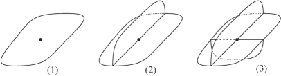
Figure 6. Local structure of an almost-special polyhedron.

Besides the set $V(P)$ of vertices already introduced above for simple polyhedra, we can define for an almost-special $P$ the singular set, given by the non-surface points and denoted by $S(P)$. We remark that $S(P)$ is a 4-valent graph with vertex set $V(P)$. Note also that if $P$ is an almost-special spine of $(M,G)$, by the transversality assumption, $G$ intersects $P$ away from $S(P)$.

An almost-special polyhedron $P$ is called special if $P\setminus S(P)$ is a union of open discs and $S(P)\setminus V(P)$ is a union of open segments. A special spine of a graph $(M,G)$ is a simple spine which, in addition, is a special polyhedron.

The following result, which refers to the case of manifolds without graphs embedded in them, has been known for a long time. We point out that we use the term triangulation for a (closed, connected, orientable) $3$-manifold $M$ in a generalized (not strictly PL [44]) sense. Namely, we mean a realization of $M$ as a simplicial pairing between the faces of a finite union of tetrahedra, i.e., we allow multiple and self-adjacencies between tetrahedra.

Proposition 3.2.

Given a $3$-manifold $M$, for each triangulation ${\mathcal{T}}$ of $M$ define $\Phi({\mathcal{T}})$ as the $2$-skeleton of the cell decomposition dual to ${\mathcal{T}}$, see Figure 7.

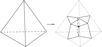
Figure 7. Duality between triangulations and special spines.

Then $\Phi$ defines a bijection between the set of (isotopy classes of) triangulations of $M$ and the set of (isotopy classes of) special spines of $M$.

3.3. (Efficient) triangulations of graphs

We now turn to graphs $(M,G)$, and we define a triangulation of $(M,G)$ to be a (generalized) triangulation ${\mathcal{T}}$ of $M$ which contains $G$ as a subset of its 1-skeleton. We will further say that ${\mathcal{T}}$ is efficient if it has precisely one vertex at each vertex of $G$, one on each knot component of $G$, and no other vertices.

The following easy result shows that under suitable conditions Proposition 3.2 has a refinement to graphs:

Proposition 3.3.

For a simple spine $P$ of a graph $(M,G)$ the following conditions are equivalent:

• $P$ is dual to a triangulation of $(M,G)$;

• $P$ is special, $G$ intersects $P$ transversely away from $S(P)$, and each component of $P\setminus S(P)$ intersects $G$ at most once.

3.4. Minimal spines

A simple spine $P$ of a graph $(M,G)$ is called minimal if it has $c(M,G)$ vertices and no subset of $P$ is also a spine of $(M,G)$. The success of the strategy based on complexity theory (as outlined at the beginning of this section) for the enumeration of hyperbolic graphs depends on the next three results. They require the concept of $(0,1,2)$-irreducibility defined in the introduction. The first one is part of Theorem 2.4, the next two easily follow from [41, Theorem 2.6].

Proposition 3.4.

If $(M,G)$ is hyperbolic with parabolic meridians then $(M,G)$ is $(0,1,2)$-irreducible.

Proposition 3.5.

The $(0,1,2)$-irreducible graphs $(M,G)$ with $c(M,G)=0$ are those described as follows and illustrated in Figure 8:

• $M$ is either $S^{3}$, or $L(3,1)$, or ${\mathbb{P}}^{3}$, and $G$ is either empty or the core of a Heegaard solid torus of $M$;

• $M$ is $S^{3}$ and $G$ is the trivially embedded $\theta$-graph.

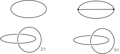
Figure 8. The $(0,1,2)$-irreducible graphs of complexity 0. Here and below a knot component carrying a fractional label should be understood as a surgery instruction [43]. In particular, it is not actually part of the graph.

Theorem 3.6.

Let $(M,G)$ be a graph with $c(M,G)>0$. Then the following are equivalent:

• $(M,G)$ is $(0,1,2)$-irreducible;

• $(M,G)$ admits a special minimal spine;

• Every minimal spine of $(M,G)$ is special and dual to it there is an efficient triangulation of $(M,G)$.

3.5. Non-minimality criteria

The following result was used for the enumeration of candidate triangulations of $(0,1,2)$-irreducible graphs, as explained in more detail in the next section:

Proposition 3.7.

Let ${\mathcal{T}}$ be a triangulation of a graph $(M,G)$, and let $P$ be the special spine dual to ${\mathcal{T}}$. Suppose that in ${\mathcal{T}}$ there is an edge not lying in $G$ and incident to $i$ distinct tetrahedra, with $i\leqslant 3$. Then $P$ is not minimal.

Proof.

We will show that we can perform a move on $P$ leading to a simple spine of $(M,G)$ with fewer vertices than $P$.

For $i=3$ we do not even need to use spines, the move exists already at the level of triangulations: it is the famous Matveev-Piergallini $3\to 2$ move [33, 42] illustrated in Figure 9. We only need to note that after the move we still have a triangulation of $(M,G)$ because the edge that disappears with the move does not lie in $G$.

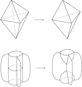
Figure 9. The $3\to 2$ move on triangulations and its dual version for spines.

For $i=1,2$ we do need to use spines. The moves we apply (a $1\to 0$ and a $2\to 0$ move) are illustrated in Figure 10. Both moves involve the removal of the component $R$ of $P\setminus S(P)$ dual to the edge of the statement, and the result of the move is still a spine of $(M,G)$ because $G$ does not meet $R$. We note that the $2\to 0$ move leads to an almost-special polyhedron, but it can create a spine with an annular non-singular component, in which case the spine is not dual to a triangulation. The $1\to 0$ move gives a spine which is not almost-special. ∎

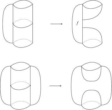
Figure 10. The $1\to 0$ and the $2\to 0$ moves on spines. Both these moves transform a special spine $P$ into a simple spine which is not necessarily special. If $P$ has at least $2$ vertices, both moves destroy at least 2 vertices of $P$: the $2\to 0$ move destroys precisely two; the $1\to 0$ move can be completed by collapsing the face $f$, which is necessarily adjacent to at least another vertex of $P$ that disappears after the collapse.

Remark 3.8.

Sometimes the non-minimality criteria of the previous proposition do not apply directly, but only after a modification of the triangulation. For instance, a triangulation $T$ with $n$ tetrahedra may be transformed into one $T^{\prime}$ with $n+1$ tetrahedra via a $2\to 3$ move: if $T^{\prime}$ contains an edge incident to $1$ or $2$ distinct tetrahedra, the dual spine $P^{\prime}$ can be transformed into a simple spine with at most $n-1$ vertices by applying one of the moves in Figure 10. Therefore the original triangulation $T$ is not minimal.

3.6. Complexity of the complement

Matveev’s complexity [32] is defined for every compact $3$-manifold, with or without boundary. The complement $X$ of an open regular neighbourhood of a graph $G$ in a closed $3$-manifold $M$ therefore has a complexity, which is related to $c(M,G)$ as follows.

Proposition 3.9.

For any graph $(M,G)$ we have

$$c\big{(}X)\leqslant c(M,G).$$

If $(M,G)$ is $(0,1,2)$-irreducible with $c(M,G)\neq 0$ and $G\neq\emptyset$, then

$$c(X)<c(M,G).$$

Proof.

If $P$ is a minimal simple spine of $(M,G)$ then the graph $G$ intersects $P$ in a finite number of points. Removing from $P$ open regular neighbourhoods of these points gives a simple polyhedron $P^{\prime}\subset P$ which is a spine of $X$ with the same vertices as $P$. Therefore $c\big{(}X)\leqslant c(M,G)$.

If $(M,G)$ is $(0,1,2)$-irreducible, $G\neq\emptyset$ and $c(M,G)\neq 0$, then Theorem 3.6 shows that a minimal simple spine $P$ of $(M,G)$ is special and $G\cap P$ consists of some $k\geqslant 1$ points belonging to the interior of $k$ distinct disc components of $P\setminus S(P)$. Removing these $k$ discs we get a simple spine of $X$ with strictly fewer vertices than $P$. ∎

Remark 3.10.

A compact $3$-manifold which admits a complete hyperbolic metric with geodesic boundary and finite volume (after removing the tori from its boundary) has complexity at least $2$, see [32, 2, 11]. This explains why the first hyperbolic knots $(M,G)$ have $c(M,G)\geqslant 3$ (see Tables 1 and 2). Analogously, the first graphs $(M,G)$ whose complement is hyperbolic with geodesic boundary must have $c(M,G)\geqslant 3$. (In fact they have complexity $5$, see Subsection 5.4.)

4. Computer programs and obstructions to hyperbolicity

In this section we describe the Haskell code we have written to enumerate triangulations, and the computer program Orb we have used to investigate hyperbolic structures. We also describe how non-hyperbolic graphs were identified (see also Section 6 below).

4.1. Enumeration of marked triangulations

Thanks to Theorem 3.6 and the other results stated in the previous section, the enumeration of $(0,1,2)$-irreducible graphs of complexity $n$ can be performed by listing all efficient triangulations with $n$ tetrahedra satisfying some minimality criteria. This was done via a separate program, written in Haskell [18], which suitably adapts the strategy already used in similar censuses (e.g. [30, 35]).

A triangulation of a graph $(M,G)$ can be encoded as a triangulation of $M$ with some marked edges. A triangulation here is just a gluing of tetrahedra, which can be described via a connected $4$-valent graph (the incidence graph of the gluing) having a label on each edge encoding how the corresponding triangular faces are identified (there are $3!=6$ possibilities).

A first count gives $c_{n}\cdot 6^{2n}=c_{n}\cdot 36^{n}$ triangulations to check, where $c_{n}$ is the number of $4$-valent graphs with $n$ vertices (and $2n$ edges), shown in Table 3. On each triangulation there are $2^{e}=2^{n+v}$ distinct markings of edges, where $e$ is the number of edges and $v$ is the number of vertices in the triangulation of $M$. Since there are at least $2$ triangles in the link of each vertex, $v\leqslant 2n$, and $e\leqslant 3n$. There are therefore up to $c_{n}\cdot 36^{n}\cdot 2^{3n}=c_{n}\cdot 288^{n}$ marked triangulations to check. This number is already too big for $n=3$, so in order to simplify the problem we used some tricks.

$n$	$1$	$2$	$3$	$4$	$5$
$c_{n}$	$1$	$2$	$4$	$10$	$28$
$c_{n}^{\prime}$	$1$	$3$	$5$	$18$	$56$

Table 3. The number $c_{n}$ of $4$-valent graphs with $n$ vertices, and $c_{n}^{\prime}$ of $4$-valent graphs with oriented vertices.

We are only interested in orientable manifolds $M$. We can therefore orient each tetrahedron and require the identifications of faces to be orientation-reversing. This reduces the number of possible labels on edges from $6$ to $3$, and the number of triangulations to $c_{n}^{\prime}\cdot 3^{2n}=c_{n}^{\prime}\cdot 9^{n}$, where $c_{n}^{\prime}$ is the number of $4$-valent graphs with “oriented” vertices: each vertex has a fixed parity of orderings of the incident edges. For a fixed $4$-valent graph $G$ with $n$ vertices, the vertices can be oriented in $2^{n}$ different ways, but up to the symmetries of $G$ the number of distinct orientations typically turns out to be very small. This explains why $c_{n}^{\prime}$ is actually much less than $2^{n}\cdot c_{n}$, as shown in the table.

We selected from the resulting list of triangulations only those yielding closed manifolds. Finally, on each triangulation we a priori had $2^{e}$ distinct markings on edges to analyze. Proposition 3.7 was used to discard many of these: in a triangulation dual to a minimal spine an edge incident to at most $3$ distinct tetrahedra is necessarily marked. It remained then to check which markings give rise to efficient triangulations.

4.2. “Orb”

Hyperbolic structures were computed using the program Orb written by Damian Heard [20, 19]. This program builds on ideas of Thurston, Weeks, Casson and others to find hyperbolic structures and associated geometric invariants for a large class of 3-dimensional manifolds and orbifolds. The program begins with a triangulation of the space with the singular locus or graph contained in the 1-skeleton and tries to find shapes of generalized hyperbolic tetrahedra (with vertices inside, on, or outside the sphere at infinity) which fit together to give a hyperbolic structure.

The generalized hyperbolic tetrahedra are described by using one parameter for each edge in the triangulation. For a general tetrahedron a lift to Minkowski space is chosen, then the parameters are Minkowski inner products of the vertex positions. For compact tetrahedra, each parameter is just the hyperbolic cosine of the edge length. For each ideal vertex the lift to Minkowski space determines a horosphere centred at the vertex; for each hyperideal vertex a geodesic plane orthogonal to the incident faces is determined. Then the edge parameters are simple functions of the hyperbolic distances between these surfaces.

Given the edge parameters, all dihedral angles of the tetrahedra are determined. Moreover the parameters give a global hyperbolic structure if and only if the sum of the dihedral angles around each edge is $2\pi$ (or the desired cone angle, in the orbifold case). This gives a system of equations that Orb solves numerically using Newton’s method, starting with suitable regular generalized tetrahedra as the initial guess.

Once a hyperbolic structure is found, Orb can compute many geometric invariants including volumes, the Kojima canonical decompositions, and symmetry groups. This uses methods based on ideas of Weeks [52], Ushijima [50] and Frigerio-Petronio [12], too complicated to be reproduced here.

After computing hyperbolic structures numerically using Orb, we checked the correctness of the results by using Jeff Weeks’ program SnapPea [51] to calculate complete hyperbolic structures on the manifolds with torus cusps obtained by doubling along all 3-punctured sphere boundary components.

Finally, we verified the results by using Oliver Goodman’s program Snap [17, 8] to find exact hyperbolic structures. This provides a proof that the hyperbolic structures are correct and allows us to compute associated arithmetic invariants (including invariant trace fields), as already mentioned in Subsection 2.6 above.

4.3. Non-hyperbolic knots and links

Many knots and links in the census turned out to be torus links in lens spaces, see Subsection 6.1 below. From $c=3$, we then decided to rule out the non-hyperbolic knots and links from our census (except for those in $S^{3}$ at $c=3$); this helped a lot in simplifying the classification. Many non-hyperbolic knots and links were easily identified by the following criterion:

Remark 4.1.

If the complexity of the complement is at most $1$ then the link is not hyperbolic by Remark 3.10. This holds for instance if there are $n$ tetrahedra and the marked edge of the triangulation is incident to at least $n-1$ of them (see the proof of Proposition 3.9).

The remaining knots and links were shown to be non-hyperbolic by examining their fundamental groups with the help of the following observations.

Lemma 4.2.

Let $M$ be an orientable finite volume hyperbolic $3$-manifold, and let $a,b,c\in\pi_{1}(M)$. Then

1. if $[a^{p},b^{q}]=1$ for some integers $p,q\neq 0$ then $[a,b]=1$,

2. if $[a,b]=1$ and $b=cac^{-1}$ then $a=b$.

Proof.

The results are clear if $a,b$ or $c$ is the identity, so we may assume that $a,b$ and $c$ correspond to loxodromic or parabolic isometries of ${\mathbb{H}}^{3}$.

In part (i), the elements $a^{p},b^{q}$ must have the same axis or fixed point at $\infty$. Since $p,q\neq 0$ the same is true for $a$ and $b$, so $a$ and $b$ commute.

In part (ii), $a$ and $b$ have the same fixed point set $F$ on the sphere at infinity, and $c$ takes $F$ to itself. Since $c$ is not elliptic, it must fix each point of $F$. Thus $c$ has the same axis or fixed point at $\infty$ as $a$ and $b$, so it commutes with them.∎

Lemma 4.3.

Let $M$ be an orientable finite volume hyperbolic $3$-manifold. Then $\pi_{1}(M)$ cannot have a presentation of the form

1. $\langle a,b\mid a^{n}(a^{p}b^{q})^{k}=1\rangle$ where $k,n,p,q$ are integers with $k,n,q\neq 0$, or

2. $\langle a,b\mid a^{2}b^{-1}a^{-1}b^{2}a^{-1}b^{-1}=1\rangle$.

Proof.

(i) If $a^{n}(a^{p}b^{q})^{k}=1$, then $[a^{n},a^{p}b^{q}]=1$ by part (i) of Lemma 4.2. Hence $[a^{n},b^{q}]=1$ and $[a,b]=1$, again by part (i) of Lemma 4.2. So the group would be abelian, which is impossible.

(ii) The group has a presentation

$$\langle a,b,x,y\mid x=ab^{-1},y=a^{-1}b,[x,y]=1\rangle.$$

We can rewrite this as

$$\langle a,x,y\mid x=ay^{-1}a^{-1},[x,y]=1\rangle.$$

Hence $x=y^{-1}$ by part (ii) of Lemma 4.2 and $[a,x]=1$. So the group would be abelian, which is again impossible. ∎

Among the knots and links up to complexity 4 for which Orb did not find a hyperbolic structure, all but one of the complements had a fundamental group with presentation of the form $\langle a,b\mid[a^{n},b^{m}]=1\rangle$, or $\langle a,b\mid a^{n}(a^{p}b^{q})^{k}=1\rangle$. These all correspond to non-hyperbolic links by the Lemmas above. The one remaining knot had a presentation as in part (ii) of Lemma 4.3, so is also non-hyperbolic.

4.4. Non-hyperbolic graphs

For graphs with at least one vertex, we first eliminated all triangulations whose dual spines had non-minimal complexity hence were either reducible or occurred earlier in our list. This left a handful of examples for which Orb failed to find a hyperbolic structure. These were first examined using Jeff Weeks’ program SnapPea, by constructing triangulations of the manifolds with torus cusps obtained by doubling along the 3-punctured sphere boundary components. We used SnapPea’s “splitting” function to look for incompressible Klein bottles and tori in the doubles. This suggested that incompressible Klein bottles were present in the original graph complements. We then verified this and showed that these examples were indeed non-hyperbolic by theoretical means, as explained below in Section 6.

5. Hyperbolic census details

In this section we will expand on the information given in Table 1, providing details of all the 123 hyperbolic graphs up to complexity 5. Pictures of the hyperbolic graphs up to complexity 4 will be shown in Section 7.

5.1. Name conventions

For future reference, we have chosen a name for each of the graphs we have found. The name has the form

$$ng\_\,c\_\,i$$

where $n$ is the number of vertices of the graph, $g$ is a string describing the abstract graph type, $c$ is the complexity, and $i$ is an index (starting from $1$ for any given $ng\_\,c$). We have found in our hyperbolic census only 6 graph types, described above in Figure 2, so a string of one letter only (or the empty string, for knots) was sufficient to identify them. For graphs with 2 vertices, the letters $t$ and $h$ were suggested by the common names “$\theta$-graph” and “handcuffs”. The choice of letters was arbitrary for graphs with $4$ vertices.

5.2. Organization of tables

We will give separate tables for $\theta$-graphs, handcuffs, $4$-vertex graphs, and knots. Within each table, graphs are always arranged in increasing order of their hyperbolic volumes. For graphs having vertices, the columns of the tables respectively contain:

1. The name of the graph $(M,G)$.

2. The volume of the hyperbolic structure with parabolic meridians on $M\setminus G$.

3. A description of the cells of the Kojima canonical decomposition for this structure. When all these cells are tetrahedra we simply indicate their number, otherwise we add an asterisk in the table and provide additional information separately.

4. The symmetry group of $(M,G)$, with $D_{n}$ denoting the dihedral group with $2n$ elements.

5. Whether $(M,G)$ is chiral (c) or amphichiral (a).

6. The name of the underlying space $M$. This is almost always a lens space; otherwise it is a Seifert fibred space which we describe in the usual way (as in [34, p. 406]).

7. The degree, signature and discriminant of the invariant trace field. Details of minimal polynomials for the fields are available on the web at www.ms.unimelb.edu.au/~snap/knotted_graphs.html.

8. Whether all traces of group elements are algebraic integers.

9. Whether the group is arithmetic (after doubling to obtain a finite covolume group).

name	volume	(K)	sym	a/c	space	deg	sig	disc	int	ar
$2t\_\,2\_\,1$	5.333489567	3	$D_{2}$	c	$S^{3}$	2	0, 1	$-$7	Y	Y
$2t\_\,2\_\,2$	5.333489567	3	$D_{6}$	c	$L$(3,1)	2	0, 1	$-$7	Y	Y
$2t\_\,3\_\,1$	6.354586557	4	$D_{2}$	c	${\mathbb{P}}^{3}$	3	1, 1	$-$44	Y	N
$2t\_\,3\_\,2$	6.354586557	4	$D_{2}$	c	$L$(4,1)	3	1, 1	$-$44	Y	N
$2t\_\,3\_\,3$	6.551743288	7	$D_{2}$	c	$S^{3}$	3	1, 1	$-$107	Y	N
$2t\_\,3\_\,4$	6.551743288	7	$D_{2}$	c	$L$(5,2)	3	1, 1	$-$107	Y	N
$2t\_\,4\_\,1$	6.755194816	5	$D_{2}$	c	$L$(3,1)	4	0, 2	2917	Y	N
$2t\_\,4\_\,2$	6.755194816	5	$D_{2}$	c	$L$(5,1)	4	0, 2	2917	Y	N
$2t\_\,4\_\,3$	6.927377112	11	$D_{2}$	c	$S^{3}$	4	0, 2	1929	Y	N
$2t\_\,4\_\,4$	6.927377112	11	$D_{2}$	c	$L$(7,3)	4	0, 2	1929	Y	N
$2t\_\,5\_\,1$	6.952347978	6	$D_{2}$	c	$L$(4,1)	5	1, 2	7684	Y	N
$2t\_\,5\_\,2$	6.952347978	6	$D_{2}$	c	$L$(6,1)	5	1, 2	7684	Y	N
$2t\_\,4\_\,5$	6.987763199	7	$D_{2}$	c	$L$(3,1)	5	1, 2	77041	Y	N
$2t\_\,4\_\,6$	6.987763199	7	$D_{2}$	c	$L$(7,2)	5	1, 2	77041	Y	N
$2t\_\,4\_\,7$	7.035521457	8	$D_{2}$	c	${\mathbb{P}}^{3}$	5	1, 2	5584	Y	N
$2t\_\,4\_\,8$	7.035521457	8	$D_{2}$	c	$L$(8,3)	5	1, 2	5584	Y	N
$2t\_\,5\_\,3$	7.084790037	15	$D_{2}$	c	$S^{3}$	5	1, 2	49697	Y	N
$2t\_\,5\_\,4$	7.084790037	15	$D_{2}$	c	$L$(9,2)	5	1, 2	49697	Y	N
$2t\_\,5\_\,5$	7.142157274	9	$D_{2}$	c	$L$(5,2)	7	1, 3	$-$123782683	Y	N
$2t\_\,5\_\,6$	7.142157274	9	$D_{2}$	c	$L$(9,2)	7	1, 3	$-$123782683	Y	N
$2t\_\,5\_\,7$	7.157517365	8	$D_{2}$	c	$L$(4,1)	7	1, 3	$-$2369276	Y	N
$2t\_\,5\_\,8$	7.157517365	8	$D_{2}$	c	$L$(10,3)	7	1, 3	$-$2369276	Y	N
$2t\_\,5\_\,9$	7.175425922	9	$D_{2}$	c	$L$(3,1)	7	1, 3	$-$88148831	Y	N
$2t\_\,5\_\,10$	7.175425922	9	$D_{2}$	c	$L$(11,3)	7	1, 3	$-$88148831	Y	N
$2t\_\,5\_\,11$	7.192635929	11	$D_{2}$	c	$L$(5,2)	8	0, 4	5442461517	Y	N
$2t\_\,5\_\,12$	7.192635929	11	$D_{2}$	c	$L$(11,3)	8	0, 4	5442461517	Y	N
$2t\_\,5\_\,13$	7.193764490	12	$D_{2}$	c	${\mathbb{P}}^{3}$	7	1, 3	$-$1523968	Y	N
$2t\_\,5\_\,14$	7.193764490	12	$D_{2}$	c	$L$(12,5)	7	1, 3	$-$1523968	Y	N
$2t\_\,5\_\,15$	7.216515907	11	$D_{2}$	c	$L$(3,1)	8	0, 4	3679703653	Y	N
$2t\_\,5\_\,16$	7.216515907	11	$D_{2}$	c	$L$(13,5)	8	0, 4	3679703653	Y	N
$2t\_\,4\_\,9$	7.327724753	4	$D_{2}$	a	$S^{2}\times S^{1}$	2	0, 1	$-$4	Y	Y
$2t\_\,4\_\,10$	7.517689896	6	$D_{2}$	c	$L$(3,1)	3	1, 1	-104	Y	N
$2t\_\,4\_\,11$	7.706911803	5	$D_{2}$	c	$S^{3}$	3	1, 1	$-$59	Y	N
$2t\_\,4\_\,12$	7.706911803	5	$D_{2}$	c	$L$(5,1)	3	1, 1	$-$59	Y	N
$2t\_\,4\_\,13$	7.867901276	7	${\mathbb{Z}}_{2}$	c	$L$(7,2)	5	3, 1	-112919	Y	N
$2t\_\,4\_\,14$	7.940579248	9	$D_{2}$	c	$L$(8,3)	3	1, 1	-76	Y	N
$2t\_\,4\_\,15$	7.940579248	9	$D_{6}$	c	$S^{3}/Q_{8}$	3	1, 1	-76	Y	N
$2t\_\,4\_\,16$	8.000234350	4	$D_{2}$	c	${\mathbb{P}}^{3}$	2	0, 1	$-$7	Y	Y
$2t\_\,5\_\,17$	8.087973789	5	${\mathbb{Z}}_{2}$	c	$S^{3}$	4	2, 1	$-$6724	Y	N
$2t\_\,5\_\,18$	8.195703083	7	${\mathbb{Z}}_{2}$	c	$L$(5,2)	5	1, 2	65516	Y	N
$2t\_\,5\_\,19$	8.233665208	6	${\mathbb{Z}}_{2}$	c	$L$(6,1)	6	2, 2	1738384	Y	N
$2t\_\,5\_\,20$	8.338374585	8	${\mathbb{Z}}_{2}$	c	$L$(9,2)	6	2, 2	2463644	Y	N
$2t\_\,5\_\,21$	8.355502146	8	${\mathbb{Z}}_{2}$	c	$S^{3}$	4	0, 2	3173	Y	N
$2t\_\,4\_\,17$	8.355502146	6	${\mathbb{Z}}_{2}$	c	$S^{3}$	4	0, 2	3173	Y	N
$2t\_\,5\_\,22$	8.372209945	8	${\mathbb{Z}}_{2}$	c	$L$(10,3)	7	3, 2	87357184	Y	N
$2t\_\,5\_\,23$	8.388819035	10	${\mathbb{Z}}_{2}$	c	$L$(4,1)	5	1, 2	26084	Y	N

Table 4. Information on hyperbolic $\theta$-graphs up to complexity 5, table 1 of 2. Here $Q_{8}$ denotes the quaternionic group of order $8$ and $S^{3}/Q_{8}$ is the Seifert fibred space $\big{(}S^{2};(2,-1),(2,1),(2,1)\big{)}$.

name	volume	(K)	sym	a/c	space	deg	sig	disc	int	ar
$2t\_\,5\_\,24$	8.403864479	10	${\mathbb{Z}}_{2}$	c	$L$(11,3)	7	3, 2	186794473	Y	N
$2t\_\,5\_\,25$	8.487060022	8	${\mathbb{Z}}_{2}$	c	$L$(9,2)	8	4, 2	17112324248	Y	N
$2t\_\,5\_\,26$	8.527312899	10	${\mathbb{Z}}_{2}$	c	$L$(11,3)	9	5, 2	5328053407637	Y	N
$2t\_\,5\_\,27$	8.546347793	11	${\mathbb{Z}}_{2}$	c	$L$(12,5)	8	4, 2	2498992192	Y	N
$2t\_\,5\_\,28$	8.565387019	12	${\mathbb{Z}}_{2}$	c	$L$(13,5)	9	5, 2	1944699708173	Y	N
$2t\_\,5\_\,29$	8.612415201	1*	$D_{2}$	c	$L$(4,1)	4	2, 1	$-$400	Y	N
$2t\_\,5\_\,30$	8.778658803	9	$D_{2}$	c	${\mathbb{P}}^{3}$	5	1, 2	15856	Y	N
$2t\_\,5\_\,31$	8.778658803	9	$D_{2}$	c	$S^{3}/Q_{12}$	5	1, 2	15856	Y	N
$2t\_\,5\_\,32$	8.793345604	7	$D_{2}$	c	$S^{3}$	4	0, 2	257	Y	N
$2t\_\,5\_\,33$	8.806310033	8	$D_{2}$	c	$L$(8,3)	4	2, 1	$-$1968	Y	N
$2t\_\,5\_\,34$	8.908747390	11	$D_{2}$	c	$L$(3,1)	5	1, 2	31048	Y	N
$2t\_\,4\_\,18$	8.929317823	6	$D_{2}$	c	$S^{3}$	3	1, 1	$-$116	Y	N
$2t\_\,5\_\,35$	8.967360849	7	$D_{2}$	c	$S^{3}$	4	0, 2	697	Y	N
$2t\_\,5\_\,36$	8.967360849	7	$D_{2}$	c	$L$(7,2)	4	0, 2	697	Y	N
$2t\_\,5\_\,37$	9.045557688	5	${\mathbb{Z}}_{2}$	c	$L$(3,1)	5	1, 2	73532	Y	N
$2t\_\,5\_\,38$	9.272866192	7	${\mathbb{Z}}_{2}$	c	$S^{3}$	6	0, 3	$-$4319731	Y	N
$2t\_\,5\_\,39$	9.353881135	7	${\mathbb{Z}}_{2}$	c	$L$(3,1)	6	0, 3	$-$2944468	Y	N
$2t\_\,5\_\,40$	9.437583617	9	${\mathbb{Z}}_{2}$	c	${\mathbb{P}}^{3}$	4	0, 2	2312	Y	N
$2t\_\,5\_\,41$	9.491889687	5	$D_{2}$	c	$S^{3}$	4	0, 2	257	Y	N
$2t\_\,5\_\,42$	9.491889687	5	$D_{2}$	c	$L$(3,1)	4	0, 2	257	Y	N
$2t\_\,5\_\,43$	9.503403931	9	${\mathbb{Z}}_{2}$	c	${\mathbb{P}}^{3}$	4	0, 2	788	N	N
$2t\_\,5\_\,44$	10.149416064	1*	$D_{2}$	c	$S^{2}\times S^{1}$	2	0, 1	$-$3	Y	Y
$2t\_\,5\_\,45$	10.396867321	6*	$D_{3}$	c	$S^{3}$	3	1, 1	$-$139	Y	N
$2t\_\,5\_\,46$	10.666979134	6	${\mathbb{Z}}_{2}$	a	$S^{3}$	2	0, 1	-7	Y	Y
$2t\_\,5\_\,47$	10.666979134	6	${\mathbb{Z}}_{2}$	c	$S^{3}$	2	0, 1	$-$7	N	N
$2t\_\,5\_\,48$	10.666979134	5	${\mathbb{Z}}_{2}$	c	$L$(3,1)	2	0, 1	-7	Y	Y
$2t\_\,5\_\,49$	10.666979134	5	${\mathbb{Z}}_{2}$	c	$L$(3,1)	2	0, 1	-7	Y	Y

Table 5. Information on hyperbolic $\theta$-graphs up to complexity 5, table 2 of 2. Here $Q_{12}$ denotes the generalized quaternionic group of order 12 and $S^{3}/Q_{12}$ is the Seifert fibred space $\big{(}S^{2};(2,-1),(2,1),(3,1)\big{)}$. The Kojima canonical decompositions of $2t\_\,5\_\,29$ and $2t\_\,5\_\,44$ consist of a cube; the decomposition of $2t\_\,5\_\,45$ is the union of five tetrahedra and an octahedron.

name	volume	(K)	sym	a/c	space	deg	sig	disc	int	ar
$2h$_ 1_ 1	3.663862377	1	$D_{4}$	a	$S^{3}$	2	0, 1	-4	Y	Y
$2h$_ 2_ 1	5.074708032	2	$D_{4}$	a	${\mathbb{P}}^{3}$	2	0, 1	$-$3	Y	Y
$2h$_ 3_ 1	5.875918083	3	$D_{2}$	c	$L($3,1)	4	0, 2	656	Y	N
$2h$_ 3_ 2	6.138138789	5	$D_{2}$	c	$S^{3}$	4	0, 2	320	Y	N
$2h$_ 4_ 1	6.354586557	4	$D_{2}$	c	$L($4,1)	3	1, 1	-44	Y	N
$2h$_ 4_ 2	6.559335883	5	$D_{2}$	c	$L($3,1)	6	0, 3	$-$382208	Y	N
$2h$_ 5_ 1	6.647203159	5	$D_{2}$	c	$L($5,1)	6	0, 3	$-$242752	Y	N
$2h$_ 4_ 3	6.784755787	9	$D_{2}$	c	$S^{3}$	6	0, 3	$-$108544	Y	N
$2h$_ 4_ 4	6.831770496	6	$D_{2}$	c	${\mathbb{P}}^{3}$	4	0, 2	892	Y	N
$2h$_ 5_ 2	6.854770090	7	$D_{2}$	c	$L($5,2)	8	0, 4	502248448	Y	N
$2h$_ 5_ 3	6.952347978	6	$D_{2}$	c	$L($4,1)	5	1, 2	7684	Y	N
$2h$_ 5_ 4	6.969842840	5	${\mathbb{Z}}_{4}$	a	$L($5,2)	6	0, 3	$-$179776	Y	N
$2h$_ 5_ 5	7.008125009	9	$D_{2}$	c	$L($5,2)	10	0, 5	$-$1192884600832	Y	N
$2h$_ 5_ 6	7.020614792	13	$D_{2}$	c	$S^{3}$	8	0, 4	89276416	Y	N
$2h$_ 5_ 7	7.056979121	7	$D_{2}$	c	$L($3,1)	10	0, 5	$-$586177642496	Y	N
$2h$_ 5_ 8	7.136868364	10	$D_{2}$	c	${\mathbb{P}}^{3}$	6	0, 3	$-$682736	Y	N
$2h$_ 5_ 9	7.146107337	9	$D_{2}$	c	$L($3,1)	12	0, 6	8746362208256	Y	N
$2h$_ 3_ 3	7.327724753	4	$D_{2}$	a	$S^{3}$	2	0, 1	$-$4	Y	Y
$2h$_ 4_ 5	7.327724753	4	$D_{2}$	a	$S^{2}\times S^{1}$	2	0, 1	$-$4	Y	Y
$2h$_ 5_ 10	7.731874058	5	${\mathbb{Z}}_{2}$	c	$L($4,1)	6	0, 3	$-$96512	Y	N
$2h$_ 5_ 11	8.140719221	6	${\mathbb{Z}}_{2}$	c	$S^{3}$	6	0, 3	$-$382208	Y	N
$2h$_ 5_ 12	8.140719221	5	${\mathbb{Z}}_{2}$	c	$S^{3}$	6	0, 3	$-$382208	Y	N
$2h$_ 4_ 6	8.738570409	4	${\mathbb{Z}}_{2}$	a	${\mathbb{P}}^{3}$	4	0, 2	144	Y	N
$2h$_ 5_ 13	8.997351944	3*	${\mathbb{Z}}_{2}$	c	$S^{3}$	4	0, 2	784	Y	N
$2h$_ 4_ 7	8.997351944	4	$\{{\rm id}\}$	c	$S^{3}$	4	0, 2	784	Y	N
$2h$_ 4_ 8	8.997351944	4	${\mathbb{Z}}_{2}$	c	$L($3,1)	4	0, 2	784	Y	N
$2h$_ 5_ 14	9.539780459	5	$\{{\rm id}\}$	c	$L($3,1)	4	0, 2	656	Y	N
$2h$_ 5_ 15	9.539780459	5	$D_{2}$	c	$S^{3}$	4	0, 2	656	Y	N
$2h$_ 5_ 16	9.592627932	6	$D_{2}$	c	${\mathbb{P}}^{3}$	4	0, 2	1436	Y	N
$2h$_ 5_ 17	9.802001166	5	$\{{\rm id}\}$	c	$S^{3}$	4	0, 2	320	N	N
$2h$_ 5_ 18	9.876829057	5	${\mathbb{Z}}_{2}$	c	$S^{3}$	6	0, 3	$-$239168	Y	N
$2h$_ 5_ 19	10.018448934	5	$\{{\rm id}\}$	c	${\mathbb{P}}^{3}$	6	0, 3	$-$30976	N	N
$2h$_ 5_ 20	10.018448934	5	$\{{\rm id}\}$	c	$L($4,1)	6	0, 3	$-$30976	Y	N
$2h$_ 5_ 21	10.018448934	5	${\mathbb{Z}}_{2}$	c	$L($4,1)	6	0, 3	$-$30976	Y	N
$2h$_ 5_ 22	10.069070958	7	${\mathbb{Z}}_{2}$	c	${\mathbb{P}}^{3}$	4	0, 2	1384	Y	N
$2h$_ 5_ 23	10.149416064	4*	${\mathbb{Z}}_{2}$	c	$S^{2}\times S^{1}$	2	0, 1	$-$3	Y	Y
$2h$_ 5_ 24	10.215605665	5	$\{{\rm id}\}$	c	$S^{3}$	6	0, 3	$-$732736	N	N
$2h$_ 5_ 25	10.215605665	5	$\{{\rm id}\}$	c	$L($5,2)	6	0, 3	$-$732736	Y	N
$2h$_ 5_ 26	10.215605665	5	${\mathbb{Z}}_{2}$	c	$L($5,2)	6	0, 3	$-$732736	Y	N
$2h$_ 5_ 27	10.408197599	5	$\{{\rm id}\}$	c	${\mathbb{P}}^{3}$	4	0, 2	441	N	N

Table 6. Information on hyperbolic handcuff graphs up to complexity 5. The Kojima canonical decomposition of $2h$_ 5_ 13 is the union of a tetrahedron and two pyramids with square base; the decomposition for $2h$_ 5_ 23 is the union of two tetrahedra and two pyramids with square base.

name	volume	(K)	sym	a/c	space	deg	sig	disc	int	ar
$4a$_ 2_ 1	7.327724753	2	${\mathbb{Z}}_{2}\times O$	a	$S^{3}$	2	0, 1	$-$4	Y	Y
$4a$_ 5_ 1	11.751836165	6	$D_{4}$	c	$S^{3}$	4	0, 2	656	Y	N
$4a$_ 5_ 2	12.661214320	5	${\mathbb{Z}}_{2}$	c	$S^{3}$	4	0, 2	784	Y	N
$4b$_ 4_ 1	10.149416064	4	${\mathbb{Z}}_{2}\times D_{4}$	a	$S^{3}$	2	0, 1	-3	Y	Y
$4c$_ 4_ 1	10.991587130	4	$D_{2}$	a	$S^{3}$	2	0, 1	-4	Y	Y

Table 7. Information on hyperbolic 4-vertex graphs up to complexity 5. Here $O$ denotes the group of orientation-preserving symmetries of the regular octahedron, isomorphic to the full group of symmetries of the regular tetrahedron.

5.3. Table of knots

As already mentioned, we have classified hyperbolic knots only up to complexity 4, finding 5 of them. The table containing their description differs from the previous ones only in that the third column gives the number of cells in the Epstein-Penner [9] canonical decomposition (the Kojima decomposition is not defined). We also provide an additional table showing the name of each knot complement in the SnapPea census [2], and either the name of the knot in [43] (for the knots in $S^{3}$) or the surgery coefficients on one of the components of the Whitehead link ($5_{1}^{2}$ in [43]) yielding the knot.

As shown in the introduction and in Section 6 below, there are many $(0,1,2)$-irreducible knots in complexity up to $3$, and most of them are not hyperbolic: this phenomenon can be understood using spines, see Proposition 3.9.

name	volume	(EP)	sym	a/c	space	deg	sig	disc	int	ar
0_ 3_ 1	2.029883213	2	$D_{4}$	a	$S^{3}$	2	0,1	$-$3	Y	Y
0_ 4_ 1	2.029883213	2	$D_{2}$	c	$L(5,1)$	2	0,1	$-$3	Y	Y
0_ 4_ 2	2.568970601	4	$D_{2}$	c	$L(3,1)$	3	1,1	$-$59	Y	N
0_ 4_ 3	2.666744783	3	$D_{2}$	c	${\mathbb{P}}^{3}$	2	0,1	$-$7	Y	Y
0_ 4_ 4	2.828122088	4	$D_{2}$	c	$S^{3}$	3	1,1	$-$59	Y	N

Table 8. Information on hyperbolic knots up to complexity 4.

name	in [2]	in [43]
0_ 3_ 1	$m$004	$4_{1}$
0_ 4_ 1	$m$003	$5_{1}^{2}(-5,1)$
0_ 4_ 2	$m$007	$5_{1}^{2}(-3,2)$
0_ 4_ 3	$m$009	$5_{1}^{2}(2,1)$
0_ 4_ 4	$m$015	$5_{2}$

Table 9. Other names for hyperbolic knots up to complexity 4.

5.4. Compact totally geodesic boundary

The 3 graphs referred to in Proposition 1.1 are $2t\_\,5\_\,45$, $2t\_\,5\_\,46$ and $2t\_\,5\_\,47$ in Table 5; these are shown in Figure 3. (In particular, Thurston’s knotted $Y$ [46, pp. 133-137] is $2t\_\,5\_\,45$.) Their hyperbolic structures were constructed using Orb. They all have the lowest possible volume ($\approx 6.45199027$) for hyperbolic $3$-manifolds with genus 2 boundary (see [26]), but they can be distinguished by their Kojima decompositions or symmetry groups. All the other graphs were shown not to have such a structure by studying spines for their complements constructed as in the proof of Proposition 3.9. In all but two cases, this produced a spine for the complement of complexity having less than $2$ vertices, hence the complement has no hyperbolic structure with geodesic boundary by Remark 3.10. For the two remaining cases, we found a spine having 2 vertices but not dual to a triangulation. It again follows that these manifolds are not hyperbolic with geodesic boundary, because a minimal simple spine of a hyperbolic manifold is always dual to a triangulation [34].

6. Irreducible non-hyperbolic graphs

This section is devoted to the description of the $(0,1,2)$-irreducible but non-hyperbolic graphs we have found in our census, including the proof that indeed they have these properties.

6.1. Knots and links

As already stated in the introduction, we have shown that if a graph $(M,G)$ with $c(M,G)\leqslant 4$ is $(0,1,2)$-irreducible but non-hyperbolic then $G$ has no vertices. More precisely, $G$ is either empty, or a knot, or a two-component link. Since this paper is chiefly devoted to the understanding of graphs with vertices, we will only very briefly describe our discoveries for the case without vertices. In particular, we will not refer to the case of empty $G$ (i.e., to the case of manifolds), addressing the reader to [34], and we will describe the following non-hyperbolic knots and links:

• up to complexity $2$, in general manifolds;

• in complexity $3$, in $S^{3}$.

To proceed we will introduce some general machinery.

6.2. Torus knots in lens spaces

Consider the solid torus ${\mathbb{T}}$ and the basis of $H_{1}(\partial{\mathbb{T}})$ given by a longitude $\lambda$ and a meridian $\mu$. These elements are characterized up to symmetries of ${\mathbb{T}}$ by the property that the restriction to $\langle\lambda\rangle$ of the map $i_{*}:H_{1}(\partial{\mathbb{T}})\to H_{1}({\mathbb{T}})$ is surjective, while $\langle\mu\rangle$ is the kernel of this map.

For coprime $\ell,m\in{\mathbb{Z}}$ we will denote by $K(\ell,m)$ a simple closed curve on $\partial{\mathbb{T}}$ (unique up to isotopy) representing $\ell\cdot\lambda+m\cdot\mu$ in $H_{1}(\partial{\mathbb{T}})$. For $n\geqslant 2$ we will also denote by $K(n\cdot\ell,n\cdot m)$ the union of $n$ parallel copies of $K(\ell,m)$.

We will assume from now on that the lens space $L(p,q)$ is obtained from ${\mathbb{T}}$ by Dehn filling along $K(p,q)$. Therefore any $K(\ell,m)$ can be viewed as a torus knot on the Heegaard torus $\partial{\mathbb{T}}$ in $L(p,q)$. An easy application of the Seifert-Van Kampen theorem implies the following:

Proposition 6.1.

For $\ell,m$ coprime integers, $\pi_{1}\big{(}L(p,q)\setminus K(\ell,m)\big{)}\cong\langle x,y|\ x^{a}=y^{b}\rangle$ with $a=|\ell|$ and $b=|pm-q\ell|$.

Remark 6.2.

The curves $K(\ell,m)$ and $K(m,\ell)$ coincide as knots in $L(1,0)=S^{3}$. For instance $K(2,3)$ and $K(3,2)$ are equivalent trefoil knots in $L(1,0)=S^{3}$. This is of course consistent with the computation of the fundamental group.

Proposition 6.3.

If $(\ell,m)=(p,q)=1$ then $\big{(}L(p,q),K(\ell,m)\big{)}$ is a $(0,1,2)$-irreducible pair except in the following cases:

• $\ell=0$ or $pm-q\ell=0$, and $q\neq 0$ (i.e., $L(p,q)\neq S^{3}$);

• $|\ell|\leqslant 2$ and $p=0$ (i.e., $L(p,q)=S^{2}\times S^{1}$).

Proof.

If $\ell=0$ or $pm-q\ell=0$ then $K:=K(\ell,m)$ bounds a meridian disc of either ${\mathbb{T}}$ or the complementary solid torus attached to $\partial{\mathbb{T}}$. Therefore $K$ is the unknot, and the pair is not $0$-irreducible when $L(p,q)\neq S^{3}$. If $L(p,q)=S^{2}\times S^{1}$, the knot $K$ intersects the sphere $S^{2}\times\{pt\}$ in $|\ell|$ points. Therefore if $|\ell|\leqslant 2$ the pair is not $|\ell|$-irreducible.

Conversely, let us assume that there exists an essential sphere $S$ in $L(p,q)$ meeting $K:=K(\ell,m)$ transversely in $t\leqslant 2$ points. Suppose first that $t=0$. If $|\ell|$ and $|pm-q\ell|$ are non-zero, the complement of $K$ in $L(p,q)$ has a Seifert fibration over the disc with two singular fibers of orders $|\ell|$ and $|pm-q\ell|$: such a manifold is irreducible, so $S$ cannot be essential, a contradiction. So either $\ell=0$ or $pm-q\ell=0$, which implies that $K$ is the unknot in one of the solid tori and $S$ is the boundary of a ball containing $K$. Since $S$ is essential it follows that $M\neq S^{3}$, namely $q\neq 0$. (This argument shows in particular that when $L(p,q)=S^{2}\times S^{1}$ (i.e., $p=0$), the pair $(L(p,q),K)$ is 0-reducible only for $\ell=0$.)

Suppose now $t\neq 0$ and assume, after an isotopy, that $S$ is transverse to the Heegaard torus $\partial{\mathbb{T}}$. Considering this transverse intersection on $S$ we see that there must be at least two innermost discs. Moreover any innermost disc belongs to one of the following types:

• Its boundary is inessential on $\partial{\mathbb{T}}$ and disjoint from $K$;

• Its boundary is inessential on $\partial{\mathbb{T}}$ and meets $K$ transversely in two points;

• It is a meridian disc of either ${\mathbb{T}}$ or of the complementary solid torus.

Discs of type (I) can be removed by an isotopy. If there is a disc of type (II) then doing surgery close to it we can replace $S$ by an essential sphere disjoint from $K$, so we are led back to the case $t=0$. Therefore we can assume all the discs are of type (III). If $\ell=0$ or $pm-q\ell=0$, we can again reduce to the case $t=0$. So we can assume that all the innermost discs meet $K$, which easily implies that there are only two of them, either sharing their boundary or separated by an annulus. In the first case we see that $M=S^{2}\times S^{1}$ (i.e., $p=0$) and $1\leqslant|\ell|\leqslant 2$. In the second case we deduce that $S$ is actually inessential, which is absurd. This concludes the proof. ∎

6.3. Layered triangulations

A layered triangulation (see  [22]) of a lens space $L(p,q)$ is constructed as follows. We start with a solid torus triangulated using one tetrahedron as in Figure 11. The boundary torus is triangulated by 2 triangles, 3 edges and 1 vertex. A change of the triangulation on the boundary by a diagonal exchange move (“flip”) can be realized by adding one tetrahedron. After a series of these moves, the resulting triangulation can be closed up by adding another 1-tetrahedron triangulation of a solid torus to produce a lens space.

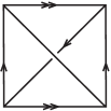
Figure 11. A 1-tetrahedron triangulation of the solid torus. The back two triangles are glued together to form a Möbius strip. The front two triangles form the boundary torus.

Such a layered triangulation of $L(p,q)$ with one vertex and one marked edge always gives rise to some torus knot $K(\ell,m)\subset L(p,q)$. Using the Farey tessellation of hyperbolic plane ${\mathbb{H}}^{2}$ we will now show the converse, namely for every torus knot $\big{(}L(p,q),K(\ell,m)\big{)}$ we will construct a layered triangulation.

Recall that the Farey tessellation of ${\mathbb{H}}^{2}$ is constructed in the half-plane model by joining with a geodesic every pair $(p/q,r/s)$ of rational ideal points in $\mathbb{Q}\cup\{\infty\}\subset\partial{\mathbb{H}}^{2}$ where $p,q,r,s$ are integers with $ps-qr=\pm 1$. After fixing some basis for $H_{1}(T)$, every slope (i.e., unoriented essential simple closed curve) on a torus $T$ is represented by a rational number $p/q\in\partial{\mathbb{H}}^{2}$, and two such numbers are connected by an edge of the tessellation when they have geometric intersection number $1$.

Every triangle of the tessellation represents three slopes with pairwise intersection $1$, and hence a $1$-vertex triangulation of $T$. Dually, they represent a $\theta$-graph in $T$ as in Figure 12-(1-top). Moreover, every edge of the tessellation represents a flip relating the $\theta$-graphs of $T$ corresponding to the adjacent triangles as in Figure 12-(2,3).

A layered triangulation of a lens space $L(p,q)$ is easily encoded via a path of triangles of the tessellation connecting the rational numbers $0/1$ and $p/q$, i.e., a sequence $f_{1},\ldots,f_{k}$ of $k\geqslant 4$ triangles such that $f_{i-1}$ and $f_{i}$ share an edge for $i=2,\ldots,k$, the vertex of $f_{1}$ disjoint from $f_{2}$ is $0/1$, and the vertex of $f_{k}$ disjoint from $f_{k-1}$ is $p/q$. The path need not to be injective, i.e., there may be repetitions. Such a path is similar to the one defined in [22, 31] for layered solid tori. It determines a layered triangulation of $L(p,q)$ with $k-3$ tetrahedra, $k-2$ edges and $1$ vertex, as described in Fig 12.

The $k-2$ edges of the layered triangulation become torus knots, and they correspond to all the slopes $\ell/m$ contained in some $f_{i}$ except $0/1$ and $p/q$. (There are $k$ different such slopes, but the two in $f_{1}$ different from $0/1$ give isotopic links in $L(p,q)$, and in fact the same edge in the layered triangulation, and similarly for the two slopes in $f_{k}$ different from $p/q$, whence the number $k-2$). See Figure 13 for some examples.

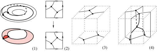
Figure 12. A path of triangles $f_{1},\ldots,f_{k}$ in the Farey tessellation determines a layered triangulation of a lens space, as follows. We describe the dual special spine. The vertices of $f_{2}$ are $1$, $2$, $\infty$ and they determine the $\theta$-graph in $\partial{\mathbb{T}}$ shown in (1-top). We take a portion of spine, made of a Möbius strip and one disc, bounded by this $\theta$-graph (1-bottom). Each step from $f_{i}$ to $f_{i+1}$ for $2\leqslant i\leqslant k-2$ corresponds to a diagonal flip of the $\theta$-graph (2,3) which expands the portion of spine by creating a vertex (4). Finally, we close the spine at $f_{k-1}$ by adding an analogous Möbius strip for the other Heegaard torus. There are $k-3$ flips and hence $k-3$ vertices in the spine.

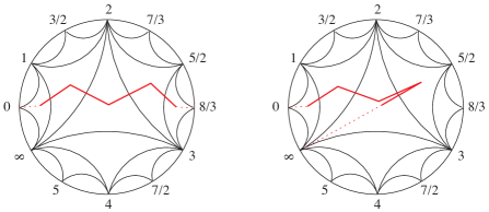
Figure 13. Two paths of triangles. The first gives a triangulation of $L(8,3)$ containing the torus knots $K(1,0)$ and $K(2,1)$, and other torus knots equivalent to these. The second path is not injective and gives a triangulation of $L(1,0)$ containing $K(5,2)$, i.e. the $(5,2)$ torus knot in $S^{3}$. Both triangulations contain $5-3=2$ tetrahedra.

Let then $\lambda(\ell,m,p,q)$ be the length of the shortest path of triangles from $0/1$ to $p/q$ which contains $\ell/m$. By what just said, we have:

$$c\big{(}L(p,q),K(\ell,m)\big{)}\leqslant\max\big{\{}\lambda(\ell,m,p,q)-3,0\big{\}}.$$

It was conjectured in [32] that every $L(p,q)=\big{(}L(p,q),\emptyset\big{)}$ with $c\neq 0$ has a minimal triangulation which is layered, namely that $c\big{(}L(p,q)\big{)}=\max\big{\{}\lambda(p,q)-3,0\big{\}}$, where $\lambda(p,q)$ is the length of the shortest path of triangles from $0/1$ to $p/q$. We now propose the following extension:

Conjecture 6.4.

The complexity of a $(0,1,2)$-irreducible torus knot in a lens space is

$$c\big{(}L(p,q),K(\ell,m)\big{)}=\max\big{\{}\lambda(\ell,m,p,q)-3,0\big{\}}.$$

As the census in Table 10 shows, the conjecture holds for complexity up to $2$.

6.4. Non-hyperbolic knots and links

The non-hyperbolic knots and links up to complexity 2, and those having complexity 3 contained in $S^{3}$, are described in Table 10. They are all torus links in lens spaces, except for a knot in the elliptic Seifert space $S^{3}/{Q_{8}}$, whose exterior is the twisted interval bundle over the Klein bottle. This pair is pictured in Figure 14.

Note that $L(7,2)$ is the only lens space in the table not admitting a symmetry switching the two cores of the Heegaard solid tori, and that both these cores appear in the list.

$c$	type	space	description of knot or link
0	knot	$S^{3}$	$K(1,0)=$ unknot
0	knot	${\mathbb{P}}^{3}$	$K(1,0)=$ core of Heegaard torus
0	knot	$L(3,1)$	$K(1,0)=$ core of Heegaard torus
1	knot	$S^{3}$	$K(3,2)=$ trefoil
1	link	$S^{3}$	$K(2,2)=$ Hopf link
1	knot	$L(4,1)$	$K(1,0)=$ core of Heegaard torus
1	knot	$L(5,2)$	$K(1,0)=$ core of Heegaard torus
2	knot	$S^{3}$	$K(5,2)=5_{1}$ [43]
2	knot	$L(5,1)$	$K(1,0)=$ core of Heegaard torus
2	knot	$L(7,2)$	$K(1,0)=$ core of one Heegaard torus
2	knot	$L(7,2)$	$K(3,1)=$ core of other Heegaard torus
2	knot	$L(8,3)$	$K(1,0)=$ core of Heegaard torus
2	knot	$L(5,1)$	$K(2,1)$
2	knot	$L(7,2)$	$K(2,1)$
2	knot	$L(8,3)$	$K(2,1)$
2	knot	$S^{2}\times S^{1}$	$K(3,1)$
2	knot	$L(3,1)$	$K(3,2)$
2	knot	${\mathbb{P}}^{3}$	$K(4,1)$
2	link	${\mathbb{P}}^{3}$	$K(2,2)=$ union of cores of Heegaard tori
2	knot	$S^{3}/Q_{8}$	singular fibre of $\big{(}S^{2};(2,-1),(2,1),(2,1)\big{)}$
3	knot	$S^{3}$	$K(4,3)=8_{19}$ [43]
3	knot	$S^{3}$	$K(5,3)=10_{123}$ [43]
3	knot	$S^{3}$	$K(7,2)=7_{1}$ [43]
3	link	$S^{3}$	$K(4,2)=4^{2}_{1}$ [43]

Table 10. Information on non-hyperbolic knots and links. In complexity 3 only knots and links in the 3-sphere are described. In the description of torus knots, we set $S^{3}=L(1,0)$, ${\mathbb{P}}^{3}=L(2,1)$, and $S^{2}\times S^{1}=L(0,1)$.

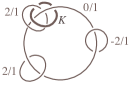
Figure 14. A surgery presentation of the pair $(M,K)$ where $M=S^{3}/Q_{8}=\big{(}S^{2};(2,-1),(2,1),(2,1)\big{)}$ and $K$ is a singular fibre of the fibration.

6.5. $\theta$-graphs with Klein bottles

In complexity 5 we have only investigated pairs $(M,G)$ where $G$ is non-empty and all its components have vertices. As mentioned above, we have found here 5 very interesting pairs, where $G$ is a $\theta$-graph and the pair $(M,G)$ is $(0,1,2)$-irreducible, but non-hyperbolic since $M\setminus G$ contains an embedded Klein bottle, so it is not atoroidal.

Proposition 6.5.

There are five $(0,1,2)$-irreducible non-hyperbolic pairs $(M,G)$ such that $c(M,G)=5$ and $G$ has no knot component. They are described as follows:

• Let ${\mathbb{K}}$ be the twisted interval bundle over the Klein bottle.

• Let $({\mathbb{T}},\theta)$ be the solid torus with the embedded $\theta$-graph shown in Figure 15.

• Then $(M,G)$ is obtained by gluing ${\mathbb{K}}$ to $({\mathbb{T}},\theta)$ so that $M$ is one of the manifolds $S^{2}\times S^{1}$, $S^{3}/{Q_{8}}$, $L(8,3)$, $L(4,1)$, or $\mathbb{RP}^{3}\#\mathbb{RP}^{3}$.

Figure 15. The theta graph $\theta$ in the solid torus ${\mathbb{T}}$.

This result was proved as follows. We first analyzed the triangulations of the $5$ pairs $(M,G)$ produced by our Haskell code on which Orb failed to construct a hyperbolic structure. This allowed us to show that the $5$ pairs are those described in points (i)-(iii) of the statement, whence to see that they are not hyperbolic. We then proved that they are indeed (0,1,2)-irreducible by classical topological techniques, the key point being that a compressing disc of $({\mathbb{T}},\theta)$ must intersect $\theta$ in at least two points.

Here are the details of the argument. Suppose there is a sphere $S$ intersecting $G$ transversely in at most $2$ points, and isotope $S$ to minimize its intersection with $\partial{\mathbb{T}}$. Now consider an innermost disc $D$ on $S$ bounded by a simple closed curve in $S\cap\partial{\mathbb{T}}$. Since there is no compressing disc in ${\mathbb{K}}$, such a disc must be a compressing disc in ${\mathbb{T}}$, so it must intersect $\theta$ at least twice. But if $S\cap\partial{\mathbb{T}}\neq\emptyset$ then there are at least two innermost discs on $S$, whence $S\cap G$ contains at least 4 points, which is impossible. This shows that $S$ is disjoint from $\partial{\mathbb{T}}$, so it is contained either in ${\mathbb{K}}$ or in ${\mathbb{T}}$. However ${\mathbb{K}}$ is irreducible, and $({\mathbb{T}},\theta)$ is $(0,1,2)$-irreducible (in fact, it is easy to see that it is hyperbolic with parabolic meridians). Therefore $S$ must bound a trivial ball in $(M,G)$.

7. Figures

This section contains pictures of the hyperbolic graphs up to complexity 4, given in the form of a surgery description when the underlying space is not $S^{3}$. For each graph, we give the name and the volume of the hyperbolic structure with parabolic meridians.

The figures were produced using Orb [19] and the census of knotted graphs in [5]. Most of the graphs in $S^{3}$ occurred in [5]; the graphs not in $S^{3}$ generally arose as Dehn surgeries on knot components of disconnected graphs in [5]. There were a couple of remaining examples which were constructed by hand. In all cases, we used Orb to identify the graphs by matching triangulations.

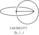
Figure 16. Complexity 1.

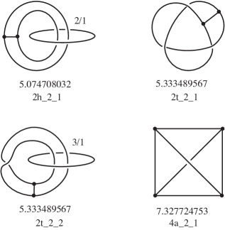
Figure 17. Complexity 2.

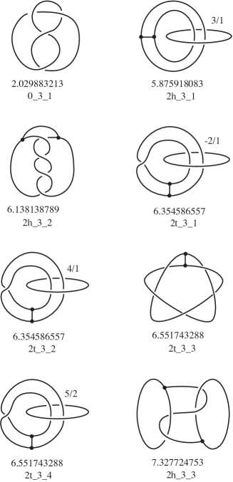
Figure 18. Complexity 3.

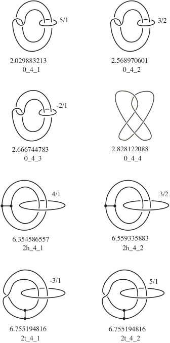
Figure 19. Complexity 4, part 1 of 4.

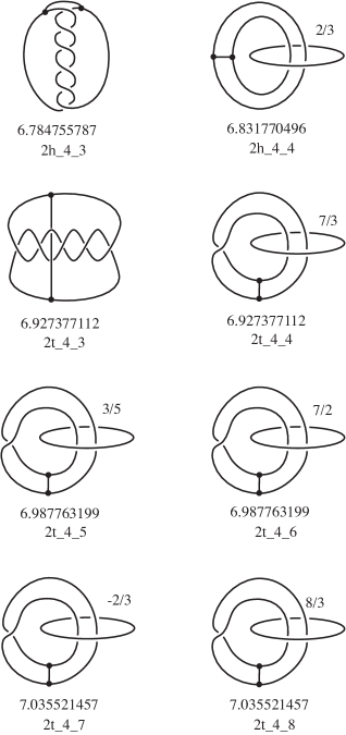
Figure 20. Complexity 4, part 2 of 4.

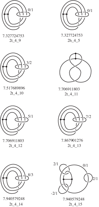
Figure 21. Complexity 4, part 3 of 4.

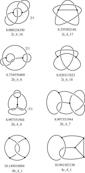
Figure 22. Complexity 4, part 4 of 4.

References

- [1] M. Boileau, B. Leeb, J. Porti, Geometrization of -dimensional orbifolds, Ann. of Math. 162 (2005), 195-290.
- [2] P. J. Callahan, M. V. Hildebrand, J. R. Weeks, A census of cusped hyperbolic -manifolds, Math. Comp. 68 (1999), 321-332.
- [3] C. Cao, G. Meyerhoff, The orientable cusped hyperbolic -manifolds of minimum volume, Invent. Math. 146 (2001), 451-478.
- [4] A. Casson, “Geo”, A computer program for geometrizing -manifolds, available from computop.org.
- [5] M. Chiodo, D. Heard, C. Hodgson, J. Saunderson, N. Sheridan, Enumeration and classification of knotted graphs in , in preparation.
- [6] J. Conway, An enumeration of knots and links, and some of their algebraic properties, in: Computational Problems in Abstract Algebra (Proc. Conf., Oxford, 1967), 329-358, Pergamon, Oxford, 1970.
- [7] D. Cooper, C. Hodgson, S. Kerckhoff, “Three-Dimensional Orbifolds and Cone Manifolds”, Mathematical Society of Japan Memoirs, Vol. 5, Tokyo, 2000.
- [8] D. Coulson, O. Goodman, C. Hodgson, W. Neumann, Computing arithmetic invariants of -manifolds, Experiment. Math. 9 (2000), 127-152.
- [9] D. B. A. Epstein, R. C. Penner, Euclidean decompositions of noncompact hyperbolic manifolds, J. Differential Geom. 27 (1988), 67-80.
- [10] E. Flapan, “When Topology Meets Chemistry. A topological look at molecular chirality”, Cambridge University Press, Cambridge, 2000.
- [11] R. Frigerio, B. Martelli, C. Petronio, Small hyperbolic -manifolds with geodesic boundary, Experiment. Math. 13 (2004), 171-184.
- [12] R. Frigerio, C. Petronio, Construction and recognition of hyperbolic -manifolds with geodesic boundary, Trans. Amer. Math. Soc. 356 (2004), 3243-3282.
- [13] M. Fujii, Hyperbolic -manifolds with totally geodesic boundary which are decomposed into hyperbolic truncated tetrahedra, Tokyo J. Math. 13 (1990), 353-373.
- [14] D. Gabai, R. Meyerhoff, P. Milley, Mom technology and volumes of hyperbolic -manifolds, arXiv:math.GT/0606072.
- [15] by same author, Minimum volume cusped hyperbolic three-manifolds, arXiv:math.GT/0705.4325.
- [16] F. W. Gehring, G. J. Martin, Minimal co-volume hyperbolic lattices I: the spherical points of a Kleinian group, Ann. of Math., to appear.
- [17] O. Goodman, “Snap”, A computer program for studying arithmetic invariants of hyperbolic -manifolds, available from www.ms.unimelb.edu.au/~snap and sourceforge.net/projects/snap-pari.
- [18] “Haskell”, An advanced purely functional programming language, available from www.haskell.org.
- [19] D. Heard, “Orb”, The computer program for finding hyperbolic structures on hyperbolic 3-orbifolds and -manifolds, available from www.ms.unimelb.edu.au/~snap/orb.html.
- [20] by same author, Computation of hyperbolic structures on -dimensional orbifolds, PhD thesis, University of Melbourne, 2005, www.ms.unimelb.edu.au/~snap/DHeard-PhD.pdf.
- [21] J. Hoste, M. Thistlethwaite, J. Weeks, The first 1,701,936 knots. Math. Intelligencer 20 (1998), no. 4, 33-48.
- [22] W. Jaco, J. H. Rubinstein, Layered triangulations of -manifolds, arXiv:math.GT/0603601 .
- [23] M. Kapovich, “Hyperbolic Manifolds and Discrete Groups”, Progress in Mathematics, Vol. 183, Birkhäuser Inc., Boston, MA, 2001.
- [24] S. Kojima, Polyhedral decomposition of hyperbolic manifolds with boundary, Proc. Work. Pure Math. 10 (1990), 37-57.
- [25] by same author, Polyhedral decomposition of hyperbolic -manifolds with totally geodesic boundary, In: “Aspects of low-dimensional manifolds”, Adv. Stud. Pure Math. Vol. 20, Kinokuniya, Tokyo, 1992, pp. 93-112.
- [26] S. Kojima, Y. Miyamoto, The smallest hyperbolic -manifolds with totally geodesic boundary, J. Differential Geom. 34 (1991), 175-192.
- [27] R. Litherland, A table of all prime theta-curves in up to crossings, letter, 1989.
- [28] C. Maclachlan, A. Reid, “The Arithmetic of Hyperbolic 3-Manifolds”, Springer-Verlag, New York, 2003.
- [29] T. H. Marshall, G. J. Martin, Minimal co-volume hyperbolic lattices, II: simple torsion in Kleinian groups, preprint.
- [30] B. Martelli, C. Petronio, -manifolds having complexity at most , Experiment. Math. 10 (2001), 207-237.
- [31] by same author, Complexity of geometric -manifolds, Geom. Dedicata 108 (2004), 15-69.
- [32] S. V. Matveev, Complexity theory of three-dimensional manifolds, Acta Appl. Math. 19 (1990), 101-130.
- [33] by same author, Transformations of special spines, and the Zeeman conjecture (Russian), Izv. Akad. Nauk SSSR Ser. Mat. 51 (1987), 1104-1116, 1119. (English translation: Math. USSR-Izv. 31 (1988), 423-434.)
- [34] by same author, “Algorithmic Topology and Classification of 3-Manifolds”, Algorithms and Computation in Mathematics, Vol. 9, Springer-Verlag, Berlin, 2003.
- [35] by same author, Tabulation of three-dimensional manifolds, Russ. Math. Surv. 60 (2005), 673-698.
- [36] Y. Miyamoto, Volumes of hyperbolic manifolds with geodesic boundary, Topology 33 (1994), 613-629.
- [37] J. Morgan, On Thurston’s uniformization theorem for three-dimensional manifolds, In: “The Smith Conjecture” (New York, 1979), Pure Appl. Math. Vol. 112, Academic Press, Orlando, FL, 1984, pp. 37-125.
- [38] H. Moriuchi, An enumeration of theta-curves with up to seven crossings, In: Proceedings of the East Asian School of Knots, Links, and Related topics, 2004, Seoul, Korea, pp. 171-185, knot.kaist.ac.kr/2004/proceedings/MORIUCHI.pdf.
- [39] by same author, A table of handcuff graphs with up to seven crossings, OCAMI Studies Vol. 1, Knot Theory for Scientific Objects (2007), www.omup.jp/modules/papers/knot/chap15.pdf.
- [40] C. Petronio, Spherical splitting of -orbifolds, Math. Proc. Cambridge Philos. Soc. 142 (2007), 269-287.
- [41] by same author, Complexity of -orbifolds, Topology Appl. 153 (2006), 1658-1681.
- [42] R. Piergallini, Standard moves for standard polyhedra and spines, Rend. Circ. Mat. Palermo (2) Suppl. 18 (1988), 391-414.
- [43] D. Rolfsen, “Knots and Links”, Publish or Perish, Berkeley, California, 1976.
- [44] C. Rourke, B. Sanderson, “Introduction to Piecewise Linear Topology”, Ergebn. der Math. Vol. 69, Springer-Verlag, New York-Heidelberg, 1972.
- [45] J. Simon, A topological approach to the stereochemistry of nonrigid molecules, Graph theory and topology in chemistry (Athens, Ga., 1987), 43–75, Stud. Phys. Theoret. Chem., 51, Elsevier, Amsterdam, 1987.
- [46] W. P. Thurston, “Geometry and Topology of 3-Manifolds”, mimeographed notes, Princeton University, 1979, available from msri.org/publications/books/gt3m/.
- [47] by same author, Hyperbolic geometry and -manifolds, In: “Low-Dimensional Topology” (Bangor, 1979), London Math. Soc. Lecture Note Ser. Vol. 48, Cambridge University Press, Cambridge, New York, 1982, pp. 9-25.
- [48] by same author, “Three-dimensional geometry and topology”, Vol. 1, Princeton University Press, 1997.
- [49] J. L. Tollefson, Involutions of sufficiently large -manifolds, Topology 20 (1981), 323-352.
- [50] A. Ushijima, The tilt formula for generalized simplices in hyperbolic space, Discrete Comput. Geom. 28 (2002), 19-27.
- [51] J. R. Weeks, “SnapPea”, The hyperbolic structures computer program, available from www.geometrygames.org.
- [52] by same author, Convex hulls and isometries of cusped hyperbolic -manifolds, Topology Appl. 52 (1993), 127-149.