We analyze a controllable generation of maximally entangled mixed states of a circuit containing two-coupled superconducting charge qubits. Each qubit is based on a Cooper pair box connected to a reservoir electrode through a Josephson junction. Illustrative variational calculations were performed to demonstrate the effect on the two-qubits entanglement. At sufficiently deviation between the Josephson energies of the qubits and/or strong coupling regime, maximally entangled mixed states at certain instances of time is synthesized. We show that entanglement has an interesting subsequent time evolution, including the sudden death effect. This enables us to completely characterize the phenomenon of entanglement sharing in the coupling of two superconducting charge qubits, a system of both theoretical and experimental interest.

1 Introduction

There have been remarkable advances in the quest to build a superconductor-based quantum information processor in recent years [1, 2] and one of the greatest scientific and engineering challenges of this decade is the realization of a quantum computer. In this context, a solid-state system is highly desirable because of its compactness, scalability and compatibility with existing semiconductor technology. One of the physical realizations of a solid-state qubit is provided by a Cooper pair box which is a small superconducting island connected to a large superconducting electrode, a reservoir, through a Josephson junction [3]. Superconducting charge qubits (Cooper pair boxes) are a promising technology for the realization of quantum computation on a large scale [4, 5, 6, 7, 8].

Using simultaneous measurement and state tomography, entanglement between two solid-state qubits has been demonstrated [9]. The results demonstrate a high degree of unitary control of the system, indicating that larger implementations are within reach. These results are promising for future solid-state quantum computing. For conventional fault-tolerant quantum computing, the quantum states should have a high level of purity, preferably being as close to a pure state as possible. When the qubit is coupled to an environment it is subject to decoherence, which will typically result in a completely mixed state [10]. However, a qubit initially in a completely mixed state can be purified by measurement. Therefore, it is desirable on both fundamental and practical grounds to study maximin entangled state generation and entanglement dynamics in a time-dependent sense. One of the next major steps towards building a Josephson junction quantum computer prototype will be the demonstration of controllable coupling between the qubits. At this end, it seems that a quantitative link between the degree of disentanglement and the amount of the energy transferred between the system of interest and its environment is still missing. Investigation of entanglement control in such systems would therefore be an important contribution to the present suite of experimental controls.

In recent years quantum entanglement has found many exciting applications that have considerable bearing on the emerging fields of quantum information and quantum computing [11, 12, 13, 14, 15]. Moreover, besides this fundamental aspect, the interest in entangled states has been recently renewed because their properties lie at the heart of many potential applications. The generation and reconstruction of quantum states were extensively studied in the past theoretically and experimentally [16, 17, 18, 19, 20]. More fundamentally, decoherence processes due to the interaction with internal or external noises and entanglement decay in a time-dependent sense have been studied in many distinct cases [12, 21, 23, 24, 25, 26, 27]. More recently, Almeida et al. [14] have devised an elegantly clean way to confirm the existence of so-called entanglement sudden death, that is, entanglement terminates completely after a finite interval, without a smoothly diminishing long-time tail.

This paper examines the generation of maximally entangled mixed state of two-coupled Josephson charge qubits using a common pulse gate. We present various examples in order to monitor different regimes of synthizing the maximally entangled mixed states and entanglement dynamics. In principle, by proper adjustment of the initial state parameters, we can always find suitable values of characteristic energies of the Cooper pairs and coupling energy which can be used to suppress the decay of entanglement. This analysis is carried out with generalized time-dependent density matrix, yielding a generalized dynamical two-qubit model. As we are going to show, we may take this advantage to increase time intervals for maximally entangled states caused by the strong coupling regime.

This paper is organized as follows: In Sec. 2, we will describe the Hamiltonian of the system of interest, and obtain the explicit analytical solution of the master equation describing the dynamics of two qubits in the presence of phase decoherence. In Sec. 3, by calculating the occupation probabilities of the two qubits, we show that it is possible to generate the maximally entangled mixed states of the system in different situations. In Sec. 4, we discuss the entanglement of the system by virtue of the concurrence in the absence or presence of the decoherence. Finally, Sec. 5 presents the conclusions and an outlook.

Figure 1: Illustration of two capacitively coupled Josephson charge qubits. The circuite consists of two charge qubits that are coupled by an on-chip capacitor $C_{m}$ [6, 28].

2 Two coupled charge qubits

Here, we briefly discuss the general formalism to characterize the dynamics of two-coupled superconducting charge qubits (Cooper pair boxes connected to a reservoir electrode through a Josephson junction). For a more detailed discussion we refer the reader to Ref. [6, 30]. We consider two charge qubits and couple them by means of a miniature on-chip capacitor. The read-out of each qubit, in this case, is done similar to the single qubit read-out and connect a probe electrode to each qubit. External controls that we have in the circuit are the dc probe voltages $V_{b_{1}}$ and $V_{b_{2}}$, $d_{c}$ gate voltages $V_{g_{1}}$ and $V_{g_{2}}$, and pulse gate voltage $V_{p}$ (see figure 1). The information on the final states of the qubits after manipulation comes from the pulse-induced currents measured in the probes. By doing routine current– voltage–gate voltage measurements, we can estimate the capacitances. We then perform state manipulation and demonstrate qubit–qubit interaction. The Hamiltonian of the system in the charge representation can be written as

$$\hat{H}=\hbar\sum_{n_{1}=0}^{\infty}\sum_{n_{2}=0}^{\infty}\eta_{1}(n_{1},n_{2})\widehat{S}_{11}-\frac{E_{J_{1}}}{2}\left(\widehat{S}_{12}+\widehat{S}_{34}\right)-\frac{E_{J_{2}}}{2}\left(\widehat{S}_{13}+\widehat{S}_{24}\right),$$ (1)

where $\widehat{S}_{11}=|n_{1},n_{2}\rangle\langle n_{1},n_{2}|,$ $\widehat{S}_{12}=|n_{1},n_{2}\rangle\langle n_{1}+1,n_{2}|,$ $\widehat{S}_{13}=|n_{1},n_{2}\rangle\langle n_{1},n_{2}+1|,$ $\widehat{S}_{34}=|n_{1},n_{2}+1\rangle\langle n_{1}+1,n_{2}+1|,$ and $\widehat{S}_{24}=|n_{1}+1,n_{2}\rangle\langle n_{1}+1,n_{2}+1|.$ The parameter $\eta_{1}(n_{1},n_{2})=E_{c_{1}}\left(n_{g_{1}}-n_{1}\right)^{2}+E_{c_{2}}\left(n_{g_{2}}-n_{2}\right)^{2}+E_{m}\left(n_{g_{1}}-n_{1}\right)\left(n_{g_{2}}-n_{2}\right).$ Here, $n_{1}$ and $n_{2}$ ($n_{1},n_{2}=0,\pm 1,\pm 2,...$) are the numbers of excess Cooper pairs in the first and the second Cooper pair boxes, and $n_{g_{1,2}}=(C_{g_{1,2}}V_{g_{1,2}}+C_{p}V_{p})/2e$ are the normalized charges induced on the corresponding qubit by the $d_{c}$ and pulse gate electrodes. The eigenenergies, $E_{k}$ $(k=0,1,2,...$), of the Hamiltonian (1) form $2e$-periodic energy bands corresponding to the ground ($k=0$), first excited ($k=1$), etc. states of the system. $E_{c_{1}}$, $E_{c_{2}}$ and $E_{m}$ give the characteristic energies of Cooper pair of the first qubit, Cooper pair charging energy of the second qubit and the coupling energy, respectively.

$$E_{c1,2} = \frac{4e^{2}C_{\varepsilon 2,1}}{2(C_{\varepsilon 1}C_{\varepsilon 2}-C_{m}^{2})},$$

$$E_{m} = \frac{4e^{2}C_{m}}{C_{\varepsilon 1}C_{\varepsilon 2}-C_{m}^{2}},$$ (2)

where $C_{\varepsilon_{1,2}}$ are the sum of all capacitances connected to the corresponding Cooper pair box including the coupling capacitance $C_{m}$ and $e$ is the electron charge.

If the circuit is fabricated to have the following relation between the characteristic energies: $E_{J_{1,2}}\sim$ $E_{m}<E_{c_{1,2}}$, then one can use a four-level approximation for the description of the system ($|00\rangle,|01\rangle,|01\rangle$ and $|11\rangle$) around $n_{g_{1}}=n_{g_{2}}=0.5$ while other charge states are separated by large energy gaps. In this basis, the two charge qubits system behaves as a single four-level system which can be used as a new basis for the Hamiltonian (1).

The time evolution of the system density operator $\hat{\rho}(t)$ can be written as [31, 32, 33]

$$\frac{d}{dt}\hat{\rho}(t)=-\frac{i}{\hbar}[\hat{H},\hat{\rho}]-\frac{\gamma}{2\hbar^{2}}[\hat{H},[\hat{H},\hat{\rho}]],$$ (3)

where $\gamma$ is the phase decoherence rate. Equation (3) reduces to the ordinary von Neumann equation for the density operator in the limit $\gamma\rightarrow 0.$ The equation with the similar form has been proposed to describe the intrinsic decoherence [34]. Under Markov approximations the  solution of the master equation can be expressed in terms of Kraus operators [35] as follows

$$\hat{\rho}(t) = \sum_{m=0}^{\infty}\frac{\left(\gamma t\right)^{m}}{m!}\hat{H}^{m}\exp\left(-i\hat{H}t\right)\exp\left(-\frac{\gamma t}{2}\hat{H}^{2}\right)\hat{\rho}(0)\exp\left(-\frac{\gamma t}{2}\hat{H}^{2}\right)\exp\left(i\hat{H}t\right)\hat{H}^{m}$$ (4)

$$= \sum_{m=0}^{\infty}\frac{\left(\gamma t\right)^{m}}{m!}\hat{M}^{m}(t)\hat{\rho}(0)\hat{M}^{\dagger m}(t),\qquad\qquad\qquad$$

where $\hat{\rho}(0)$ is the density operator of the initial state of the system and $\hat{M}^{m}$ are the Kraus operators which completely describe the reduced dynamics of the qubits system,

$$\hat{M}^{m}=\hat{H}^{m}\exp(-i\hat{H}t)\exp\left(-\frac{\gamma t}{2}\hat{H}^{2}\right).$$ (5)

Equation (4) can also be written as

$$\rho(t) = \exp\left(-i\hat{H}t\right)\exp\left(-\frac{\gamma t}{2}\hat{H}^{2}\right)\{e^{\hat{S}_{M}t}\hat{\rho}(0)\}\exp\left(-\frac{\gamma t}{2}\hat{H}^{2}\right)\exp\left(i\hat{H}t\right)$$

$$= \rho_{ij,lk}(t)|ij\rangle\langle lk|.$$

We define the superoperator $\hat{S}_{M}\hat{\rho}(0)=\gamma\hat{H}\hat{\rho}(0)\hat{H}$ and choose arbitrary initial state of the two charge qubits. The notation $|ij\rangle=|i\rangle_{1}\otimes|j\rangle_{2},$ is used, where $|0\rangle_{1(2)}$ and $|0\rangle_{1(2)}$ are the basis states of the first (second) qubits and $\rho_{ij,lk}(t)=\langle ij|\rho(t)|lk\rangle$ corresponds the diagonal ($ij=lk$) and off-diagonal ($ij\neq lk)$ elements of the final state density matrix $\rho(t).$ From here on, for tractability of notation and without loss of generality, we denote by $\rho_{ij}(t)=\rho_{ij,ij}(t),$ the probability of finding the two-coupled charge qubits in the state $|ij\rangle.$

3 Creation of maximally entangled mixed states

We now apply the above results to study the time evolution of the occupation probabilities with different values of the system parameters. In pure-state case, there has been considerable debate over the entanglement properties of certain types of states [11]. In this paper, we are interested in the case in which the final state of the coupled charge qubits $\rho(t)$ is a maximally entangled mixed state [19].

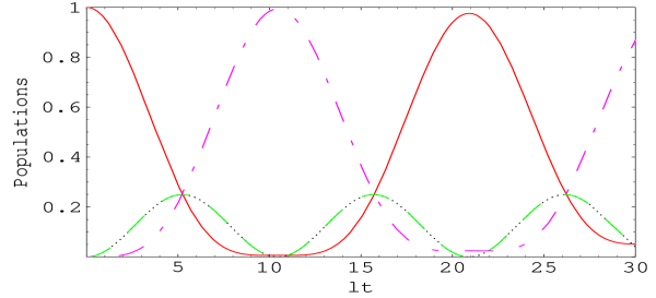
Figure 2: The time evolution of the occupation probabilities $\rho_{ij}(t),$ where $\rho_{00}(t)$ (solid curve), $\rho_{01}(t)$ (dashed curve), $\rho_{10}(t)$ (dot-dashed curve) and $\rho_{11}(t)$ (dotted curve). The initial state of the two-charge qubits is assumed to be $\rho(0)=|00\rangle\langle 00|$ and the parameters used in these figures are $E_{J1}=E_{J2}=30$ and $E_{m}=6.$

Nakamura et al. [36] investigated the temporal behavior of a Cooper-pair box driven by a strong microwave field and observed the Rabi oscillations with multi-photon exchanges between the two-level system and the microwave field. Here, the occupation probabilities as functions of  the scaled time $\lambda t$ are schematically shown in Fig. 2. Note that the populations of the four states exist but $\rho_{00}(t)$ as well as $\rho_{10}(t)$ oscillate between $0$ and $1,$ while $\rho_{01}(t)$ and $\rho_{11}(t)$ oscillate with smaller amplitudes. It should be noted that the occupation probabilities results are drastically different when we consider different initial state settings. To analyze the effect of the system parameters on the occupation probabilities for the present system we consider two different cases. One when the the Josephson energies of Cooper pair are different while the second case is the strong interaction regime. This will be seen in figure 3 and figure 4. As an example of the creation of the two-particle maximally entangled state is shown in Fig. 3. The results of this figure are obtained for parameters $E_{J1}=30\mu$eV$,E_{J2}=5\mu$eV and $E_{m}=6\mu$eV. The way to determine experimentally the qubits’ Josephson energies $E_{J1}$ and $E_{J2}$ has been described in Ref. [30]

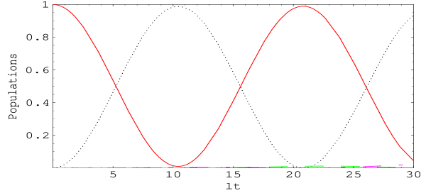
Figure 3: The same as figure 1, but $E_{J1}=30\mu eV,E_{J2}=5\mu$eV and $E_{m}=6\mu eV.$

If the system starts from excited state, $\rho(0)=\left|0,0\right\rangle\left\langle 0,0\right|,$ we see that the occupation probabilities of the intermediate states tend to zero at any instant of time and the Cooper pair system oscillate only between excited and ground states. If the environment is switched off, i.e. $\gamma$ tends to zero, and using equation (2), at some instant times $\tau\simeq\frac{5n}{\lambda},(n=1,2,3,...)$, we can obtain analytically the values of the diagonal and off-diagonal elements of the density matrix as $\rho_{00,00}(t)=\rho_{11,11}(t)=0.5$ and $\rho_{00,11}(t)=\rho_{11,00}(t)=\zeta\neq 0,$ otherwise  $\rho_{ij,lk}(t)=0.$ Which means that, the final state takes the form

$$\hat{\rho}(t)=\frac{1}{2}\left|0,0\right\rangle\left\langle 0,0\right|+\zeta(\left|0,0\right\rangle\left\langle 1,1\right|+\left|1,1\right\rangle\left\langle 0,0\right|)+\frac{1}{2}\left|1,1\right\rangle\left\langle 1,1\right|,$$ (7)

i.e. the final state (7) becomes a maximally entangled mixed state [19]. This entangled state corresponds to the half-probability peaks in figure 3 ($\zeta=0.13)$. Depending on whether Josephson energy of the first qubit is smaller or larger than the Josephson energy of the second qubit, the maximally entangled states are created. Similarly, depending on the coupling energy the maximally entangled state is characterized as having short or long correlation time. Given enough time, the system will therefore reaches a state where both excited and ground states have equal occupation probabilities i.e. the coupled-qubit system evolves to the maximally entangled mixed state at the times given by

$$\lambda t=\frac{n\pi}{\sqrt{(E_{J1}+E_{J2})^{2}+E_{m}^{2}/4}-\sqrt{(E_{J1}-E_{J2})^{2}+E_{m}^{2}/4}},n=\pm 1,\pm 2,\pm 3,....$$ (8)

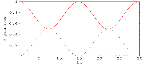
Figure 4: The same as figure 1, but $E_{J1}=30\mu eV,E_{J2}=1\mu$eV and $E_{m}=60\mu eV.$

We turn our attention to consider the case in which both characteristic energies have different values taking into account the effect of the coupling energy. For this reason we have plotted the function $\rho_{ij}(t)$ against the scaled time $\lambda t$ in figures (4). To make a comparison between this case and the previous one we have to take the values of the other parameters similar to that of the previous case. In this case and providing the characteristic energies $E_{J1}=30\mu$eV, and $E_{J2}=6\mu eV,$ we find that the function reduces its value to be around $\approx 1$ and $0.5$ for the excited state while the ground state probability oscillates between $0$ and $0.5$. Furthermore, we realize there is a long period of the interaction time in which the probability of the excited state equals the ground state probability, with perfect symmetric fluctuation pattern around $0.5$, see figure (4). Which means that, with these setting, we obtained long lived maximally entangled mixed state (in this case $\zeta=0.19)$. In the meantime if we exchange the values of the characteristic energies, we observe there is no big change in the figure shape, except some decreases in the fluctuations number. It is to be noted that the maximally entangled state in this case is lived longer compared with significantly short time in the previous case (see figures 3 and 4).

One might now raise the following notes: taking a strong coupling regime where the coupling energy is strong enough, one can obtains maximally entangled mixed states at some instant times in a periodical manner. But when the coupling energy between the two qubits is weak, the period becomes shorter. Also, if the deviation between the Josephson energies is substantially large, the maximally entangled states can be generated. It is worth noting that when the coupling energy tends to zero, our model becomes similar to that of a beam splitter model. In such a case, we cannot obtain maximally entangled states.

The above discussion clearly shows that the maximally entangled state generation of the two charge qubits depends on both the time evolution, Josephson energies of both charge qubits and coupling energy. The considerations of experimental observability of the entangling power discussed in [3] are valid in the context of the present work.

4 Entanglement

Having established the existence of maximally entangled states $\rho(t),$ in section 3, now we try to answer the following question: how does the entanglement of the two charge qubits system evolve? To answer this question, one first needs a formal definition of entanglement. Currently a variety of measures are known for quantifying the degree of entanglement in a bipartite system [37, 38, 39, 40, 41, 42, 43]. A convenient measure of entanglement for a two-qubit state $\rho(t)$ is the concurrence $C_{\rho}\left(t\right),$ given by

$$C_{\rho}\left(t\right)=\max\left\{0,\lambda_{1}-\lambda_{2}-\lambda_{3}-\lambda_{4}\right\},$$ (9)

where $\lambda_{1}\geq\lambda_{2}\geq\lambda_{3}\geq\lambda_{4}.$ We denote by $\lambda_{i}$ the square roots of the eigenvalues of $\rho\left(\sigma_{y}\otimes\sigma_{y}\right)\left(\rho\right)^{\ast}\left(\sigma_{y}\otimes\sigma_{y}\right),$ here $\sigma_{y}$ is the second Pauli matrix and the conjugation occurs in the computational basis $(|00\rangle$, $|01\rangle$, $|10\rangle$, $|11\rangle)$. $C_{\rho}\left(t\right)$ quantifies the amount of quantum correlation that is present in the system and can assume values between $0$ (only classical correlations) and $1$ (maximal entanglement).

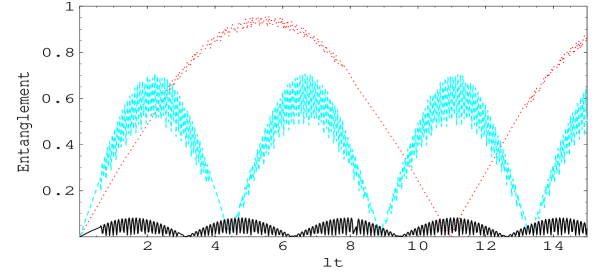
Figure 5: The time evolution of the concurrence as a function of the scaled time $\lambda t.$ The parameters are E${}_{\emph{J1}}$=30$\mu$eV ,  E${}_{\emph{J2}}$=2$\mu$eV,  $\gamma=0$ and different values of the coupling energy, where E_m=200$\mu$eV (dotted curve), E_m=60$\mu$eV (dashed curve) and E_m=5$\mu$eV (solid curve). Regions of the entanglement sudden death are painted in gray.

In figure 5, we plot the concurrence as a function of the scaled time assuming that the two-coupled superconducting charge qubits start from their excited states. The maximum value of the entanglement decreases as the coupling energy is decreased. As time goes on, the entanglement reaches zero value in a periodic way, this period decreases as the coupling energy decreases. In the uncoupled situation each qubit oscillates with its own frequency and $C_{\rho}\left(t\right)=0$. It is interesting to note that, the maximum entanglement is achieved at specific choices of the interaction time i.e. the entanglement content corresponding to specific choices of the interaction time and large values of the coupling energy. We therefore consider the question of how the coupling energy affect the entanglement of system. In relation to that discussion, it is useful to examine the effect of the characteristic energies with fixing the coupling energy of the two charge qubits that change their state during the transition. That criterion is related to, but clearly distinct from, the question of quantifying how maximum a quantum state is. Also, as can be seen from the graphs figures 3 and 5, the entanglement vanishes at the time at which the population of the symmetric state is maximal.

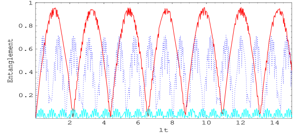
Figure 6: The same as figure 4 but E${}_{\emph{J2}}$=5$\mu$eV.

Put differently, with a small difference between the characteristic energies of the Cooper pairs (Josephson energy of the second qubit, E${}_{\emph{J2}}$=5$\mu$eV) and still kept the parameter values of figure 5, we show that the entanglement features are visibly worsened, as in this regime oscillations are faster than the previous case (see figure 6) in which big difference between the characteristic energies of both qubits are considered. One has still zero entanglement due to the time development, but with a short period of the interaction time which is roughly given by $\lambda t\approx\frac{2n\pi}{3},(n=1,2,3,...)$. Similar to the previous case, one will have a very small amount of entanglement when the coupling energy decreases and this amount disappear completely when the coupling energy decreases further. Indeed, the comparison of plots figure 5 and figure 6, demonstrates that the entanglement in both cases has somewhat similar behavior corresponding to different values of coupling energy. The deviation value of the Josephson energies of the Cooper pairs effect on the entanglement is particularly pronounced as this deviation is much bigger.

Conventionally, maximally entangled state emerge from the coupling of the two qubits by a small island overlapping both Cooper pair boxes, i.e. two-coupled superconducting charge qubits. As such, the phenomenon is the result of many-particle dynamics, often described by a simple interaction model. In the single-qubit case novel features appear which are due to the coherent microscopic dynamics. Our study allows us to identify the dependence of these features on different parameters of the system, thereby giving us insight into how maximally entangled state and hence maximum entanglement arise from dynamics in this particular coupling process.

The quantum features of many systems decay uniformly as the result of decoherence and much effort has been directed to extend the coherence time of these qubits. However, it has been shown that under particular circumstances where there is even only a partial loss of coherence of each qubit, entanglement can be suddenly and completely lost [13, 14].

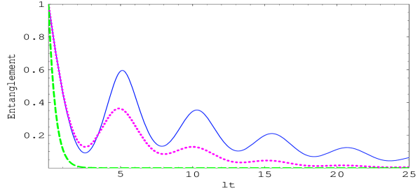
Figure 7: The same as figure 5 but E_m=200$\mu$ and different values of the decoherence parameter, where $\gamma=0.01$ (solid curve), $\gamma=0.1$ (dotted curve) and $\gamma=0.8$ (dotted-dashed curve).

This has motivated us to consider the question of how decoherence effects the scale of entanglement in the present system. The decoherence time due to the coupling to the vacuum via the probe junction can be estimated to be roughly $100$ $ns$ at the resonant condition. For the most of the experimental devices [7], this probing time restricted the upper limit of the decoherence time, since the probe junction attached to the box had a sampling time of typically $8$ $ns$. Once, the environment has been switched on, i.e., $\gamma\neq 0$, it is very clear that the decoherence plays a usual role in destroying the entanglement. In this case and for different values of the decoherence parameter $\gamma,$ we can see from figure (7) that after the onset of the interaction the entanglement function increases to reach its maximum showing strong entanglement. However its value decreases after a short period of the interaction time to reach its minimum. The function starts to increase its value again however with lower local maximum values showing a strong decay as time goes on. It is interesting to remark that decoherence due to normal decay is often said to be the most efficient effect in physics. Which means that, the entanglement increases rapidly, then approaches to a minimum value in a periodic manner. Also, from numerical results we note that with the increase of the parameter $\gamma$, a rapid decrease of the entanglement (entanglement sudden death) is shown [35].

Since the discovery of entangled sudden death [35, 25], a large number of instances of this surprising effect have been identified in the theoretical literature [44, 45, 46, 47]. In general, decay takes infinitely long, so one can wait any length of time. However, if the entanglement reaches zero in a finite time [35, 25] the game is over. Thereafter no distillation process exists that will recover any useful feature of entangled quantum joint coherence for use in quantum computing or communication [48]. These results should mark an important consideration in the design and operation of future quantum information networks. Also, properties of such entanglement decay depends on the coupling energy and qubits Josephson energies. Even if achieving the maximally entangled state is not possible in the presence of the decoherence, one can argue that finding a maximally entangled state can, under certain conditions, be achieved for a short interaction time. It is also worth noting here that we have used the simple model of a two-Cooper pair box problem, which represents a proper physical system that can be used as a qubit. This system is of a great interest because it offers the possibility of scaling to a large number of interacting qubits.

5 Conclusion

In the important context of quantum state engineering and characterization, we have studied the entanglement properties of the special class of two-coupled superconducting charge qubits. Clear physical interpretations for the maximally entangled state generation and entanglement found for certain parameter regimes of the system have been provided. In a strong coupling regime, two different types of maximally entangled states of the system have been created. This helps the comprehension of the quantitative results achieved by the use of the concurrence. Moreover, we find peculiar entanglement characteristics which are unique to this system, and which we trace back to the interplay of the various time scales of the dynamics. Our results suggest that the maximally entangled mixed state is generic in different situations for the coupled-charge qubits system, and that developing entanglement theory under other sorts of restrictions is a promising direction for further study. In a more general context, our results provide further insight into the coupled dynamics of superconducting charge qubits in the spirit of the experimental realization [3, 7, 29] and may provide a useful maximally entangled states source in the exploration of various quantum-information processing.

References

- [1] A. O. Niskanen, K. Harrabi, F. Yoshihara, Y. Nakamura, S. Lloyd, and J. S. Tsai Science, 316, 723 (2007)
- [2] For a recent review, see, e.g., J. Q. You and F. Nori, Physics Today, 58, 42 (2005); J. Q. You, J. S. Tsai, and F. Nori, Phys. Rev. B 73, 014510 (2006)
- [3] E. J. Griffith, C. D. Hill, J. F. Ralph, H. M. Wiseman and K. Jacobs, Phys. Rev. B 75, 014511 (2007)
- [4] K. B. Cooper, M. Steffen, R. McDermott, R. W. Simmonds, S.Oh, D. A. Hite, D. P. Pappas, and J. M. Martinis, Phys. Rev. Lett. 93, 180401 (2004).
- [5] Y. Nakamura, Y. A. Pashkin, and J. S. Tsai, Nature. 398, 786 (1999).
- [6] Yu. A. Pashkin, T. Yamamoto, O. Astafiev, Y. Nakamura, D. V. Averin, T. Tilma, F. Nori and J. S. Tsai, Physica C 426–431 1552 (2005).
- [7] Yu. A. Pashkin, T. Yamamoto, O. Astafiev, Y. Nakamura, D. V. Averin, J. S. Tsai, Nature 421, 823 (2003).
- [8] O. Astafiev, Yu. A. Pashkin, Y. Nakamura, T. Yamamoto, and J. S. Tsai, Phys. Rev. B 74, 094510 (2006)
- [9] M. Steffen, M. Ansmann, R. C. Bialczak, N. Katz, E. Lucero, R. McDermott, M. Neeley, E. M. Weig, A. N. Cleland, and J. M. Martinis, Science, 5792, 1423 (2006); Yu. A. Pashkin et al. Int. J. Quant. Info. 1, 421 (2003)
- [10] J. Q. You, J. S. Tsai, and F. Nori, Phys. Rev. Lett. 89, 197902 (2002).
- [11] M. A. Nielsen and I. L. Chuang, Quantum Computation and Quantum Information (Cambridge Univ. Press, 2000).
- [12] T. Yu, Phys. Lett. A 381, 287 (2007);
- [13] J. H. Eberly and Ting Yu, Science, 316, 555 (2007)
- [14] M. P. Almeida, F. de Melo, M. Hor-Meyll, A. Salles, S. P. Walborn, P. H. Souto Ribeiro, L. Davidovich, Science, 316, 579 (2007)
- [15] P. Lougovski, E. Solano, and H. Walther, Phys. Rev. A 71, 013811 (2005)
- [16] Z.-M. Zhang, A. H. Khosa, M. Ikram and M. S. Zubairy, J. Phys. B: At. Mol. Opt. Phys. 40, 1917 (2007)
- [17] X.-B. Zou and W. Mathis, Physics Letters A 337, 305 (2005)
- [18] W. P. Schleich, M. G. Raymer (Eds.), Quantum State Preparation and Measurement, J. Mod. Opt. 11–12 (1997), special issue.
- [19] W. J. Munro, D. F. V. James, A. G. White, and P. G. Kwiat, Phys. Rev. A 64, 030302 (2001); N. A. Peters, J. B. Altepeter, D. Branning, E. R. Jeffrey, T.-C. Wei, and P. G. Kwiat, Phys. Rev. Lett. 92, 133601 (2004)
- [20] T. Di and M. S. Zubairy, J. Mod. Opt. 16, 2387 (2004).
- [21] L. Diosi, in Irreversible Quantum Dynamics, edited by F. Benatti and R. Floreanini (Springer, New York, 2003), pp. 157-163.
- [22] P. J. Dodd and J. J. Halliwell, Phys. Rev. A 69, 052105 (2004); P. J. Dodd, Phys. Rev. A 69, 052106 (2004).
- [23] T. Yu and J. H. Eberly, Phys. Rev. B 66, 193306 (2002).
- [24] T. Yu and J. H. Eberly, Phys. Rev. B 68, 165322 (2003).
- [25] T. Yu and J. H. Eberly, Phys. Rev. Lett. 93, 140404 (2004)
- [26] D. Tolkunov, V. Privman and P. K. Arvind, Phys. Rev. A 71, 060308(R) (2005).
- [27] M. Abdel-Aty, J. Mod. Opt. (2007) in press, arXiv:quant-ph/0610186; M. Abdel-Aty and H. Moya-Cessa, Phys. Lett. A (2007) in press, arXiv:quant-ph/0703077.
- [28] Y. Hu, Z.-W. zhou, J.-M. Cai and G.-C. Guo, Phys. Rev. A 75, 052327 (2007)
- [29] Y. Liu, L. F. Wei, J. S. Tsai, and F. Nori, Phys. Rev. Lett. 96, 067003 (2006)
- [30] D.V. Averin, A.B. Zorin and K.K. Likharev, JETP 61, 407 (1985); D.V. Averin and C. Bruder, Phys. Rev. Lett. 91, 057003 (2003).
- [31] H.-P. Breuer and F. Petruccione, The theory of open quantum systems, Oxford University Press, Oxford, (2002)
- [32] D. A. Lidar and K. B. Whaley, in Irreversible quantum dynamics edited F.Benatti and R. Floreanini, Spring Lecutre Notes in Physics,Vol. 62, Berlin (2003), p.83.
- [33] C. W. Gardiner and P. Zoller, Quantum Noise (Springer-Verlag, Berlin, 2000).
- [34] G.J. Milburn, Phys. Rev. A 44, 5401 (1991); S. Schneider and G.J. Milburn, Phys. Rev. A 57, 3748 (1998); S. Schneider and G.J. Milburn, Phys. Rev. A 59, 3766 (1999).
- [35] T. Yu and J. H. Eberly, Phys. Rev. Lett. 97, 140403 (2006); ibid Quantum Information and Computation, (2007) in press
- [36] Y. Nakamura, Yu. A. Pashkin, and J. S. Tsai, Phys. Rev. Lett. 87, 246601 (2001).
- [37] L. Zhou, H. S. Song and C. Li, J. Opt. B: Quantum Semiclass. Opt. 4, 425 (2002)
- [38] G. Vidal and R. F. Werner, Phys. Rev. A 65, 032314 (2002); W. K. Wootters, Phys. Rev. Lett. 80 , 2245 (1998).
- [39] A. Peres, Phys. Rev. Lett. 77, 1413 (1996); M. Horodecki, P. Horodecki, and R. Horodecki, Phys. Lett. A 223, 1 (1996)
- [40] J. Lee and M. S. Kim, Phys. Rev. Lett. 84, 4236 (2000); J. Lee, M. S. Kim, Y. J. Park and S. Lee, J. Mod. Opt. 47, 2151 (2000).
- [41] S.-B. Zheng and G.-C. Guo, Phys. Rev. Lett. 85, 2392 (2000); M. Abdel-Aty, J. Opt. B: Quantum Semiclass. Opt. 5, 349 (2003).
- [42] W. K. Wootters, Phys. Rev. Lett. 80 , 2245 (1998); S.Hill and W. K. Wootters, Phys. Rev.Lett. 78, 5022 (1997).
- [43] A. Messikh, Z. Ficek and M. R. B. Wahiddin, J. Opt. B: Quantum Semiclass. Opt. 5, L1 (2003).
- [44] Z. Ficek and R. Tanaś, Phys. Rev. A 74, 024304 (2006)
- [45] L . Derkacz and L. Jakobczyk, Phys. Rev. A 74, 032313 (2006)
- [46] C. Pineda and T. H. Seligman, Phys. Rev. A 75, 012106 (2007)
- [47] K. Ann and G. Jaeger, Phys. Rev. B 75, 115307 (2007)
- [48] J. H. Eberly, private communications (2007).