Two-Component Nonlinear Schrödinger Models with a Double-Well Potential

Abstract

We introduce a model motivated by studies of Bose-Einstein condensates (BECs) trapped in double-well potentials. We assume that a mixture of two hyperfine states of the same atomic species is loaded in such a trap.The analysis is focused on symmetry-breaking bifurcations in the system, starting at the linear limit and gradually increasing the nonlinearity. Depending on values of the chemical potentials of the two species, we find numerous states, as well as symmetry-breaking bifurcations, in addition to those known in the single-component setting. These branches, which include all relevant stationary solutions of the problem, are predicted analytically by means of a two-mode approximation, and confirmed numerically. For unstable branches, outcomes of the instability development are explored in direct simulations.

I Introduction

The nonlinear Schrödinger (NLS) equation is a ubiquitous partial differential equation (PDE) with a broad spectrum of applications, including nonlinear optics in the temporal and spatial domains, matter waves, plasmas, water waves, and some biophysical models NLS ; trubatch . One of the most fundamental applications of the NLS equation stems from its direct relevance as an accurate mean-field model (known as the Gross-Pitaevskii equation, GPE, in that context) of Bose-Einstein Condensates (BECs) book1 ; book2 . The GPE usually includes an external potential accounting for the magnetic, optical or combined confinement of dilute alkali vapors that constitute the BEC reviewsbec . Basic types of such trapping potentials include parabolic and spatially periodic ones (the latter is created, as an optical lattice, by the interference of counter-propagating laser beams). The NLS equations with similar potentials are also relevant models for optical beams in graded-index waveguides and periodic waveguiding arrays kivshar ; reviewsopt .

A setting that has recently drawn much interest in the context of BECs is based on a double-well potential (DWP), which originates from a combination of the two above-mentioned types of potentials. It was realized experimentally in markus1 , leading to particularly interesting phenomena including tunneling and Josephson oscillations (for a small number of atoms), or macroscopic quantum self-trapping, with an asymmetric division of atoms between the two wells, for a large number of atoms. Numerous theoretical studies of DWP settings have been performed in parallel to the experimental work smerzi ; kiv2 ; mahmud ; bam ; Bergeman_2mode ; infeld ; todd ; theo ; carr . They addressed finite-mode reductions, analytical results for specially designed shapes of the potential, quantum effects, and other aspects of the theory (in particular, tunneling between vortex and antivortex states in BEC trapped in a two-dimensional (2D) anisotropic harmonic potential Pethik belongs to the latter category).

An interesting generalization of the DWP is provided by multi-well potentials. In particular, nonequilibrium BEC states and generation of quantum entanglement in such settings were recently studied in detail theoretically in Yuk .

Also considered were 2D 2DArik ; 2DMichal and 3D extensions of DWP settings, which add one or two extra dimensions to the model, either without any additional potential, or with an independent optical lattice acting in these directions. The extended geometry makes it possible to consider solitons, self-trapped in the extra dimension(s), which therefore emerge as effectively 1D 2DArik ; 2DMichal or 2D 3D dual-core states. The solitons may be symmetric and antisymmetric, as well as ones breaking their symmetry between the wells through bifurcations. These states may be described by simplified systems of linearly coupled 1D 2DArik or 2D 2DArik ; 3D PDEs, or, in a more accurate form, effectively 1D solitons can be found as solutions to the full two-dimensional PDE, that takes into regard a particular form of the DWP (which depends on the transverse coordinate and is uniform in the longitudinal direction, allowing the solitons to self-trap in that free direction) 2DMichal .

DWPs are also relevant to nonlinear-optics settings, such as the twin-core self-guided laser beams in Kerr media HaeltermannPRL02 , optically induced dual-core waveguiding structures in a photorefractive crystal zhigang , and DWP configurations for trapped light beams in a structured annular core of an optical fiber Longhi . As concerns DWPs with extra dimensions, their counterparts in fiber optics are twin–core fibers dual-core-fiber and fiber Bragg gratings dual-core-FBG that were shown to support symmetric and asymmetric solitons. In addition, also investigated was the symmetry breaking of solitons in models of twin-core optical waveguides with non-Kerr nonlinear terms, viz, quadratic dual-core-quadratic and cubic-quintic (CQ) dual-core-CQ . All these optical model are based on systems of linearly coupled 1D PDEs. Also in the context of nonlinear optics, a relevant model is based on a system of linearly coupled complex Ginzburg-Landau equations with the CQ nonlinearity, that gives rise to stable dissipative solitons with broken symmetry Ariel .

In addition to the linearly coupled systems of two nonlinear PDEs motivated by the DWP transverse structures, several models of triangular configurations, which admit their own specific modes of the symmetry breaking, have also been introduced in optics, each model based on a system of three nonlinear PDEs with symmetric linear couplings between them. These include tri-core nonlinear fibers Buryak and fiber Bragg gratings Arik , as well as a system of three coupled Ginzburg-Landau equations with the intra-core nonlinearity of the CQ type Skryabin .

The significant interest in the DWP settings has also motivated the appearance of rigorous mathematical results regarding the symmetry-breaking bifurcations and the stability of nonlinear stationary states kirr . A rigorous treatment was also developed for the dynamical evolution in such settings bambusi1 ; bambusi2 .

Our objective in this work is to extend the realm of DWPs to multi-component settings. This is of particular relevance to experimental realizations of BEC – e.g.,, in a mixture of different hyperfine states of ⁸⁷Rb book1 ; book2 (see also very recent experiments reported in Ref. hall and references therein). This extension is relevant to optics too, where multi-component dynamics can be, for instance, realized in photorefractive crystals zhigang2 . In the one-component setting, the analysis of the weakly nonlinear regime has given considerable insight into the emergence of asymmetric branches from symmetric or anti-symmetric ones, in the models with self-focusing and self-defocusing nonlinearity, respectively), and the destabilization of the “parent” branches through the respective symmetry-breaking bifurcations, as well as the dynamics initiated by the destabilization smerzi ; kiv2 ; Bergeman_2mode ; todd ; theo ; kirr .

In the present work, we aim to extend the analysis of the DWP setting to two-component systems. In addition to the finite-mode approximation, which can be justified rigorously kirr under conditions that remain valid in the present case, we use numerical methods to follow the parametric evolution of solution branches that emerge from bifurcations in the two-component system. We observe that, in addition to the branches inherited from the single-component model, new branches appear with the growth of the nonlinearity. We dub these new solutions “combined” ones, as they involve both components. In fact, the new branches connect some of the single-component ones. Furthermore, these new branches may undergo their own symmetry-breaking bifurcations. The solutions depend on chemical potentials of the two species, $\mu_{1}$ and $\mu_{2}$ (in terms of BEC), and, accordingly, loci of various bifurcations will be identified in plane $\left(\mu_{1},\mu_{2}\right)$.

The paper is structured as follows. In Section II, we present the framework of the two-component problem, including the two-mode reduction (in each component), that allows us to considerably simplify the existence and stability problems. The formulation includes also a physically possible linear coupling between the components, but the actual analysis is performed without the linear coupling. In section III, we report numerical results concerning the existence and stability of the new states, as well as the evolution of unstable ones. In section IV, we summarize the findings and discuss directions for further studies.

II Analytical consideration

As a prototypical model that is relevant both to BECs book1 ; book2 and optics kivshar , we take the normalized two-component NLS equation of the following form:

$$\begin{split}iu_{t}&=Lu+\kappa v+\sigma(|u|^{2}+g|v|^{2})u-\mu_{1}u,\\ iv_{t}&=Lv+\kappa u+\sigma(|v|^{2}+g|u|^{2})v-\mu_{2}v,\end{split}$$ (1)

where $u$ and $v$ are the wave functions of the two BEC components, or local amplitudes of the two optical modes, $\mu_{1,2}$ are chemical potentials in BEC or propagation constants in the optical setting, $\kappa$ is the coefficient of the linear coupling between the components, and

$$L=-(1/2)\partial_{x}^{2}+V(x)$$ (2)

is the usual single-particle operator with trapping potential $V(x)$. The repulsive or attractive character of the nonlinearity in BEC (self-defocusing or self-focusing, in terms of optics) is defined by $\sigma=+1$ and $\sigma=-1$, respectively, while $\sigma g$ is the coefficient of the inter-species interactions in BEC, or cross-phase modulation (XPM) in optics.

In the case of (for instance) two hyperfine states with $|F,m_{F}>=|1,-1>$ and $|2,1>$ in ⁸⁷Rb, both coefficients of the self-interaction and the cross-interaction coefficient are very close, although their slight difference is critical in accounting for the immiscibility of the two species (see, e.g.,, hall and references therein). However, for problems considered below, the difference does not play a significant role, hence we set $g=1$ in Eqs. (1), which corresponds to the Manakov’s system, i.e., one which is integrable, in the absence of the potential, $V(x)=0$ in Eq. (2) manakov ; kivshar . In fact, $V(x)$ is the DWP, which we compose of a parabolic trap (with corresponding frequency $\Omega$) and a $\mathrm{sech}^{2}$-shaped barrier (of strength $V_{0}$ and width $w$) in the middle:

$$V(x)=(1/2)\Omega^{2}x^{2}+V_{0}\mathrm{sech}^{2}\left(x/W\right).$$ (3)

The calculations presented below have been performed for $\Omega=0.1$, $V_{0}=1$ and $W=0.5$, in which case the first two eigenvalues of linear operator (2) are $\omega_{0}=0.1328$ and $\omega_{1}=0.1557$. However, we have checked that the generic picture presented below is insensitive to specific details of the potential, provided that it is symmetric.

The linear coupling in Eqs. (1), via the terms proportional to $\kappa$, accounts for the possibility of interconversion between the two hyperfine states in the BEC mixture, which may be induced, e.g.,, by appropriate two-photon pulses in the situation considered in Ref. hall . In optics, the linear coupling is induced by a twist of the optical waveguide, if the two wave components correspond to orthogonal linear polarizations of light.

To define an appropriate basis for the finite-mode expansion of solutions to Eqs. (1), we first consider the following eigenvalue problem,

$$\begin{pmatrix}L&\kappa\\ \kappa&L\end{pmatrix}\begin{pmatrix}u\\ v\end{pmatrix}=\omega\begin{pmatrix}u\\ v\end{pmatrix}.$$ (4)

We denote the ground and first excited eigenstates of the matrix operator in Eq. (4), which appertain to the two lowest eigenvalues, as $\left\{u_{0},v_{0}\right\}$ and $\left\{u_{1,}v_{1}\right\}$ (these two states are, as usual, spatially even and odd ones, respectively). The Hermitian nature of the linear operator in Eq. (4) ensures that the eigenvalues are real, and the eigenfunctions can also be chosen in a real form. In fact, in the case that we will examine here, we will have $u_{0}=v_{0}$ and $u_{1}=v_{1}$, but the different notations will be kept for the $u$ and $v$ components, to demonstrate how the nonlinear analysis can be carried out in the general case. Then, the two-mode approach is based on the assumption that, in the weakly nonlinear case, the solution is decomposed as a linear combination of these eigenfunctions, i.e.,

$$\begin{split}u(x,t)&=c_{0}(t)u_{0}(x)+c_{1}(t)u_{1}(x),\\ v(x,t)&=c_{2}(t)v_{0}(x)+c_{3}(t)v_{1}(x).\end{split}$$ (5)

This assumption can be rigorously substantiated, with an estimate for the accuracy, upon imposing suitable conditions on the smallness of the nonlinearity, and properties of the rest of the linear spectrum kirr . Therefore, as shown in kirr , such an approach can be controllably accurate for small $N=\int_{-\infty}^{+\infty}\left(|u|^{2}+|v|^{2}\right)dx$, although below we examine its comparison with numerical results even for values of $N$ of O$(1)$.

It is relevant to mention that an alternative approach to the decomposition of the two-component wave functions could be based on using the basis of symmetric and antisymmetric wave functions, $u_{0}\pm v_{0}$ and $u_{1}\pm v_{1}$. However, the resort to this basis does not make the final equations really simpler. On the other hand, unlike the approach developed below, the use of the alternative basis would make it much harder to estimate the error of the finite-mode approximation, and thus rigorously substantiate the approximation, cf. Ref. kirr .

Substituting ansatz (5) in Eqs. (1), and projecting the resulting equations onto eigenfunctions $\left\{u_{0},v_{0}\right\}$ and $\left\{u_{1,}v_{1}\right\}$, one can derive at the following nonlinear ODEs for the temporal evolution of the complex amplitudes of the decomposition, $c_{0,1,2,3}$:

$$\begin{split}i\dot{c_{0}}=(\omega_{0}-\mu_{1})c_{0}+\kappa c_{2}&+\sigma[\Gamma_{0000}|c_{0}|^{2}c_{0}+\Gamma_{0011}(c_{1}^{2}c_{0}^{\ast}+2c_{0}|c_{1}|^{2})]\\ &+\sigma g[\Gamma_{0000}c_{0}|c_{2}|^{2}+\Gamma_{0011}(c_{0}|c_{3}|^{2}+c_{1}c_{2}c_{3}^{\ast}+c_{1}c_{2}^{\ast}c_{3})],\end{split}$$ (6)

$$\begin{split}i\dot{c_{1}}=(\omega_{1}-\mu_{1})c_{1}+\kappa c_{3}&+\sigma[\Gamma_{1111}|c_{1}|^{2}c_{1}+\Gamma_{0011}(c_{0}^{2}c_{1}^{\ast}+2|c_{0}|^{2}c_{1})]\\ &+\sigma g[\Gamma_{1111}c_{1}|c_{3}|^{2}+\Gamma_{0011}(c_{1}|c_{2}|^{2}+c_{0}c_{2}c_{3}^{\ast}+c_{0}c_{2}^{\ast}c_{3})],\end{split}$$ (7)

$$\begin{split}i\dot{c_{2}}=(\omega_{0}-\mu_{2})c_{2}+\kappa c_{0}&+\sigma[\Gamma_{0000}|c_{2}|^{2}c_{2}+\Gamma_{0011}(c_{3}^{2}c_{2}^{\ast}+2c_{2}|c_{3}|^{2})]\\ &+\sigma g[\Gamma_{0000}|c_{0}|^{2}c_{2}+\Gamma_{0011}(|c_{1}|^{2}c_{2}+c_{0}c_{1}^{\ast}c_{3}+c_{0}^{\ast}c_{1}c_{3})],\end{split}$$ (8)

$$\begin{split}i\dot{c_{3}}=(\omega_{1}-\mu_{2})c_{3}+\kappa c_{1}&+\sigma[\Gamma_{1111}|c_{3}|^{2}c_{3}+\Gamma_{0011}(c_{2}^{2}c_{3}^{\ast}+2|c_{2}|^{2}c_{3})]\\ &+\sigma g[\Gamma_{1111}|c_{1}|^{2}c_{3}+\Gamma_{0011}(|c_{0}|^{2}c_{3}+c_{0}c_{1}^{\ast}c_{2}+c_{0}^{\ast}c_{1}c_{2})].\end{split}$$ (9)

In these equations, $\Gamma_{ijkl}\equiv\int_{-\infty}^{+\infty}u_{i}(x)u_{j}(x)u_{k}(x)u_{l}(x)dx$ are the so-called matrix elements of the nonlinear four-wave interactions, with $\Gamma_{ijkl}=0$ when $i$+$j$+$k$+$l$ is odd.

Seeking for real fixed points to Eqs. (6) - (9), $a_{j}(t)\equiv\rho_{j}$, we reduce the equations to an algebraic system,

$$\begin{split}\mu_{1}\rho_{0}=(\omega_{0}\rho_{0}+\kappa\rho_{2})&+\sigma(\Gamma_{0000}\rho_{0}^{3}+3\Gamma_{0011}\rho_{0}\rho_{1}^{2})\\ &+\sigma g(\Gamma_{0000}\rho_{0}\rho_{2}^{2}+\Gamma_{0011}\rho_{0}\rho_{3}^{2}+2\Gamma_{0011}\rho_{1}\rho_{2}\rho_{3}),\end{split}$$ (10)

$$\begin{split}\mu_{1}\rho_{1}=(\omega_{1}\rho_{1}+\kappa\rho_{3})&+\sigma(\Gamma_{1111}\rho_{1}^{3}+3\Gamma_{0011}\rho_{0}^{2}\rho_{1})\\ &+\sigma g(\Gamma_{1111}\rho_{1}\rho_{3}^{2}+\Gamma_{0011}\rho_{1}\rho_{2}^{2}+2\Gamma_{0011}\rho_{0}\rho_{2}\rho_{3}),\end{split}$$ (11)

$$\begin{split}\mu_{2}\rho_{2}=(\omega_{0}\rho_{2}+\kappa\rho_{0})&+\sigma(\Gamma_{0000}\rho_{2}^{3}+3\Gamma_{0011}\rho_{2}\rho_{3}^{2})\\ &+\sigma g(\Gamma_{0000}\rho_{0}^{2}\rho_{2}+\Gamma_{0011}\rho_{1}^{2}\rho_{2}+2\Gamma_{0011}\rho_{0}\rho_{1}\rho_{3}),\end{split}$$ (12)

$$\begin{split}\mu_{2}\rho_{3}=(\omega_{1}\rho_{3}+\kappa\rho_{1})&+\sigma(\Gamma_{1111}\rho_{3}^{3}+3\Gamma_{0011}\rho_{2}^{2}\rho_{3})\\ &+\sigma g(\Gamma_{1111}\rho_{1}^{2}\rho_{3}+\Gamma_{0011}\rho_{0}^{2}\rho_{3}+2\Gamma_{0011}\rho_{0}\rho_{1}\rho_{2}),\end{split}$$ (13)

The simplest solution to the above equations can be obtained in the form of $\rho_{2}=\rho_{0}$ and $\rho_{3}=\rho_{1}$, for $\mu_{1}=\mu_{2}$. With this substitution, the remaining equations are

$$\begin{split}\mu_{1}-\tilde{\omega}_{0}&=\tilde{\sigma}(\Gamma_{0000}\rho_{0}^{2}+3\Gamma_{0011}\rho_{1}^{2}),\\ \mu_{1}-\tilde{\omega}_{1}&=\tilde{\sigma}(\Gamma_{1111}\rho_{1}^{2}+3\Gamma_{0011}\rho_{0}^{2}),\end{split}$$ (14)

where $\tilde{\omega}_{0}\equiv\omega_{0}+\kappa,\;\tilde{\omega}_{1}\equiv\omega_{1}+\kappa,\;\tilde{\sigma}\equiv\sigma(1+g).$ System (14) can be solved as a linear one for $\rho_{0,1}^{2}$. For given values of $\Gamma$ and $\omega$, a physical range of chemical potential $\mu_{1}$ is that which provides physical solutions for $\rho_{0,1}^{2}$.

In what follows, we focus on the case of $\kappa=0$, since $\kappa\neq 0$ imposes the condition $\mu_{1}=\mu_{2}$, while we are interested in more general solutions. With $\kappa=0$, chemical potentials $\mu_{1}$ and $\mu_{2}$ may be different, allowing us to explore the two-parameter solution space $(\mu_{1},\mu_{2})$, for both signs of the nonlinearity, self-attractive ($\sigma=-1$) and the self-repulsive ($\sigma=+1$).

The simplest possible branches of solutions are single-mode ones, with only one of amplitudes $\rho_{j}$ different from zero. Branches of these solutions can be easily found from Eqs. (10) - (13),

$$\begin{split}\rho_{0}^{2}&=\frac{\mu_{1}-\omega_{0}}{\sigma\Gamma_{0000}}\neq 0,\quad\rho_{1}=\rho_{2}=\rho_{3}=0\\ \rho_{1}^{2}&=\frac{\mu_{1}-\omega_{1}}{\sigma\Gamma_{1111}}\neq 0,\quad\rho_{0}=\rho_{2}=\rho_{3}=0\\ \rho_{2}^{2}&=\frac{\mu_{2}-\omega_{0}}{\sigma\Gamma_{0000}}\neq 0,\quad\rho_{0}=\rho_{1}=\rho_{3}=0\\ \rho_{3}^{2}&=\frac{\mu_{2}-\omega_{1}}{\sigma\Gamma_{1111}}\neq 0,\quad\rho_{0}=\rho_{1}=\rho_{2}=0\end{split}$$ (15)

The first one of these branches contains the projection only onto the even (symmetric0 eigenfunction of the first component, and will hereafter be accordingly denoted S1. Similarly, the second branch has a projection onto the odd (antisymmetric) mode of the first component, and will be named AN1. The third and fourth solutions are similar modes in the second component, to be denoted S2 and AN2, respectively.

In addition to these modes, there exist asymmetric states in each of the components (similar to the one-component model theo ; kirr ),

$$\rho_{0}^{2} = \frac{\Gamma_{1111}(\mu_{1}-\omega_{0})-3\Gamma_{0011}(\mu_{1}-\omega_{1})}{\sigma(\Gamma_{1111}\Gamma_{0000}-9\Gamma_{0011}^{2})},\quad\rho_{2}=0,$$ (16)

$$\rho_{1}^{2} = \frac{\Gamma_{0000}(\mu_{1}-\omega_{1})-3\Gamma_{0011}(\mu_{1}-\omega_{0})}{\sigma(\Gamma_{1111}\Gamma_{0000}-9\Gamma_{0011}^{2})},\quad\rho_{3}=0.$$ (17)

Since these solutions do not exist in the linear limit, they have to bifurcate at a non-zero value of the amplitude, from either symmetric or antisymmetric branches (15). In fact, such solutions bifurcate, depending on the sign of $\sigma$ and coefficients $\Gamma$, either from S1 at

$$\mu_{1}^{\mathrm{(cr)}}={\omega_{1}}-\frac{3\Gamma_{0011}({\omega_{0}}-{\omega_{1}})}{\Gamma_{0000}-3\Gamma_{0011}},$$ (18)

or from AN1 at

$$\mu_{1}^{\mathrm{(cr)}}={\omega_{0}}-\frac{3\Gamma_{0011}({\omega_{1}}-{\omega_{0}})}{\Gamma_{1111}-3\Gamma_{0011}}.$$ (19)

The asymmetric solutions given by Eqs. (16) and (17) will be denoted AS1. Similarly, there is an asymmetric branch of solutions in the second component, hereafter denoted AS2, with

$$\rho_{2}^{2} = \frac{\Gamma_{1111}(\mu_{2}-\omega_{0})-3\Gamma_{0011}(\mu_{2}-\omega_{1})}{\sigma(\Gamma_{1111}\Gamma_{0000}-9\Gamma_{0011}^{2})},\quad\rho_{0}=0$$ (20)

$$\rho_{3}^{2} = \frac{\Gamma_{0000}(\mu_{2}-\omega_{1})-3\Gamma_{0011}(\mu_{2}-\omega_{0})}{\sigma(\Gamma_{1111}\Gamma_{0000}-9\Gamma_{0011}^{2})},\quad\rho_{1}=0,$$ (21)

and conclusions that can be deduced about its bifurcation are similar to those concerning AS1.

In addition to these obvious solutions, there exist others, that can be obtained as solutions to Eqs. (10)-(13) and involve both components (obviously, they have no counterparts in the single-component model). They will be denoted as “combined” ones (C1, C2, C3 and C4) in what follows. Although they cannot be expressed by simple analytical formulas, unlike the S, AN and AS branches that were defined above, they can be easily found as numerical solutions of Eqs. (10)-(13), and will be compared to full numerical results in the following section.

III Numerical Results

We start the numerical analysis by examining the self-focusing case. Because of the complexity of the bifurcation diagrams in the plane of the chemical potentials of the two components, $\left(\mu_{1},\mu_{2}\right)$, we will illustrate the bifurcation phenomenology by showing cross-sections of the full two-parameter bifurcation diagram for varying $\mu_{1}$, at different fixed values of $\mu_{2}$.

In connection to the single-component states presented above, four distinct scenarios have been found, when the second chemical potential, $\mu_{2}$, appears. The first (most complex) scenario takes place at $\mu_{2}<\mu_{2}^{\mathrm{(cr)}}$ (with some critical value $\mu_{2}^{\mathrm{(cr)}}$), when branch AS2 exists (in addition to S2 and AN2). The second case is observed in region $\mu_{2}^{\mathrm{(cr)}}<\mu_{2}<\omega_{0}$, in which case only S2 and AN2 exist (recall $\omega_{0}$ and $\omega_{1}$ are two lowest eigenvalues of operator (2)). The third scenario is found in the interval of $\omega_{0}<\mu_{2}<\omega_{1}$, where only branch AN2 may exist, and, finally, the fourth one takes place at $\omega_{1}<\mu_{2},$ where there are no single-component solutions for the second field (in the case of the self-attractive nonlinearity).

We describe the most complex of these scenarios in Fig. 1 and subsequently summarize differences from this case in the remaining three simpler regimes. In Fig. 1, the top panel presents the full numerically generated bifurcation diagram, in terms of total norm $N=\int_{-\infty}^{+\infty}\left(|u|^{2}+|v|^{2}\right)dx$ (which is proportional to the total number of atoms in both species in the BEC model, or the total beam power in optics) as a function of $\mu_{1}$ for fixed $\mu_{2}=0.1$. The horizontal lines in this diagram represent single-component solutions AS2, S2 and AN2 in the second field (in order of the increasing norm), which are, obviously, unaffected by the variation of $\mu_{1}$ of the other component, that remains “empty” in these solutions. As the asymmetric branch AS2 exists at this value of $\mu_{2}$ (in fact, at all values in region $\mu_{2}<\mu_{2}^{\mathrm{(cr)}}$), it is stable (as the one generated by the symmetry-breaking bifurcation in the single-component equation theo ; kirr ), while branch S2 is destabilized by the same bifurcation. In addition to these branches represented solely by the second component, with the variation of $\mu_{1}$ we observe the emergence of the single-component branches, S1 and AN1, in the first field, from the corresponding linear limit, at $\mu_{1}=\omega_{0}$ and $\mu_{1}=\omega_{1}$. In addition, past critical point $\mu_{1}^{\mathrm{(cr)}}=0.1214$, the symmetry-breaking-induced branch AS1 arises in the first component, destabilizing its symmetric “parent branch” S1, in agreement with the known results for the one-component model.

An additional explanation is necessary about the special case of $\mu_{1}=\mu_{2}$ ($=0.1$ in the case of Fig. 1). In that case, we observe that branches S1 and S2, as well as AN1 and AN2, and also AS1 and AS2, collide. At this value of the parameter, stationary equations (1) (with $u_{t}=v_{t}=0$) are degenerate (recall we consider the case of $g=0$), making any solution in the form of $au=bv$ is possible, including pairs $(a,b)=(0,1)$ (which corresponds to the branches considered above that contain only the first component), $(a,b)=(1,0)$ (i.e., the second-component branches), and $(a,b)=(1,1)$ (where the two components are identical). Therefore, in this degenerate case, the points of collisions of the branches in the bifurcation diagram of Fig. 1 actually denote a one-parameter family of solutions, rather than an isolated solution.

The key new feature of this bifurcation diagram in comparison to its one-component counterpart is the presence of the four new branches of solutions, C1 through C4. Two of them are found to connect (“bridge”) two single-component branches of the solutions belonging to different components, and two other species of the new solutions bifurcate from the bridging ones. More specifically, as can be seen in the bottom left panel of Fig. 1 (which is a blowup of the one in the top left corner), branch C2 interpolates between antisymmetric branch AN2 of the second component and symmetric branch S1 of the first component (hence, one may naturally expect that the solutions belonging to C2 have symmetric and antisymmetric profiles in the first and second components, respectively, see Figs. 5-7 below. Furthermore, similarly to the bifurcation of the asymmetric branches from the symmetric ones in the single-component models, there is such a bifurcation which occurs to the C2 branch, destabilizing it and giving rise to a stable branch C1 of combined solutions, with asymmetric profiles instead of the symmetric and antisymmetric waveforms in the first and second components of C2, respectively (see Fig. 6 below).

Naturally, there is a similar pair of two-component branches emerging due to the bridging of S2 and AN1. As expected, the two-component branch C4, which is responsible for the bridging per se, features symmetric and antisymmetric profiles in its second and first components. Finally, it is clearly seen in the bottom right panel of Fig. 1 (which is a blowup of another relevant fragment of the top left panel) that a symmetry-breaking bifurcation occurs on branch C4, which destabilizes it and gives rise to branch C3 of stable asymmetric two-component solutions. It is worthy to note that this emerging asymmetric branch C3 terminates through a collision with the single-component asymmetric branch AS2, as can also be seen in the top left panel of Fig. 1.

Similar to the emergence of AS1 from S1, the bifurcation of C1 from C2 and of C3 from C4 are of the pitchfork type. Therefore, we actually have two asymmetric branches of types C1 and C3, which are mirror images to each other (accordingly, the additional asymmetric waveforms can be obtained from those displayed in Fig. 7 by the reflection around $x=0$).

Comparing this complex bifurcation picture with predictions of algebraic equations (10)-(13), we conclude that the picture is captured in its entirety by the two-mode approximation, as shown in the top right panel of Fig. 1. Although some details may differ (notice, in particular, slight disparity in the scales of the two diagrams in the top panels of Fig. 1), the overall structure of the diagrams is fully reproduced by the algebraic equations. As a characteristic indicating the accuracy of the approximation, it is relevant to compare the bifurcation points. In the finite-mode picture, the bifurcation of AS1 from S1 occurs at $\mu_{1}=0.1211$, C1 bifurcates from C2 at $\mu_{1}=0.0780$, and the bifurcation of C3 from C4 happens at $\mu_{1}=0.1225$. The full numerical results yield the following values for the same bifurcation points: $\mu_{1}=0.1214$, $\mu_{1}=0.0781$ and $\mu_{1}=0.1224$, respectively, with the relative error $<0.25\%$.

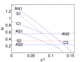
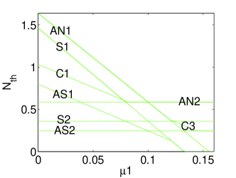
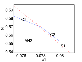
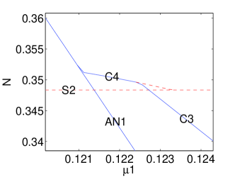
Figure 1: (Color online) Top panel: The norm (corresponding to the number of atoms in BEC and total power in optics) of the numerically found solutions of Eq. (1) (left) and their counterparts predicted by the two-mode approximation (right) for the self-attractive nonlinearity ($\sigma=-1$), as a function of $\mu_{1}$, for $\mu_{2}=0.1$. Here and in other figures, the (blue) solid lines and (red) dashed ones depict stable and unstable solutions, respectively. The bottom panels are blowups of segments in the top left panel where bifurcations involving the new combined solutions occur. S1, AN1, AS1 and S2, AN2, AS2 mark, respectively, symmetric, antisymmetric, and asymmetric single-component solutions belonging to fields $u$ or $v$. Symbols C1, C2, C3, C4 mark branches of the new combined (two-component) solutions, which are defined in the text.

Two additional descriptions of these bifurcations, which help to understand the emergence of the combined branches, are presented in Figs. 2 and 3. The former one shows norms $N_{u}=\int_{-\infty}^{+\infty}|u|^{2}dx$ and $N_{v}=\int_{-\infty}^{+\infty}|v|^{2}dx$, and the latter figure shows the total number of atoms in the left and right wells, $N_{L}=\int_{-\infty}^{0}\left(|u|^{2}+|v|^{2}\right)dx$ and $N_{R}=\int_{0}^{\infty}\left(|u|^{2}+|v|^{2}\right)dx$, as functions of the chemical potential $\mu_{1}$. The left panels are produced by the numerical solution of the stationary version of underlying GPEs, Eqs. (1), while the right panels correspond to the finite-mode approximation. Notice a sharp (near vertical) form of the combined branches C2 and C4 in the former figure, which indicates a short interval of their existence, and their change of stability upon the collision with (or, more appropriately, the bifurcation of) C1 and C3, respectively. In the latter figure, it is worthwhile to notice the similarity of the curves for $N_{L}$ and $N_{R}$ appertaining to branches S1, AN1, S2 and AN2, in contrast with the differences between the respective curves for AS1, AS2 and combined branches C1 and C3, which indicates the asymmetry between the states trapped in the two wells in the latter case.

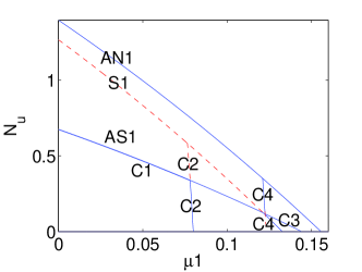
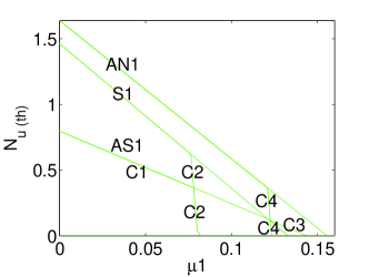
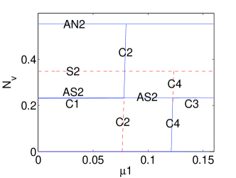
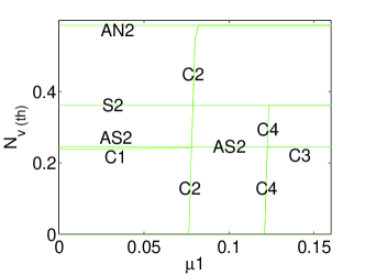
Figure 2: (Color online) The norm of the numerically found (left) and approximate two-mode (right) wave functions $u$ (top) and $v$ (bottom) of solutions to the stationary version of Eq. (1) with the attractive nonlinearity ($\sigma=-1$), as a function of $\mu_{1}$, for $\mu_{2}=0.10$. The notation is the same as in Fig. 1.

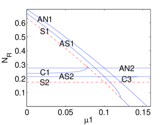
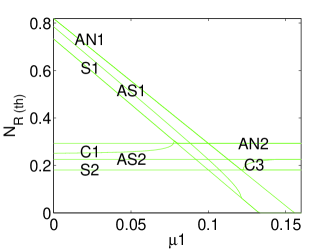
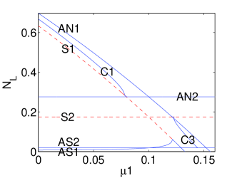
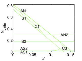
Figure 3: (Color online) The norms of the right (top) and left (bottom) parts of the wave functions, $N_{R}=\int_{0}^{+\infty}|u|^{2}+|v|^{2}dx$, and $N_{L}=\int_{-\infty}^{0}|u|^{2}+|v|^{2}dx$, as obtained from the numerical (left) and approximate two-mode (right) solutions of Eq. (1) with the attractive nonlinearity ($\sigma=-1$), as a function of $\mu_{1}$, for $\mu_{2}=0.10$. The notation is the same as in Fig. 1. Notice that, as in the top left panel of Fig. 1, the branches C2 and C4 are actually indiscernible.

Having addressed the most complex bifurcation scenario observed at $\mu_{2}<\mu_{2}^{\mathrm{(cr)}}$, we now turn to the three remaining cases, namely, $\mu_{2}^{\mathrm{(cr)}}<\mu_{2}<\omega_{0}$, $\omega_{0}<\mu_{2}<\omega_{1}$, and $\omega_{1}<\mu_{2}$. Full numerically generated bifurcation diagrams for each of these cases can be found in the left panels of Fig. 4, while the corresponding results produced by algebraic equations (10)-(13) are presented in the right panels. Once again, we notice a very good agreement between the two sets of the results. In interval $\mu_{2}^{\mathrm{(cr)}}<\mu_{2}<\omega_{0}$, the main difference from the case shown in Fig. 1 is that, as concerns the single-component branches belonging to the second field, the asymmetric branch AS2 has not bifurcated from the symmetric one S2, therefore S2 is a stable branch. As a result, the two-component branches C4 and C3 do not exist in this case (in particular, the existence of C3 is not possible topologically, since it would destabilize C4 which would subsequently have to merge with stable branch S2).

Nevertheless, the behavior of branches C1 and C2 remains the same as before. In the middle panels of Fig. 4, which represents the case of $\omega_{0}<\mu_{2}<\omega_{1}$, the situation is simpler in that branch S2 does not exist (in this regime, only branch AN2 exists in the second component), hence the presence of C3 and C4, that would connect S2 to AN1, is impossible. Finally, in the case of $\omega_{1}<\mu_{2}$, there are no single-component branches in the second field; as a result, even the two-component branch C2, joining AN2 and S1, has to disappear (hence C1 bifurcating from it cannot exist either), and we are therefore left solely with the single-component solutions for $u$ (only the branches S1, AN1 and AS1 are present).

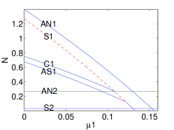
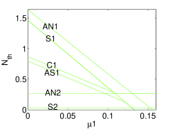
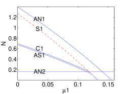
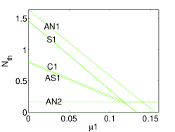
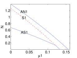
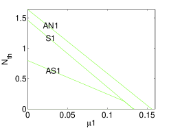
Figure 4: (Color online) The norm of the numerical (left) and approximate two-mode (right) stationary solutions of Eq. (1) for the attractive nonlinearity ($\sigma=-1$) as a function of $\mu_{1}$ for $\mu_{2}=0.13$ (top), $\mu_{2}=0.14$ (middle), and $\mu_{2}=0.16$ (bottom). The notation is the same as in Fig. 1.

Examples of solutions representing all the branches considered above are shown in Figs. 5-7. Figure 5 represents the three branches that have only the $u$ component, namely S1, AN1 and AS1 in the left, middle and right panels of the figure, for $\mu_{1}=0.04$ and $\mu_{2}=0.1$. Notice that, since solution AS1 exists for this parameter sets, solution S1 is unstable, while AN1 and AS1 are stable.

The results of the linear-stability analysis around the solutions are shown in the bottom panels of the figure. For the purpose of this analysis, perturbed versions of stationary solutions $\left\{u_{0}(x),v_{0}(x)\right\}$ are taken as

$$u(x,t) = u_{0}(x)+\epsilon\left(U_{1}(x)e^{\lambda t}+U_{2}^{\star}(x)e^{\lambda^{\star}t}\right),$$ (22)

$$v(x,t) = v_{0}(x)+\epsilon\left(V_{1}(x)e^{\lambda t}+V_{2}^{\star}(x)e^{\lambda^{\star}t}\right),$$ (23)

where $\epsilon$ is an infinitesimal amplitude of perturbations, and the resulting linearized equations for eigenvalue $\lambda$ and eigenvector $(U_{1},U_{2},V_{1},V_{2})^{T}$ are solved numerically. As usual, instability is manifested by the existence of eigenvalue(s) $\lambda$ with a non-zero real part. The stability results are shown in terms of the spectral plane $(\lambda_{r},\lambda_{i})$ for $\lambda=\lambda_{r}+i\lambda_{i}$, hence the instability corresponds to the presence of an eigenvalue in the right-hand half-plane (for example, for branch S1 in Fig. 5). Very similar results to those displayed in Fig. 5 can be obtained for solutions S2, AN2 and AS2, in which only the second component is nonzero (because they are direct counterparts to those in Fig. 5, they are not shown here).

The combined solutions emerging due to the bridging of the single-component branches are shown in Figs. 6 and 7. The former figure shows two instances of branch C2 (right and middle panels), before and after the bifurcation of branch C1 (the latter one is shown in the left panel). The stability features of these solutions are displayed in the bottom panels of the figure. Similar features are shown in Fig. 7 for two-components branches C4 and C3.

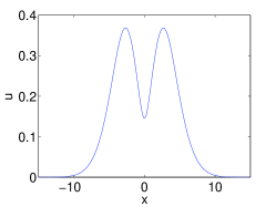
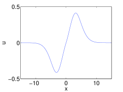
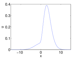
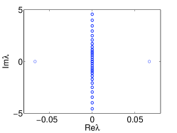
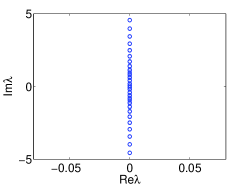
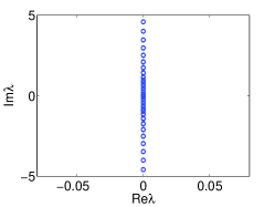
Figure 5: (Color online) Top panel: profiles of wave function $u$ corresponding to the symmetric (left), antisymmetric (middle) and asymmetric (right) branches of the single-component solutions, S1, AN1, and AS1, respectively, in Fig. 1 for $\mu_{1}=0.04$. Bottom panel: the result of the linear-stability analysis around S1 (left), AN1 (middle) and AS1 (right), in the complex plane of (Re$\lambda$, Im$\lambda$). The existence of an eigenvalue with a positive real part implies instability of the solution.

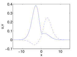
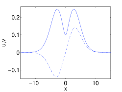
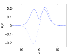
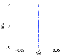
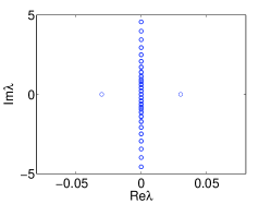
Figure 6: (Color online) Profiles of wave functions $u$ (top), $v$ (middle) and respective stability eigenvalues (bottom) which correspond to two-component solutions C1 and C2 (branches of these solutions are shown in Fig. 1): C1 for $\mu_{1}=0.04$ (left), C2 for $\mu_{1}=0.0774$ (middle), and C2 for $\mu_{1}=0.0786$ (right).

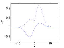
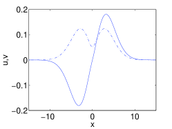
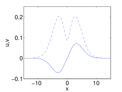
Figure 7: Profiles of wave functions $u$ and $v$ (top panel’s solid and dash-dotted line, respectively) and stability eigenvalues (bottom) corresponding to two-component solutions C3 and C4 (the branches of these solutions are shown in Fig. 1): C3 for $\mu_{1}=0.135$ (left), C4 for $\mu_{1}=0.122$ (middle), and C4 for $\mu_{1}=0.123$ (right).

We now turn to the self-defocusing case (corresponding to repulsive interatomic interactions in BEC), with $\sigma=1$ in Eqs. (1). The results are shown in Figs. 8-9. In this case, we do not show profiles of solutions belonging to various branches, as they are very similar to those obtained in the model with the self-attraction, the only difference being that their spatial size is larger, due to the self-repulsive nature of the nonlinearity.

We again distinguish the main regimes, namely, $\mu_{2}^{\mathrm{(cr)}}<\mu_{2}$, when all three branches S2, AN2 and AS2 exist; $\omega_{1}<\mu_{2}<\mu_{2}^{\mathrm{(cr)}}$, for which only S2 and AN2 exist; $\omega_{0}<\mu_{2}<\omega_{1}$, when only S2 is present; and $\mu_{2}<\omega_{0}$, for which there is no branch of single-component solutions in the $v$ field. The first (and most complex) of these regimes is shown in Fig. 8, in direct analogy to Fig. 1 for the focusing case. Once again, we observe the presence (in addition to the three single-component branches in the $u$ field, and three such branches in the $v$ field) of four families of the combined solutions. In Fig. 8, C2 (with symmetric $u$ and anti-symmetric $v$ components) bridges stable branch S2 and unstable one AN1, while branch C1 of stable two-component asymmetric solutions bifurcates from C2, making it unstable. There is also branch C4 which links S1 and AN2, and C3, which bifurcates from C4 and terminates by merging into AS2. Details of this picture are shown in the bottom panels of Fig 8. To highlight the accuracy of the approximation based on algebraic equations (10)-(13), we display the bifurcation diagram predicted by this approximation in the top right panel of Fig. 8, which confirms that all the bifurcations and branches are captured within the two-mode framework. As a measure of the agreement between the approximate and numerical results, we again present coordinates of the bifurcation points: AS1 emerges from AN1 at $\mu_{1}=0.1684$ according to the numerical results, while the approximation predicts this to happen at $\mu_{1}=0.1682$; further, the bifurcations of C1 from C2 and C3 from C4 are found numerically to occur at $\mu_{1}=0.2045$ and $\mu_{1}=0.1561$, respectively, while Eqs. (10) - (13) predict the corresponding values $\mu_{1}=0.2045$ and $\mu_{1}=0.1561$.

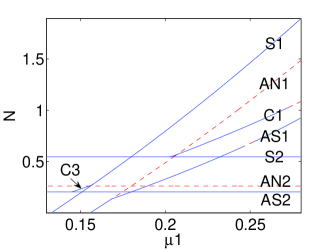
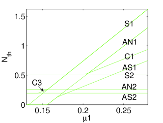
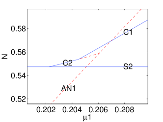
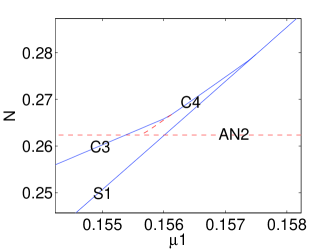
Figure 8: (Color online) Top panel: the norm of the numerical (left) and approximate (right) stationary solutions to Eq.(1) with the self-repulsive nonlinearity ($\sigma=1$) as a function of $\mu_{1}$ for $\mu_{2}=0.18$. Bottom panel: blowups of segments of the top left panel where bifurcations of two-components solutions happen.

The remaining three regimes and the bifurcation scenarios predicted by the finite-mode approximation are shown in the left and right panels of Fig. 9. The top panel corresponds to the case of $\omega_{1}<\mu_{2}<\mu_{2}^{\mathrm{(cr)}}$, when the absence of asymmetric branch AS2 (upon merging into which, C3 would terminate) prevents the existence of the pair of two-component branches, C3 and C4, while C1 and C2 persist in this case. In the middle panel, corresponding to $\omega_{0}<\mu_{2}<\omega_{1}$, we observe that only S2 survives among the single-mode branches in field $v$, and none of the combined solutions is present. Finally, as might be naturally expected, no branches with $u=0$ exist at $\mu_{2}<\omega_{0}$, hence no bifurcations of two-component branches are possible (i.e., we get back to the one-component picture). In all these three cases, we observe good agreement of the numerically found scenarios with the bifurcation diagrams predicted by the two-mode approximation, which are displayed in the right panels.

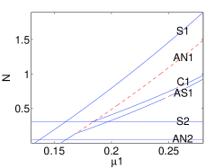
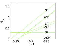
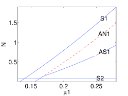
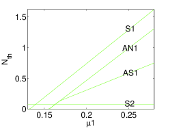
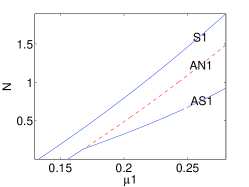
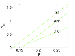
Figure 9: (Color online) The norm of the numerical (left) and semi-analytical (right) solutions of Eq. (1) for the self-repulsive nonlinearity ($\sigma=1$) as a function of $\mu_{1}$, with $\mu_{2}=0.16$ (top), $\mu_{2}=0.14$ (middle), $\mu_{2}=0.12$ (bottom). The notation is the same as in Fig. 8.

An interesting difference between the self-focusing and defocusing nonlinearities is that, as seen in both Figs. 8 and 9, in the latter case the bifurcating branches (such as AS1 and C1) may become unstable due to a Hamiltonian Hopf bifurcation and the resulting oscillatory instability associated with a quartet of complex eigenvalues. This instability, which was known in the single-component setting (see, e.g.,, Ref. todd ), affects a short dashed (red-colored) interval within branches AS1 and C1 in Figs. 8 and 9. An example of such an unstable configuration and the associated spectral plane of the stability eigenvalues are shown in Fig. 10.

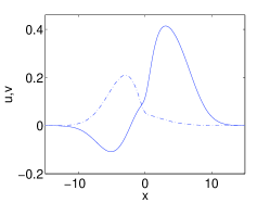
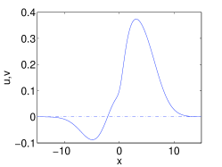
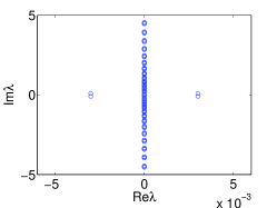
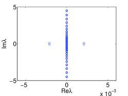
Figure 10: (Color online) Profiles of wave functions $u$ and $v$ (solid and dash-dotted lines, respectively, in the top panel), and the respective stability eigenvalues (bottom) corresponding to solutions of types C1 at $\mu_{2}=0.276$ (left), and AS1 at $\mu_{2}=0.25$ (right). Branches C1 and AS1 are shown in Fig. 8. The existence of the quartet of complex stability eigenvalues implies the oscillatory instability of the solution.

Finally, we examine the dynamical evolution of the unstable two-component solutions that were revealed by the above analysis. The evolution of a typical unstable solution belonging to branches C2 (left panels) and C4 (right panels) past the bifurcation points (at which branches C1 and C3 emerge, respectively) is shown for the cases of the self-attractive and self-repulsive nonlinearity in Figs. 11 and 12. The main dynamical feature apparent in the instability evolution is the growth of the asymmetry of the wave functions between the two potential wells. In each case, this leads to different wells trapping more atoms (or more power, in terms of optics) in each one of the two components. For instance, in the left panel of Fig. 11, we observe, at $t\approx 300$, that the first component features a larger norm in the right well, while the second component – in the left one. Due to the Hamiltonian nature of the system, the two components do not settle down into a static asymmetric configuration, but rather oscillate between the two mirror-image asymmetric states, which (as stationary solutions) are generated by the pitchfork bifurcation. In particular, the instability of branch C2 causes oscillations around the two asymmetric states belonging to branches C1, and, similarly, the evolution of C4 leads to oscillations around the two states of type C3.

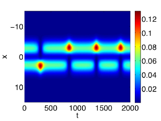
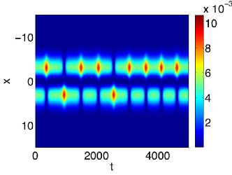
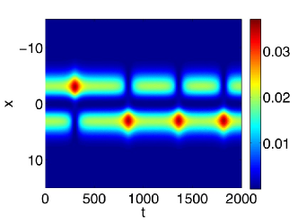
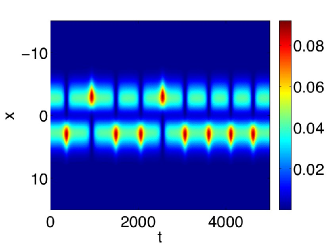
Figure 11: (Color online) Spatiotemporal contour plots of the densities, $|u|^{2}$ and $|v|^{2}$, of unstable two-components (combined) solutions for the self-attractive nonlinearity ($\sigma=-1$). The left and right panels depict the simulated evolution of wave functions $u$ (top) and $v$ (bottom) in the unstable solutions of types C2 and C4, respectively, from Fig. 1.

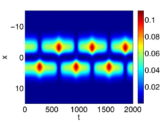
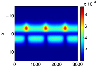
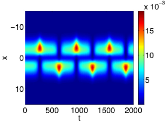
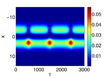
Figure 12: (Color online) The same as in Fig. 12, but for the self-repulsive nonlinearity ($\sigma=1$). Left and right panels show the evolution in the case of the unstable solutions of types C2 and C4, respectively, from Fig. 8.

IV Conclusions

In this work, we have presented the phenomenology and full bifurcation analysis of two-component mixtures trapped in the DWP (double-well potential). The model is of straightforward interest to BEC and nonlinear optics (in the spatial domain). In our analytical considerations we have developed a two-mode (in terms of each component) approximation, that reduces the search for stationary states to solving a set of algebraic equations. The bifurcation diagrams obtained in this approximation, which involve all relevant solutions, have been verified by the comparison with their counterparts produced by the numerical solution of the full PDE model. The novel feature of the two-component setting, in comparison with its previously explored single-component counterpart, is the existence of numerous branches of the “combined” solutions that involve both components. These branches emerge from and merge into previously known single-component ones. The new branches may combine a symmetric field profile in one component and an anti-symmetric one in the other. In addition, asymmetric (in both components) combined branches have been found too; they emerge from the symmetric/anti-symmetric two-component states via pitchfork bifurcations, similar to how bifurcations of the same type give rise to asymmetric solutions in single-component models. The stability analysis of all the considered branches confirms expectations suggested by the general bifurcation theory, according to which the pitchfork destabilizes the previously stable “parent” branch, from which the two new ones (mirror images of each other) emerge. Direct numerical simulations of unstable symmetric two-component solutions (past the bifurcation point) indicate that the instability leads (quite naturally) to oscillations around the asymmetric profiles emerging from the bifurcation.

This study can be extended in several directions. On the one hand, it would be interesting to address this two-component setting using the phase-space analysis, similarly to how it was done in smerzi . Another possibility is to develop an extension of the one-component shooting method of zezy1 to find an entire set of stationary solutions of the system; this is similar to what has been done for two-component optical lattices in the interesting, very recent work of zezy3 (also, many of the relevant solutions appear quite similar to the ones obtained herein). It should nevertheless be mentioned, in connection to zezy3 , that in the present problem there is a straightforward linear limit whose eigenfunctions/eigenvalues allow us to construct all the possible solutions that emerge in the presence of nonlinearity. It may also be interesting to consider the two-component double-well system in the presence of a spatially modulated nonlinearity in the spirit of Ref. zezy2 ; note that both our semi-analytical and numerical approach could be directly adapted to that setting. Finally, it would be particularly interesting to extend this analysis to a four-well, two-dimensional setting (which may naturally emerge from a combination of a magnetic trap with a square 2D optical lattice in a “pancake-shaped” BEC). Numerous additional solutions and a much richer phenomenology may be expected in the latter case. Some of these directions are currently under study.

References

- (1) C. Sulem, P. L. Sulem, The Nonlinear Schrödinger Equation, (Springer-Verlag, New York, 1999).
- (2) M. J. Ablowitz, B. Prinari, A.D. Trubatch, Discrete, Continuous Nonlinear Schrödinger systems (Cambridge University Press, Cambridge, 2003).
- (3) L. P. Pitaevskii, S. Stringari, Bose-Einstein Condensation, Oxford University Press (Oxford, 2003).
- (4) C. J. Pethick, H. Smith, Bose-Einstein condensation in dilute gases, Cambridge University Press (Cambridge, 2002).
- (5) F. Dalfovo, S. Giorgini, L. P. Pitaevskii, S. Stringari, Rev. Mod. Phys. 71, 463 (1999); P. G. Kevrekidis, D. J. Frantzeskakis, Mod. Phys. Lett. B 18, 173 (2004); V. V. Konotop, V. A. Brazhnyi, Mod. Phys. Lett. B 18 627, (2004).
- (6) Yu. S. Kivshar, G. P. Agrawal, Optical Solitons: From Fibers to Photonic Crystals, Academic Press (San Diego, 2003).
- (7) D. N. Christodoulides, F. Lederer, Y. Silberberg, Nature 424, 817 (2003); J. W. Fleischer, J. Fleischer, G. Bartal, O. Cohen, T. Schwartz, O. Manela, B. Freedman, M. Segev, H. Buljan, N. Efremidis, Opt. Exp. 13, 1780 (2005).
- (8) M. Albiez, R. Gati, J. Fölling, S. Hunsmann, M. Cristiani, M. K. Oberthaler, Phys. Rev. Lett. 95, 010402 (2005).
- (9) S. Raghavan, A. Smerzi, S. Fantoni, S. R. Shenoy, Phys. Rev. A 59, 620 (1999); S. Raghavan, A. Smerzi, V. M. Kenkre, Phys. Rev. A 60, R1787 (1999); A. Smerzi, S. Raghavan, Phys. Rev. A 61, 063601 (2000).
- (10) E. A. Ostrovskaya, Y. S. Kivshar, M. Lisak, B. Hall, F. Cattani, D. Anderson, Phys. Rev. A 61, 031601 (R) (2000).
- (11) K. W. Mahmud, J. N. Kutz, W. P. Reinhardt, Phys. Rev. A 66, 063607 (2002).
- (12) V. S. Shchesnovich, B.A. Malomed, R. A. Kraenkel, Physica D 188, 213 (2004).
- (13) D. Ananikian, T. Bergeman, Phys. Rev. A 73, 013604 (2006).
- (14) P. Ziń, E. Infeld, M. Matuszewski, G. Rowlands, M. Trippenbach, Phys. Rev. A 73, 022105 (2006).
- (15) T. Kapitula, P. G. Kevrekidis, Nonlinearity 18, 2491 (2005).
- (16) G. Theocharis, P. G. Kevrekidis, D. J. Frantzeskakis, P. Schmelcher, Phys. Rev. E 74, 056608 (2006).
- (17) D. R. Dounas-Frazer, A. M. Hermundstad, L. D. Carr, Phys. Rev. Lett. 99 (2007) 200402.
- (18) G. Watanabe, C. J. Pethik, Phys. Rev. A 76 (2007) 021605 (R).
- (19) V. I. Yukalov, E. P. Yukalova, Phys. Rev. A 73 (2006) 022335.
- (20) A. Gubeskys, B. A. Malomed, Phys. Rev. A 75, 063602 (2007).
- (21) M. Matuszewski, B. A. Malomed, M. Trippenbach, Phys. Rev. A 75 (2007) 063621.
- (22) A. Gubeskys, B. A. Malomed, Phys. Rev. A, in press.
- (23) C. Cambournac, T. Sylvestre, H. Maillotte , B. Vanderlinden, P. Kockaert, Ph. Emplit, M. Haelterman, Phys. Rev. Lett. 89 (2002) 083901.
- (24) P. G. Kevrekidis, Z. Chen, B. A. Malomed, D. J. Frantzeskakis, M. I. Weinstein, Phys. Lett. A 340 (2005) 275.
- (25) M. Ornigotti, G. Della Valle, D. Gatti, S. Longhi, Phys. Rev. A 76 (2007) 023833.
- (26) N. Akhmediev, A. Ankiewicz, Phys. Rev. Lett. 70 (1993) 2395; P. L. Chu, B. A. Malomed, G. D. Peng, J. Opt. Soc. Am. B 10 (1993) 1379; J. M. Soto-Crespo, N. Akhmediev, Phys. Rev. E 48 (1993) 4710 (1993); B. A. Malomed, I. Skinner, P. L. Chu, G. D. Peng, Phys. Rev. E 53 (1996) 4084.
- (27) W. Mak, B. A. Malomed, P. L. Chu, J. Opt. Soc. Am. B 15 (1998) 1685; Y. J. Tsofe, B. A. Malomed, Phys. Rev. E 75 (2007) 056603.
- (28) W. Mak, B. A. Malomed, P. L. Chu, Phys. Rev. E 55 (1997) 6134.
- (29) L. Albuch, B. A. Malomed, Math. Comp. Simul. 74 (2007) 312.
- (30) A. Sigler, B. A. Malomed, Physica D 212 (2005) 305.
- (31) N. N. Akhmediev, A. V. Buryak, J. Opt. Soc. Am. 11 (1994) 804.
- (32) A. Gubeskys, B. A. Malomed, Eur. Phys. J. 28 (2004) 283.
- (33) A. Sigler, B. A. Malomed, D. V. Skryabin, Phys. Rev. E 74 (2006) 066604.
- (34) E. W. Kirr, P. G. Kevrekidis, E. Shlizerman, M. I. Weinstein, arXiv:nlin/0702038, SIAM J. Math. Anal, in press.
- (35) A. Sacchetti, SIAM J. Math. Anal. 35 (2004) 1160 (2004).
- (36) D. Bambusi, A. Sacchetti, arXiv:math-ph/0608010.
- (37) K. M. Mertes, J. Merrill, R. Carretero-González, D. J. Frantzeskakis, P. G. Kevrekidis, D. S. Hall, Phys. Rev. Lett. 99, 190402 (2007)
- (38) Z. Chen , J. Yang, A. Bezryadina, I. Makasyuk, Opt. Lett. 29 (2004) 1656.
- (39) S. V. Manakov, Zh. Eksp. Teor. Fiz. 65 (1973) 505 [Soviet Physics-JETP Vol. 38 (1974) 248 ].
- (40) G. L. Alfimov, D. A. Zezyulin, Nonlinearity 20 (2007) 2075.
- (41) H.A. Cruz, V.A. Brazhnyi, V.V. Konotop, G.L. Alfimov and M. Salerno, Phys. Rev. A 76, 013603 (2007).
- (42) D. A. Zezyulin, G. L. Alfimov, V. V. Konotop, V. M. Perez-Garcia, Phys. Rev. A 76 (2007) 013621.