Optimized Schwarz preconditioning for SEM based magnetohydrodynamics

Summary. A recent theoretical result on optimized Schwarz algorithms demonstrated at the algebraic level enables the modification of an existing Schwarz procedure to its optimized counterpart. In this work, it is shown how to modify a bilinear FEM based Schwarz preconditioning strategy originally presented in Fis (97) to its optimized version. The latter is employed to precondition the pseudo–Laplacian operator arising from the spectral element discretization of the magnetohydrodynamic equations in Elsässer form.

1 Introduction

This work concerns the preconditioning of a pseudo–Laplacian operator associated with the saddle point problem arising at each time-step in a spectral element based adaptive MHD solver. The approach proposed herein is a modification of the method developed in Fis (97) where an overlapping Schwarz preconditioner was constructed using a low oder discretization. The latter approach is based on the spectral equivalence between finite-elements and spectral elements CHQZ (07); Kim (06). The finite-element blocks, representing the additive Schwarz, are replaced by so called optimized Schwarz blocks SCGT07a . Two types of meshes, employed to construct the $\mathbb{Q}_{1}$ block preconditioning are investigated. The first one is cross shaped and shows good behavior for additive Schwarz (AS) and restricted additive Schwarz (RAS). However improved convergence rates of the optimized RAS (ORAS) version are completely dominated by the corner effects CNN (06). Opting for a second grid that includes the corners seems to correct this issue. For the zeroth order optimized transmission condition (O0) an exact tensor product form is available while for the O2 version a slight error is introduced in order to preserve the properties of the operators and enable the use of fast diagonalization techniques introduced for spectral elements in Cou (95). It is shown how to modify trivially an existing fast-diagonalization procedure and numerical experiments demonstrate the efficiency of the modification.

2 Governing equations and discretization

For an incompressible fluid with constant mass density $\rho_{0}$, the magnetohydrodynamic (MHD) equations are:

$$\partial_{t}{{\bf u}}+{{\bf u}}\cdot{{\nabla}}{{\bf u}}=-{{\nabla}}p+{bfj}\times{\bf b}+\nu\nabla^{2}{{\bf u}},$$ (1)

$$\partial_{t}{{\bf b}}={{\nabla}}\times({\bf u}\times{\bf b})+\eta\nabla^{2}{{\bf b}}$$ (2)

$${{\nabla}}\cdot{{\bf u}}=0,\hskip 14.45377pt{{\nabla}}\cdot{{\bf b}}=0$$ (3)

where ${{\bf u}}$ and ${\bf b}$ are the velocity and magnetic field (in Alfvén velocity units, ${\bf b}={\bf B}/\sqrt{\mu_{0}\rho_{0}}$ with ${\bf B}$ the induction and $\mu_{0}$ the permeability); $p$ is the pressure divided by the mass density, and $\nu$ and $\eta$ are the kinematic viscosity and the magnetic resistivity. In Elsässer form, the equations are Els (50):

$$\partial_{t}{\bf Z}^{\pm}+{\bf Z}^{\mp}\cdot{{\nabla}}{\bf Z}^{\pm}+{{\nabla}}p-\nu^{\pm}\nabla^{2}{\bf Z}^{\pm}-\nu^{\mp}\nabla^{2}{\bf Z}^{\mp}=0$$ (4)

$${{\nabla}}\cdot{\bf Z}^{\pm}=0\,,$$ (5)

with ${\bf Z}^{\pm}={\bf u}\pm{\bf b}$ and $\nu^{\pm}=\frac{1}{2}(\nu\pm\eta)$. The velocity ${\bf u}$ and magnetic field ${\bf b}$ can be recovered by expressing them in terms of ${\bf Z}^{\pm}$. Since all time-scales are of interest, an explicit second order Runge-Kutta scheme is applied to discretize the time-derivative of the above system while, for the spatial part, a $\mathbf{P}_{N}-\mathbf{P}_{N-2}$ spectral element formulation was chosen to prevent the excitation of spurious pressure modes using the spaces

$$\mathbf{U}_{{\bf\gamma}} \mathbin{:=}\left\{{\bf w}=\sum_{\mu=1}^{d}w^{\mu}{\vec{e}}^{\>\mu}\,\left\bracevert w^{\mu}\in\mathbf{H}^{1}({D})\;\forall\mu\;\&\;{\bf w}={\bf\gamma}\;{\rm on}\;\partial D\right.\right\}$$ (6)

$$\mathbf{H}^{1}(D) \mathbin{:=}\left\{f\,\left\bracevert f\in\mathbf{L}_{2}(D)\;\&\;\partial_{x^{\mu}}f\in\mathbf{L}_{2}(D)\;\forall\mu\right.\right\}\,,$$ (7)

with ${\bf w}={\bf u},\,{\bf b}$, ${\bf Z}^{\pm}$, $p$ and their test functions, ${\bf\zeta}^{\pm}$ and $q$ restricted to finite–dimensional subspaces of these spaces:

$${\bf Z}^{\pm}\in\mathbf{U}^{N}\;\;\;=\mathbf{U}_{{\bf Z}_{0}}\;\bigcap\;\mathbf{P}_{N}, {\bf\zeta}^{\pm}\in\mathbf{U}_{0}^{N}\;\;\;\;=\mathbf{U}_{{\bf 0}}\;\bigcap\;\mathbf{P}_{N},$$

$$p,q\in\mathbf{Y}^{N-2}=\mathbf{L}_{2}(D)\;\bigcap\;\mathbf{P}_{N-2}$$

see for instance MPR (92); Fis (97). The basis for the velocity expansion in $\mathbf{P}_{N}$ is the set of Lagrange interpolating polynomials on the Gauss-Lobatto-Legendre (GL) quadrature nodes, and the basis for the pressure is the set of Lagrange interpolants on the Gauss-Legendre (G) quadrature nodes. In the spectral element method formalism, the domain, $\mathbf{D}$, is composed of a union of non-overlapping subdomains, or elements, $\mathbf{E}_{k}$: $\mathbf{D}=\bigcup_{k=1}^{K}\mathbf{E}_{k}$, and functions in $\mathbf{U}^{N}$ and $\mathbf{Y}^{N-2}$ are represented as expansions in terms of tensor products of basis functions within each subdomain. The complete discretization at each stage is:

$$\hat{{\boldsymbol{Z}}}_{j}^{\pm}=\hat{{\boldsymbol{Z}}}_{j}^{\pm,n}-\frac{1}{k}\Delta t\;\mbox{$\textbf{M}$}^{-1}(\mbox{$\textbf{M}$}\mbox{$\textbf{C}$}^{\mp}\hat{{\boldsymbol{Z}}}_{j}^{\pm}-\mbox{$\textbf{D}$}^{\rm T}_{j}\hat{{\boldsymbol{p}}}^{\pm}+\nu_{\pm}\mbox{$\textbf{L}$}\hat{{\boldsymbol{Z}}}_{j}^{\pm}+\nu_{\mp}\mbox{$\textbf{L}$}\hat{{\boldsymbol{Z}}}_{j}^{\mp}).$$ (8)

We require that each Runge-Kutta stage obeys (5) in its discrete form, so multiplying (8) by $\mbox{$\textbf{D}$}_{j}$, summing, and setting the term $\mbox{$\textbf{D}$}^{j}\hat{{\boldsymbol{Z}}}_{j}^{\pm}=0$ leads to the following pseudo–Poisson equation for the pressures, $\hat{{\boldsymbol{p}}}^{\pm}$:

$$\mbox{$\textbf{D}$}^{j}\mbox{$\textbf{M}$}^{-1}\mbox{$\textbf{D}$}^{\rm T}_{j}\hat{{\boldsymbol{p}}}^{\pm}=\mbox{$\textbf{D}$}^{j}{\boldsymbol{g}}_{j}^{\pm}\,,$$ (9)

where the quantity

$${\boldsymbol{g}}_{j}^{\pm}=\frac{1}{k}\Delta t\;\mbox{$\textbf{M}$}^{-1}(\mbox{$\textbf{M}$}\mbox{$\textbf{C}$}^{\mp}\hat{{\boldsymbol{Z}}}_{j}^{\pm}+\nu_{\pm}\mbox{$\textbf{L}$}\hat{{\boldsymbol{Z}}}_{j}^{\pm}+\nu_{\mp}\mbox{$\textbf{L}$}\hat{{\boldsymbol{Z}}}_{j}^{\mp})-\hat{{\boldsymbol{Z}}}_{j}^{\pm,n}.$$

is the remaining inhomogeneous contribution (see RPM (07)). More details on the various operators can be found in DFM (02). Equation (9) is solved using a preconditioned iterative Krylov method.

3 From classical to optimized Schwarz

The principle behind optimized Schwarz methods consists into replacing the Dirichlet transmission condition present in the classical Schwarz approach by a more general boundary condition. This idea was first analyzed by Lions in Lio (88) where a Robin condition was introduced. The latter contained a positive parameter that could possibly be used to enhance convergence. However, until recently, it was not clear how to define optimally that parameter for the new conditions at the interfaces between subdomains. Optimized Schwarz methods are derived from a Fourier analysis of the continuous elliptic partial differential equation, see for instance Gan (06) and references therein. Starting from the problem stated at the continuous level, suppose that a linear elliptic operator $\mathcal{L}$ with forcing $f$ and boundary conditions $\mathcal{P}$ needs to be solved on $\mathbf{D}$. An algorithm that can be employed to solve the global problem $\mathcal{L}u=f$ is

$$\mathcal{L}u^{n+1}_{i} =f\;\;\mbox{in $\mathbf{\bar{E}}_{i}$}$$

$$\mathcal{P}(u^{n+1}_{i}) =g\;\;\mbox{on $\partial\mathbf{D}\cap\mathbf{\bar{E}}_{i}$}$$ (10)

$$u^{n+1}_{i} =u^{n}_{j}\;\;\mbox{on $\Gamma_{ij}$}$$

where the sequence with respect to $n$ will be convergent for any initial guess $u^{0}$ with

$$\Gamma_{ij}\equiv\partial\mathbf{\bar{E}}_{i}\cap\mathbf{\bar{E}}_{j}\neq\{\emptyset\}.$$

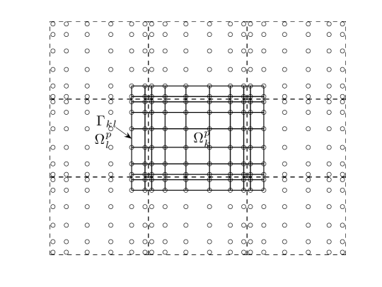
Figure 1: One overlapping element

This is none other than the classical Schwarz algorithm at the continuous level corresponding to RAS at the matrix level. In Fig. 1, $\Omega^{p}_{k}$ represents the quadrangulation of the overlapping domain $\mathbf{\bar{E}}_{k}$. The optimized version of the above algorithm replaces the transmission conditions between subdomains by

$$\begin{array}[]{rcll}\tilde{\mathcal{B}}_{ij}u^{n+1}_{i}&=&\tilde{\mathcal{B}}_{ij}u^{n}_{j};\;\mbox{on $\Gamma_{ij}$}\\ \end{array}$$

where $\tilde{\mathcal{B}}_{ij}$ makes each subproblem well posed and can be a function of optimizable parameters: the algorithm, like in the classical case, converges to the solution of $\mathcal{L}u$ with $\mathcal{P}(u)=g$ on $\mathbf{D}$. The discrete algebraic version is

$$\left(\begin{array}[]{cc}A^{k}_{ii}&A^{k}_{i\Gamma}\\ C^{k}_{\Gamma i}&C^{k}_{\Gamma\Gamma}\end{array}\right)\left(\begin{array}[]{c}u^{k}_{i}\\ u^{k}_{\Gamma}\end{array}\right)^{n+1}=\left(\begin{array}[]{c}f^{k}_{i}\\ C^{k}(u_{\partial\Omega^{p}_{k}})^{n}\end{array}\right)$$

with $C^{k}_{\Gamma i}$, $C^{k}_{\Gamma\Gamma}$ and $C$ corresponding to the the discrete expressions of the new transmission conditions. At this point notice that $A^{k}_{ii}$ is exactly the same block as in the original Schwarz algorithm. A simple (block) Gaussian elimination leads to the following preconditioned system

$$\{I-\sum^{K}_{j,k=1}(\tilde{R}^{k})^{T}\tilde{B}_{kj}R^{j}\}u=\sum^{K}_{k=1}(\tilde{R}^{k})^{T}(\tilde{A}^{k}_{ii})^{-1}R^{k}f$$ (11)

with $\tilde{A}^{k}_{ii}=A^{k}_{ii}-A^{k}_{i\Gamma}(C^{k}_{\Gamma\Gamma})^{-1}C^{k}_{\Gamma i}$. Thus, the optimized restricted additive Schwarz preconditioning is expressed as $P^{-1}_{ORAS}\equiv\sum^{K}_{k=1}(\tilde{R}^{k})^{T}(\tilde{A}^{k}_{ii})^{-1}R^{k}$. The above results are completely algebraic and independent of the underlying space discretization method. The complete proof in the additive and multiplicative case with and without overlap can be found in SCGT07a . In the case of two subdomains it can be shown that the optimal transmission operator is the Schur complement SCGT07b . Also in weighted residual techniques the artificial boundary conditions should be properly weighted.

4 $Q_{1}$ formulation and optimized Schwarz

The $Q_{1}$ formulation for the Schwarz algorithm can be found in (cite). We merely express here the changes necessary in order to obtain an optimized version. First, the overlap depicted in Fig. 1 is the minimal one. Secondly, the normal or tangential derivatives expressions at the boundaries must not involve more than $2$ points. Including more would destroy the optimized iterates as mentioned in SCGT07a (remark $1$). Both requirements are satisfied by the $Q_{1}$ FEM formulation naturally.

It is important to handle the assembly of the Q1 operators correctly at the endpoints. Thus we build our reference interval on the extended grid to include one additional node at each end of the interval. We then begin the assembly (direct stiffness summation) starting at the second node on the left, and continuing until the second-to-last node on the right. In this way, the negative–sloping linear FEM shape function on the left–most subinterval and the positive–sloping shape function on the rightmost subinterval are not included in the assembly. The general idea is illustrated in figure 2.

Figure 2: Schematic of Q1 assembly. The left– and right–most dashed shape functions are not included in the assembly.

We can define for the linear problem in equation (3) a general transmission condition SCGT07a between each element

$$\left[\frac{\partial u_{j}}{\partial{\bf n}}+T(u_{j},p,q,\tau)\right]^{n+1}_{\Gamma_{ij}}=\left[\frac{\partial u_{i}}{\partial{\bf n}}+T(u_{j},p,q,\tau)\right]^{n}_{\Gamma_{ij}}$$

where the interface blocks $T(u_{j},p,q,\tau)\equiv pu_{j}-q\frac{\partial^{2}u_{j}}{\partial\tau^{2}}$, define a transmission condition of order $2$ with two parameters, $p$ and $q$, specified in Gan (06), and also provided for completeness in table 1. In general, $p$ and $q$ are different depending on whether there is overlap, but here we consider only the case of finite overlap.

	$p$	$q$
OO0, overlap $Ch$	$2^{-1/3}(k^{2}_{\min}+\eta)^{1/3}(Ch)^{-1/3}$	0
OO2, overlap $Ch$	$2^{-3/5}(k_{\min}^{2}+\eta)^{2/5}(Ch)^{-1/5}$	$2^{-1/5}(k_{\min}^{2}+\eta)^{-1/5}(Ch)^{3/5}$

Table 1: Choices for the parameters $p$ and $q$ used in the interface blocks. OOj stands for optimized of order j.

4.1 FDM

When rectangular elements are considered a fast diagonalization method (FDM) (e.g., Cou (95)) can be used to invert the optimized $Q_{1}$ blocks. The number of operations required to invert $N^{d}\times N^{d}$ matrix using such a technique is $O(N^{d+1})$ and the application of the inverse is performed using efficient tensor products in $O(N^{d})$ operations. We propose the form

$$\tilde{A}_{ii}=(M+T_{0}q)\otimes(K+T_{0}p)+(K+T_{o}p)\otimes(M+T_{0}q)$$ (12)

as the optimized block matrix where $T_{0}$ is a matrix almost completely filled with zeros with the exception of the entries $(1,1)$ and $(N,N)$ which are set to $1$. This form implements the weak form of the transmission conditions, Equation (4), directly in the optimized block, $\tilde{A}_{ii}$. Notice that in order for the fast diagonalization technique to be applicable, the coefficients $p$ and $q$ must be constant on their face. The modified matrix $M+T_{o}q$ is still symmetric and positive definite while the matrix $K+T_{o}p$ is still symmetric. This enables the use of the modified mass matrix in an inner product and the simultaneous diagonalization of both tensors. When $q=0$ the proposed formula is exact; however, when $q\neq 0$ a slight error is made at the corners. If the quantity $(T_{0}p)\otimes(T_{0}q)$ was removed then the expression in the $O2$ would also be exact.

5 Numerical experiments

We have implemented the RAS preconditioner described above in the MHD code. This version allows for variable overlap of the extended grid. The ORAS counterpart has also been implemented as described by starting from the RAS, and for comparison, we can use a high-order block Jacobi (BJ) method as well. We consider first tests of a single pseudo–Poisson solve. We use a periodic grid of $E=8\times 8$ elements, and iterate using BiCGStab until the residual is $10^{-8}$ times that of the initial residual. The extended grid overlap is $2$, and the initial starting guess for the Krylov method is composed of random noise. The first test, uses non-FDM preconditioners to investigate the effect of including corner transfers on the optimization. The results are presented in Fig. 3, in which we consider only the O0 optimization. Note that even thought the RAS is much less sensitive to the corner communication, especially at higher $N_{v}$, the O0 with corners requires fewer iterations. Clearly, corner communication is crucial to the proper functioning of the optimized methods.

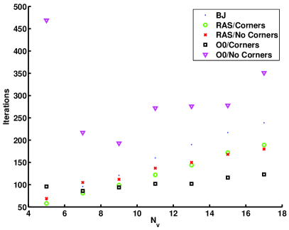
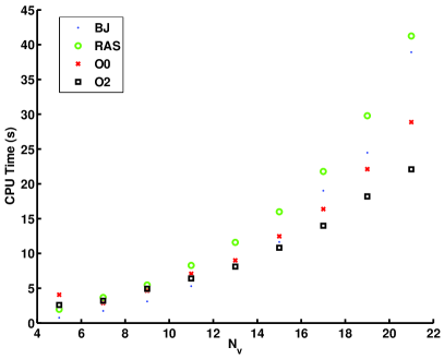
Figure 3: left: Plot of iteration count vs GLL-expansion node number for different preconditioners with and without corner communication on an $8\times 8$ element grid. right: Comparison of of CPU time vs. GLL-expansion node number of FDM-based preconditioners with corner communication on a $16\times 16$ element grid.

In the next experiment, all the parameters are maintained except we use a grid of $E=16\times 16$ elements together with the FDM version of the preconditioners to investigate performance. These results are presented on the right-most figure of Fig. 3.

6 Conclusions and future directions

It is shown that a simple modification of a RAS in a low order FDM based preconditioning of the the pseudo–Laplacian operator can reduce the time to solution by up to a factor of two for high order GLL expansions. Also, as expected from the work of CNN (06), we find that the cross form of the subdomains is not suitable as is for the optimized version of the algorithm: corners need to be included. Upcoming work will concern the inclusion of a coarse solver in this approach and a treatment for non-conforming elements.

Acknowledgments

The third author was upported by Korea’s Research Foundation under grant number KRF-2005-070-C00017. The first author is grateful for the support provided by the BK21 program. NCAR is supported by the National Science Foundation.

References

- CHQZ [07] C.G. Canuto, M.Y. Hussaini, A. Quarteroni, and T.A. Zang. Spectral methods Evolution to Complex Geometries and Applications to Fluid Dynamics. Scientific Computation. Springer Verlag, 2007.
- CNN [06] Chokri Chniti, Frédéric Nataf, and Francis Nier. Improved interface condition for 2d domain decomposition with corner : a theoretical determination. Technical Report hal-00018965, Hyper articles en ligne, 2006.
- Cou [95] Wouter Couzy. Spectral element discretization of the unsteady Navier-Stokes equations and its iterative solution on parallel computers. PhD thesis, École Polytechnique Fédérale de Lausanne, 1995.
- DFM [02] M.O. Deville, P. F. Fischer, and E. H. Mund. High-Order Methods for Incompressible Fluid Flow. Cambridge University Press, 2002.
- Els [50] W.M. Elsässer. The hydromagnetic equations. Physical Review, 79:183, 1950.
- Fis [97] P.F. Fischer. An overlapping schwarz method for spectral element solution of the incompressible navier-stokes equations. Journal of Computational Physics, 133:84–101, 1997.
- Gan [06] Martin J. Gander. Optimized schwarz methods. SIAM Journal on Numerical Analysis, 44(2):699–731, 2006.
- Kim [06] Sang Dong Kim. Piecewise bilinear preconditioning for high-order finite element methods. Electronic Transactions on Numerical Analysis, 2006. to appear.
- Lio [88] P.-L. Lions. On the Schwarz alternating method. I. In R. Glowinski, G. H. Golub, G. A. Meurant, and J. Périaux, editors, First International Symposium on Domain Decomposition Methods for Partial Differential Equations, pages 1–42, Philadelphia, PA, 1988. SIAM.
- MPR [92] Y. Maday, A.T. Patera, and E.M. Rønquist. The - method for the approximation of the stokes problem. Technical report, Pulications du Laboratoire d’Analyse Numrique, Universit Pierre et Marie Curie, 1992.
- RPM [07] D. Rosenberg, A. Pouquet, and P. D. Mininni. Adaptive mesh refinement with spectral accuracy for magnetohydrodynamics in two space dimensions. New Journal of Physics, 9(304), 2007.
- [12] A. St-Cyr, M. J. Gander, and S. J. Thomas. Optimized multiplicative, additive, and restricted additive schwarz preconditioning. SIAM Journal on Scientific Computing, 29(6):2402–2425, 2007.
- [13] A. St-Cyr, M. J. Gander, and S. J. Thomas. Optimized restricted additive schwarz. In Olof B. Widlund and D. E. Keyes, editors, Domain Decomposition Methods in Science and Engineering XVI, volume 55 of Lecture Notes in Computational Science and Engineering, pages 213–220. Springer Verlag, 2007.