Note on the ring approximation in nuclear matter

Abstract

The response function to an external prove is evaluated using the ring approximation in nuclear matter. Contrary to what it is usually assumed, it is shown that the summation of the ring series and the solution of the Dyson’s equation are two different approaches. The numerical results exhibit a perceptible difference between both approximations.

The ring approximation is widely used in many nuclear physics problems. It consists of the infinite sum of one particle-one hole bubbles, where the Pauli exchange contribution is neglected fe71 . In fact, the ring approximation is the direct part of the Random Phase Approximation (RPA). By neglecting the exchange terms, the particle-hole series reduces itself to a geometric series, which is easily summed up. As an alternative derivation, it is usually proposed the ring series as the solution of the Dyson’s equation dy49 (see also fe71 ). It has come to us as a surprise the existence of an inconsistency between the interpretation of the ring approximation as a solution of the Dyson’s equation and the explicit evaluation (employing the Goldstone’s rules) of the particle-hole diagrams which originates the ring series. This inconsistency comes into play only when one particle-hole configuration is on the mass shell, for example, when we study the response function. In this contribution we discuss this point and we show that there are two alternative approximations. One is the solution of the plain Dyson’s equation and the other is the summation of the ring diagrams.

Let us consider an arbitrary one-body operator ${\cal O}_{\alpha}$ exciting the nucleus from its ground state $|0>$. The action of ${\cal O}_{\alpha}$ is characterized by the nuclear response function per nuclear volume,

$$S_{\alpha}(q_{0},\mbox{\boldmath$q$})=-\frac{1}{\pi\,\Omega}\ Im<0|{{\cal O}_{\alpha}}^{{\dagger}}G(q_{0}){\cal O}_{\alpha}|0>,$$ (1)

where $q_{0}$ and $q$ are the energy and momentum transfer, respectively and $\Omega$ is the nuclear volume. The nucleon propagator $G(q_{0})$ is given by,

$$G(q_{0})=\frac{1}{q_{0}-H+i\eta}\ -\frac{1}{q_{0}+H+i\eta}\,$$ (2)

being $H$ the nuclear Hamiltonian. As usual $H=T+V$, where $T$ is the kinetic energy and $V$ is the residual interaction. The identity is expressed as,

$$I=\sum_{n}|n><n|,$$ (3)

where $|n>$ represent a compleat set of orthonormal states of $H$. By inserting the identity twice in Eq. (1), we have,

$$S_{\alpha}(q_{0},\mbox{\boldmath$q$})=\frac{1}{\Omega}\,\sum_{n}\;|<n|{\cal O}_{\alpha}|0>|^{2}\,\delta(q_{0}-q_{n}),$$ (4)

where $q_{n}\equiv E_{n}-E_{0}$ ($\hbar=c=1$), and $E_{n}$ are the excitation energies of the eigenstates $|n>$.

In the present contribution we explore three different external proofs,

$${\cal O}_{\alpha}=\sum_{j}\;e^{i\mbox{\boldmath$q$}\cdot\mbox{\boldmath$x$}_{j}}\widetilde{{\cal O}}_{\alpha\,(j)}$$ (5)

with $x_{j}$ denoting the intrinsic coordinate for individual nucleons and the sum $j$ runs over all nucleons. In this equation, $\widetilde{{\cal O}}_{C\,(j)}=1$, $\widetilde{{\cal O}}_{L\,(j)}=\mbox{\boldmath$\sigma$}_{(j)}\cdot\mbox{\boldmath$\hat{q}$}\,\tau_{z\,(j)}$ and $\widetilde{{\cal O}}_{T\,(j)}=\mbox{\boldmath$\sigma$}_{(j)}\times\mbox{\boldmath$\hat{q}$}\,\tau_{z\,(j)}$ which are usually named as the isoscalar central and isovector spin-longitudinal and spin-transversal operators, respectively. The next step is to propose a model for the Hamiltonian. The simplest choice is to keep only the kinetic energy $T$. In this case, the final state is a one particle-one hole excitation as the one drawn in the first diagram in Fig. 1.

Figure 1: Goldstone’s diagrams representing the firsts contributions to the ring approximation. In each diagram an up (down) arrow constitutes a particle (hole), a wavy line is the residual interaction and a dot stand for the external operator. It has been added an horizontal dashed line to indicate the configuration on the mass shell.

Before we show the response function, in Appendix A, it is presented the lowest-order polarization insertion $\Pi^{0}(q_{0},\mbox{\boldmath$q$})$, which is further expressed as the sum of it real and imaginary parts,

$$\Pi^{0}(q_{0},\mbox{\boldmath$q$})\equiv{\cal R}(q_{0},\mbox{\boldmath$q$})+\imath{\cal I}(q_{0},\mbox{\boldmath$q$})$$ (6)

Now the response function to ${\cal O}_{C}$, is,

$$S^{0}_{C}(q_{0},\mbox{\boldmath$q$})={\cal I}$$ (7)

Next, the residual interaction $V$ is incorporated. As a model for $V$, we use the one given in Eq. (21), which can be rewritten as a sum of a isoscalar central and isovector spin–longitudinal and spin–transversal terms (see Eq. (23)). One way of taking care of the residual interaction is by means of the Dyson’s equation, where a higher-order polarization insertion is obtained as,

$$\Pi^{Dys}(q_{0},\mbox{\boldmath$q$})=\Pi^{0}(q_{0},\mbox{\boldmath$q$})+\Pi^{0}(q_{0},\mbox{\boldmath$q$})\,V(q)\,\Pi^{Dys}(q_{0},\mbox{\boldmath$q$}).$$ (8)

In this equation the Pauli exchange terms have been already neglected. For this reason, this is an algebraic equation which solution is the sum of a geometric series in $V\,\Pi^{0}$,

$$\Pi^{Dys}=\frac{\Pi^{0}}{1-V\,\Pi^{0}}.$$ (9)

Using the solution of the Dyson’s equation a new response function is obtained. This is done by replacing ${\cal I}$ in Eq. (7) by $Im\Pi^{Dys}$,

$$S^{Dys}_{C\,(L,T)}(q_{0},\mbox{\boldmath$q$})=\frac{\cal I}{(1-{{\cal V}_{C\,(L,T)}\,\cal R})^{2}+({\cal V}_{C\,(L,T)}\,{\cal I})^{2}}.$$ (10)

The Eq. (9) is usually interpreted as the sum of a series of one particle-one hole bubbles. The firsts terms to this series are shown in Fig. 1. In these diagrams, a horizontal dashed-line indicates that this configuration is on the mass shell. It is interesting to analyze each term in the series separately, we expand Eq. (9),

$$\frac{\Pi^{0}}{1-V\,\Pi^{0}}=\Pi^{0}(1+V\,\Pi^{0}+(V\,\Pi^{0})^{2}+\ldots),$$ (11)

by taking the imaginary part of this sum, we have,

$$Im(\Pi^{0}) = {\cal I}$$

$$Im(\Pi^{0}V\Pi^{0}) = 2{\cal R}\;V\;{\cal I}$$

$$Im(\Pi^{0}(V\,\Pi^{0})^{2}) = (3{\cal R}^{2}{\cal I}-{\cal I}^{3})\;V^{2}$$ (12)

$$...$$

By inspection of the diagrams in Fig. 1, each term has the following interpretation. The first term (zeroth power in $V$), is the first diagram in the left hand side in this figure. Using the Goldstone’s rules, the analytical expression for a one particle-one hole bubble is given by $\Pi^{0}$. When the bubble is put on it mass shell, we take the imaginary part, ${\cal I}$. The next contribution (first power in $V$), is represented by the second and third diagrams in the same figure. In the second (third) diagram the lower (upper) bubble is on the mass shell. Analytically, the bubble on it mass shell is given by ${\cal I}$, while the other bubble (in the same diagram) is off the mass shell, ${\cal R}$. As both contributions (second and third diagrams) are identical, one has a factor two (i.e., $2{\cal R}\;V\;{\cal I}$). This association between diagrams and physical states fails for the next order contribution. There are three contributions, where the first one is shown in Fig. 1, while the two remainders ones are the same draw, but with the dashed-line (which represents the configuration on it mass shell), in the middle and upper bubble. The first term (i.e., $3{\cal R}^{2}{\cal I}$) is easily interpreted as the sum of these three contributions, where only one bubble at a time is on the mass shell and a factor three results from the equality of the three contributions. However, the ${\cal I}^{3}$-term can not be interpreted: in terms of Eq. (4), all diagrams represent the square of a transition amplitude. To put it in other words, in one diagram only one configuration can be on the mass shell. The ${\cal I}^{3}$-term would imply a diagram with three bubbles simultaneously on the mass shell.

We go back to Eq. (9) where we keep only the terms compatible with Eq. (4),

$$Im(\Pi^{0}) = {\cal I}$$

$$Im(\Pi^{0}V\Pi^{0}) = 2{\cal R}\;V\;{\cal I}$$

$$Im(\Pi^{0}(V\,\Pi^{0})^{2}) = 3{\cal R}^{2}\;V^{2}\;{\cal I}$$

$$...$$

$$Im(\Pi^{0}(V\,\Pi^{0})^{N}) = (N+1)\,{\cal R}^{N}\;V^{N}\;{\cal I}$$ (13)

$$...$$

Each term in this series has a straightforward physical interpretation in terms of the so-called ring diagrams. For this reason, we call the sum as $\Pi^{ring}$. The summation can be easily performed once we notice that,

$$\frac{d}{d({\cal R}\,V)}{\left(\frac{1}{1-{\cal R}\,V}\right)}=1+2{\cal R}\,V+3({\cal R}\,V)^{2}+4({\cal R}\,V)^{3}+\ldots$$ (14)

The final result for the sum is,

$$S^{ring}_{C\,(L,T)}(q_{0},\mbox{\boldmath$q$})=\frac{\cal I}{(1-{{\cal V}_{C\,(L,T)}\,\cal R})^{2}}.$$ (15)

It should be noted that the expression in the left hand side in Eq. (11) is the sum of the series in the right hand side, as long as $|V\,\Pi^{0}|<1$, therefore we have,

$$|V\,\Pi^{0}|=|V|\,\sqrt{{\cal R}^{2}+{\cal I}^{2}}<1,\;as\;{\cal R},{\cal I}\in Re\Rightarrow|V\,{\cal R}|<1\therefore 1-{{\cal V}_{C\,(L,T)}\,\cal R}\neq 0.$$ (16)

Therefore, if the sum in Eq. (11) exists, so does the one in Eq. (15). In order to obtained $S^{Dys}$ and $S^{ring}$, only the imaginary part in Eq. (9) has been evaluated. For completeness, in Appendix A the real parts are also calculated.

As mentioned, we have two different response functions, $S^{Dys}$ and $S^{ring}$. In Fig. 2 we have plotted the numerical result for these two functions, just to show that the difference between them is relevant. It should be emphasized that both response functions are valid solutions for two different ways of dealing with the residual interaction $V$: the $S^{Dys}$-response is the solution of the Dyson’s equation and the $S^{ring}$-response is the sum of the ring diagrams. In the present contribution, it is claimed that the interpretation of the solution of the Dyson’s equation in terms of ring diagrams is wrong, as long as the polarization insertion $\Pi^{0}$ has a not-null imaginary part. In some physical problems, such as the study of zero sound je80 ; st83 or core polarization os93 , only the real part in Eq. (11) is needed. By inspection of Eqs. (24) and (27), it is easy to check that $\Pi^{Dys}=\Pi^{ring}$ when ${\cal I}=0$. In this case, the solution of the Dyson’s equation is also the sum of the ring series. This element could have been misleading in the former interpretation of the solution of the Dyson’s equation. Before we end this paragraphs, another point should be addressed: the interpretation of the solution of the Dyson’s equation in term of Eq. (4). This can be done as follows. We work with the residual interaction,

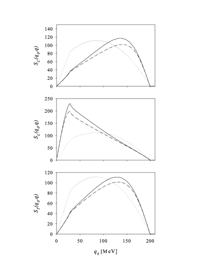
Figure 2: Response function per nuclear volume. In each graph, the dot line represents $S^{0}$, the continuous one $S^{ring}$ and the dash-dot $S^{Dys}$. The momentum transfer by the external operator is chosen as $q=400$ MeV/c, while the parameters entering in $V$ are $f=0.3$, $g^{\prime}=0.5$, $\Lambda_{\pi}=1300$ MeV/c and $\Lambda_{\rho}=1700$ MeV/c. For the Fermi momentum it has been used, $k_{F}=1.36$ 1/fm. The functions $S_{C,\,L\,T}$ are given in units of MeV^-1 fm^-3 $\times 10^{-5}$.

$$V^{Dys}(q_{0},\mbox{\boldmath$q$})=V(q)+V(q)\,\Pi^{0}(q_{0},\mbox{\boldmath$q$})\,V^{Dys}(q_{0},\mbox{\boldmath$q$}).$$ (17)

which has the simple solution,

$$V^{Dys}=\frac{V}{1-V\,\Pi^{0}}.$$ (18)

When this complex interaction is used in replacement of $V$ in the second and third diagrams in Fig. 1, a solution of the Dyson’s equation compatible with Eq. (4) is obtained. Analytically, using Eqs.(9) and (18), it is straightforward to check that,

$$\Pi^{Dys}=\Pi^{0}\,+\,\Pi^{0}V^{Dys}\,\Pi^{0}.$$ (19)

In this case, only three Goldstone’s diagrams comes into play (the first, second and third in Fig. 1, with the physical states as marked in this figure). An expansion in term of ring diagrams of Eq. (18) is possible, but making no connection with physical states.

As a further quotation, the Dyson’s equation can be split into it the real and the imaginary part. In any case, the solution is the one given in Eq. (24). If $\Pi^{ring}$ (see Eq. (27)), is replaced in the Dyson’s equation, the imaginary part of this equation is satisfied, but not the real part. This observation is given only as a warning: in the cases in which the Dyson’s equation is solved numerically, no matters if it is needed only the imaginary part of the solution. Both real and imaginary parts should be found.

As a concluding remark for this contribution, we have discussed the response function employing two different ways of dealing with the residual interaction. The first one is by using the solution of the Dyson’s equation and in the second, we have analyzed the ring diagrams. For the ring diagrams, we have taken special care of the configuration which is on the mass shell and the interpretation of these diagrams in terms of the Eq. (4). A similar analysis for the solution of the Dyson’s equation has been proposed for completeness. Both analytically and numerically, these solutions are different. They represent different approximations and they are both correct. A step forward in this kind of analysis would be the discussion of the Continued Fraction Approximation sc89 , a subject which has been paid some attention recently ma08 .

Appendix A

The lowest-order polarization insertion is,

$$\Pi^{0}(q_{0},\mbox{\boldmath$q$})=4\int\frac{d^{3}k}{(2\pi)^{3}}\,\theta(|\mbox{\boldmath$q$}+\mbox{\boldmath$k$}|-k_{F})\theta(k_{F}-k)\,\left(\frac{1}{q_{0}-t_{q+k}+t_{k}+\imath\eta}-\frac{1}{q_{0}+t_{q+k}-t_{k}-\imath\eta}\right)$$ (20)

where $t_{p}=p^{2}/(2m)$, with $m$ being the nucleon mass. In this equation $k_{F}$ is the Fermi momentum.

We present now our model for the residual interaction $V$,

$$V(q)=\frac{f_{\pi}^{2}}{\mu_{\pi}^{2}}\Gamma_{\pi}^{2}(q)(\,f\,+\,g^{\prime}\,\mbox{\boldmath$\sigma$}\cdot\mbox{\boldmath$\sigma^{\prime}$}\,\mbox{\boldmath$\tau$}\cdot\mbox{\boldmath$\tau^{\prime}$}\;+\;V_{\pi}(q)\mbox{\boldmath$\sigma$}\cdot\mbox{\boldmath$\widehat{q}$}\,\mbox{\boldmath$\sigma^{\prime}$}\cdot\mbox{\boldmath$\widehat{q}$}\,\mbox{\boldmath$\tau$}\cdot\mbox{\boldmath$\tau^{\prime}$}\;+\;V_{\rho}(q)(\mbox{\boldmath$\sigma$}\times\mbox{\boldmath$\widehat{q}$})\cdot(\mbox{\boldmath$\sigma^{\prime}$}\times\mbox{\boldmath$\widehat{q}$})\,\mbox{\boldmath$\tau$}\cdot\mbox{\boldmath$\tau^{\prime}$}),$$ (21)

where it has been taken the static limit. Therefore, $V_{\pi}(q)=-q^{2}/(q^{2}+\mu_{\pi}^{2})$ and $V_{\rho}(q)=-(\Gamma_{\rho}/\Gamma_{\pi})^{2}\,C_{\rho}\,q^{2}/(q^{2}+\mu_{\rho}^{2})$, where $\mu_{\pi}$ ($\mu_{\rho}$ ) is the pion (rho) rest mass, $f_{\pi}^{2}/4\pi=0.081$ and $C_{\rho}=2.18$. The form factor of the $\pi NN$ ($\rho NN$) vertex is $\Gamma_{\pi}$ ($\Gamma_{\rho}$), where $\Gamma_{j}=((\Lambda^{2}_{j}-m^{2}_{j})/(\Lambda^{2}_{j}+q^{2}))^{2}$. Using the property,

$$\mbox{\boldmath$\sigma$}\cdot\mbox{\boldmath$\sigma^{\prime}$}=\mbox{\boldmath$\sigma$}\cdot\mbox{\boldmath$\widehat{q}$}\,\mbox{\boldmath$\sigma^{\prime}$}\cdot\mbox{\boldmath$\widehat{q}$}\,+(\mbox{\boldmath$\sigma$}\times\mbox{\boldmath$\widehat{q}$})\cdot(\mbox{\boldmath$\sigma^{\prime}$}\times\mbox{\boldmath$\widehat{q}$}),$$ (22)

the Eq. (21) can be rewritten as,

$$V(q)=\frac{f_{\pi}^{2}}{\mu_{\pi}^{2}}\Gamma_{\pi}^{2}(q)({\cal V}_{C}\;+\;{\cal V}_{L}\mbox{\boldmath$\sigma$}\cdot\mbox{\boldmath$\widehat{q}$}\,\mbox{\boldmath$\sigma^{\prime}$}\cdot\mbox{\boldmath$\widehat{q}$}\,\mbox{\boldmath$\tau$}\cdot\mbox{\boldmath$\tau^{\prime}$}\;+\;{\cal V}_{T}(\mbox{\boldmath$\sigma$}\times\mbox{\boldmath$\widehat{q}$})\cdot(\mbox{\boldmath$\sigma^{\prime}$}\times\mbox{\boldmath$\widehat{q}$})\,\mbox{\boldmath$\tau$}\cdot\mbox{\boldmath$\tau^{\prime}$}),$$ (23)

with obvious definitions for ${\cal V}_{C,\,L,\,T}$.

As a final point for this Appendix, we split the solution of the Dyson’s equation (Eq. (8)), into it real and imaginary parts,

$$\Pi^{Dys}=\frac{{\cal R}(1-V\,{\cal R})-V\,{\cal I}^{2}}{(1-V\,{\cal R})^{2}+(V\,{\cal I})^{2}}\;+\;\frac{{\cal I}}{(1-V\,{\cal R})^{2}+(V\,{\cal I})^{2}}\,\imath$$ (24)

We now perform the same procedure as in Eq. (Note on the ring approximation in nuclear matter), but for the real part of the ring series,

$$Re(\Pi^{0}) = {\cal R}$$

$$Re(\Pi^{0}V\Pi^{0}) = {\cal R}^{2}\;V$$

$$Re(\Pi^{0}(V\,\Pi^{0})^{2}) = {\cal R}^{3}\;V^{2}$$

$$...$$

$$Re(\Pi^{0}(V\,\Pi^{0})^{N}) = {\cal R}^{N+1}\;V^{N}$$ (25)

$$...$$

where the sum is,

$$Re(\Pi^{ring})=\frac{{\cal R}}{1-V\,{\cal R}}.$$ (26)

Finally, we can write,

$$\Pi^{ring}=\frac{{\cal R}(1-V\,{\cal R})}{(1-V\,{\cal R})^{2}}\;+\;\frac{{\cal I}}{(1-V\,{\cal R})^{2}}\,\imath$$ (27)

References

• (1) A. L. Fetter and J. D. Walecka, Quantum Theory of Many-Particle Systems McGraw-Hill (New York, 1971).
• (2) F. J. Dyson, Phys. Rev. 75 (1949) 1736.
• (3) B. K. Jennings and A. D. Jackson, Phys. Rep. 66 (1980) 141.
• (4) S. Stringari, Ann. Phys. (USA) 151 (183) 35.
• (5) E. Oset, D. Strottman, H. Toki and J. Navarro, Phys. Rev. C 48 (1993) 2395.
• (6) P. Schuck, R. W. Hasse, J. Jaenicke, C. Grégoire, B. Rénaud, F. Sébille and E. Suraud, Prog. Part. Nucl. Phys. 22 (1989) 181.
• (7) J. Margueron, J. Navarro, Nguyen Van Giai and P. Shuck, nucl-th/08023147.