On statements of experimental results expressed in the
mathematical language of quantum theory

Abstract

We note the separation of a quantum description of an experiment into a statement of results (as probabilities) and an explanation of these results (in terms of linear operators). The inverse problem of choosing an explanation to fit given results is analyzed, leading to the conclusion that any quantum description comes as an element of a family of related descriptions, entailing multiple statements of results and multiple explanations. Facing this multiplicity opens avenues for exploration and consequences that are only beginning to be explored. Among the consequences are these: (1) statements of results impose topologies on control parameters, without resort to any quantum explanation; (2) an endless source of distinct explanations forces an open cycle of exploration and description bringing more and more control parameters into play, and (3) ambiguity of description is essential to the concept of invariance in physics.

I Introduction

When a telescope projects stars of the night sky onto points of a photograph, stars at large and small distances pile up on a single point of the photograph. Indeed such a “pile-up,” which makes the distance to stars ambiguous, is a mathematical property of any mapping of a space of larger dimension to a space of lesser dimension. Here we report on a “piling-up” that occurs when quantum theory serves as mathematical language in which to describe experiments.

How does one employ quantum theory to describe experiments with devices—lasers and lenses, detectors, etc. on a laboratory bench? One assumes that the devices generate, transform, and measure particles and/or fields, expressed one way or another as linear operators, such as density operators and detection operators. In case of a finite-dimensional quantum description, these operators are matrices. Here we omit discussing how one arrives at the particles, in order to focus directly on the operators that end up expressing the devices. These operators are functions of the parameters by which one describes control over the devices. It is by making explicit the experimental parameters—which we picture as knobs—that the ambiguity of a pile-up will become evident.

It is important to recognize that quantum theoretic descriptions of experiments come in two parts: (1) statements of results of an experiment, expressed by probabilities of detections as functions of knob settings, and (2) explanations of how one thinks these results come about, expressed by linear operators, also as functions of knob settings. The two parts are connected by a mapping, namely the trace. As one learns in courses on quantum mechanics, given an explanation as a density operator and a positive operator valued measure (POVM), taking the trace of the product of the operators gives the probabilities that constitute a statement of results. Of special interest here is the “inverse problem” that stems from the assumption in quantum mechanics that experimental evidence for quantum states is, at best, limited to probabilities of detections. The inverse problem amounts to finding the inverse of the mapping defined by the trace: given a statement of results, the problem is to determine all the explanations that generate it. It is here that the pile-up of the trace as a mapping impacts quantum physics.

Note that while our discussion gives knobs a prominent expression absent in text books on quantum mechanics, we employ the standard quantum mechanics of Dirac and von Neumann dirac ; vN , augmented only by positive-operator-valued measures, now in widespread use.

II Formulation

We speak of the parameters by which a description expresses control over an experiment as knobs, with the image in mind of the physical knobs by which an experimenter moves a translation stage or rotates a polarization filter. We think figuratively of hand motions by which we configure an experiment also as knob settings. In the mathematical language in which we describe experimental trials, actual or anticipated, we express any one knob by a set of settings of the knob. We start with the simplest case in which each knob has a finite number of settings. Let $K_{A}$, $K_{B}$, etc. denote knobs, each of which can be set in any of several positions. $\#K_{A}$ denotes the number of knob settings in $K_{A}$, etc. When several knobs are involved, we call all of them together a knob domain. For example if knobs $K_{A}$ and $K_{B}$ are involved, then we have a knob domain $\bm{K}$ and an element of $\bm{k}\in\bm{K}$ has the form $\bm{k}=(k_{A},k_{B})$ with $k_{A}\in K_{A}$ and $k_{B}\in K_{B}$. For the number of possible settings we then have the product: $\#\bm{K}=\#K_{A}\,\#K_{B}$. If knob domain $\bm{K}^{\prime}$ includes all the knobs that contribute to knob domain $\bm{K}$, then we write $\bm{K}\leq\bm{K}^{\prime}$; in other words knob domains form a distributive lattice under inclusion tyler , illustrated in Fig. 1.

Similarly we consider detectors that display one of a finite number of outcomes. Such a detector $\Omega_{A}$ is a set, and $j_{A}\in\Omega_{A}$ is a particular outcome. As with knobs, we deal with sets of detectors which we call detector domains, written boldface e.g. as $\bm{\Omega}$. Detector domains also form a distributive lattice tyler .

Experiments come in families and so do descriptions, and so do the knob domains and detector domains that enter descriptions. The lattice of knob domains and the lattice of detector domains underpin expressing relations in these families. For example, a description involving a knob domain $\bm{K}^{\prime}$ might be simplified by fixing one knob—“taping it down” so to speak. Or a description involving a detector domain $\bm{\Omega}^{\prime}$ might be simplified by ignoring detector $\Omega_{C}$, leading to marginal probabilities.

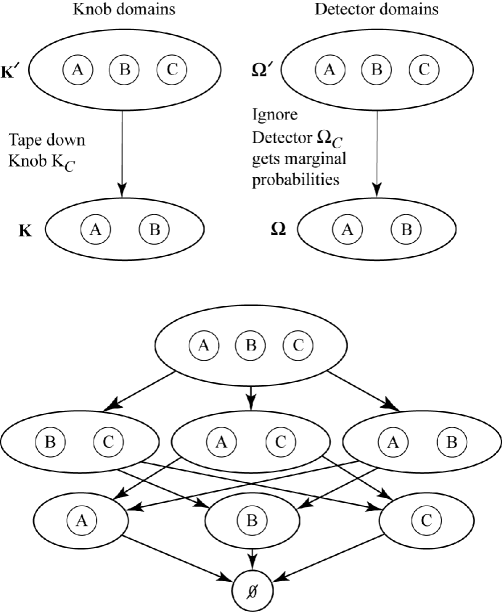
Figure 1: Lattices of domains.

A statement of (experimental) results, as expressed in quantum theory consists of the probability of outcome $\bm{j}\in\bm{\Omega}$ for each setting $\bm{k}$ of the knobs of $\bm{K}$, as illustrated in Fig. 2. We write $\mu(\bm{k},j)$ for this probability, and the probability function $\mu:\bm{K}\times\bm{\Omega}\rightarrow[0,1]$ is what we call a parametrized probability measure, that is, we have that for each $k_{A}\in K_{A}$, $k_{B}\in K_{B}$,  $\mu(k_{A},k_{B},-):\bm{\Omega}\rightarrow[0,1]$ is a probability measure on the set of detector outcomes. The quantum-mechanical form of experimental reports is that of a parametrized probability measure.

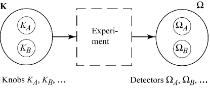
Figure 2: Quantum theory states experimental results as a parametrized probability measure $\mu:\ \mathbf{K}\to\mathrm{PrMeas}(\bm{\Omega})$.

For a given knob domain $\bm{K}$ and detector domain $\bm{\Omega}$, let PPM$(\bm{K},\bm{\Omega})$ be the space of all parametrized probability measures. When the number of knob settings and detections is finite, so is the dimension of this space. As illustrated in Sect. III for toy descriptions with finite numbers of knob settings and possible outcomes, parametrized probability measures constitute points of a function space that will play the part of a photograph onto which a larger space is mapped. Any $\mu\in\mbox{PPM}(\bm{K},\Omega)$ corresponds to a point on a photographic plate.

II.1 Explanations

A statement of results $\mu\!:\!\bm{K}\times\bm{\Omega}\rightarrow[0,1]$ says nothing about how its probabilities come about; that is the job of the explanatory part of a quantum description. An explanation of a statement of results consists of linear operators on some Hilbert space $\mathcal{H}$ as functions of the knob settings, including detection operators involving $\bm{\Omega}$. Products, tensor products, sums, exponentiations, etc. of operators are combined to form a triple $(\mathcal{H},\rho,M)$ in which $\rho$ and $M$ are functions on $\bm{K}$. The function $\rho\!:\!\bm{K}\rightarrow\{\mbox{density operators on }\mathcal{H}\}$ can be called a parametrized density operator, and the function $M\!:\!\bm{K}\times\bm{\Omega}\rightarrow\{\mbox{Detection operators on }\mathcal{H}\}$ is a parametrized positive operator-valued measure (POVM); more precisely, for each $\bm{k}\in\bm{K}$, it is the case that $M(\bm{k},-)\!:\!\bm{\Omega}\rightarrow\{\mbox{Detection operators on }\mathcal{H}\}$ is a POVM on $\bm{\Omega}$. The situation for continuous outcome spaces calls for the technicalities of measurable subsets, noted elsewhere tyler .

The explanations over a given knob domain $\bm{K}$ and detector domain $\bm{\Omega}$ consist in the set

$$\mbox{Expl}(\bm{K},\bm{\Omega})\buildrel\rm def\over{=}\{(\mathcal{H},\rho,M)\}$$ (1)

ranging over all $\mathcal{H}$, $\rho$ and $M$ of the form just stated. It is this space of explanations that turns out to be larger than the space of statements of results.

So defined, any explanation implies a statement of results via the familiar trace rule

$$(\forall\bm{k}\in\bm{K},\bm{\omega}\in\bm{\Omega})\quad\mu(\bm{k},\bm{\omega})=\mbox{Tr}_{\mathcal{H}}[\rho(\bm{k})M(\bm{k},\bm{\omega})],$$ (2)

where $\bm{\omega}\in\bm{\Omega}$ is an outcome. Often we abbreviate this by

$$\mu=\mbox{Tr}_{\mathcal{H}}(\rho M).$$ (3)

As we shall see, explanations, like “the stars in the sky,” are space of high dimension. The counting of degrees of freedom for explanations is a little involved, because we want to distinguish explanations that have conflicting natural extensions to larger knob domains. For this we introduce a notion of metric deviation, to which we now turn.

II.2 Metric deviation

Some differences among quantum explanations “make no difference.” For example if one explanation can be transformed into the other by the same unitary transformation applied both to the density operator and the POVM, the two explanations can be called “unitarily equivalent.” We are interested in descriptions that imply the same probabilities but that have more or less “natural” extensions to larger domains of knobs that, over the extended domain, conflict in their implied probabilities. For this it turns out to be handy to have a notion of metric deviation, which to our knowledge is a novelty. Before defining it, we start by recalling some operator metrics.

For density operators on a common Hilbert space $\mathcal{H}$, we use the metric defined by

$$\mbox{distance}[\rho(\bm{k}_{1}),\rho(\bm{k}_{2})]=\textstyle{\frac{1}{2}}\mbox{Tr}_{\mathcal{H}}|\rho(\bm{k}_{1})-\rho(\bm{k}_{2})|,$$ (4)

where for any bounded operator $A$, $|A|\buildrel\rm def\over{=}\sqrt{A^{\dagger}A}$. We choose this metric for density operators because it determines the least probability of error for deciding between two density operators on the basis of probabilities of outcomes helstrom .

While the trace metric and other operator metrics work only for operators on a common Hilbert space, another measure allows comparison of two parametrized density operators defined on different Hilbert spaces. Given $\rho\!:\!\bm{K}\rightarrow\mbox{DensOp}(\mathcal{H})$ and $\rho^{\prime}\!:\!\bm{K}\rightarrow\mbox{DensOp}(\mathcal{H}^{\prime})$, allowing that $\mathcal{H}^{\prime}$ can differ (even in dimension) from $\mathcal{H}$, we define the metric deviation of $\rho$ and $\rho^{\prime}$ by

$$\mbox{MetDev}(\rho,\rho^{\prime})\buildrel\rm def\over{=}\sup_{\bm{k}_{1},\bm{k}_{2}\in\bm{K}}\textstyle{\frac{1}{2}}\bm{|}\mbox{Tr}_{\mathcal{H}}|\rho(\bm{k}_{1})-\rho(\bm{k}_{2})|-\mbox{Tr}_{\mathcal{H}^{\prime}}|\rho^{\prime}(\bm{k}_{1})-\rho^{\prime}(\bm{k}_{2})|\bm{|}.$$ (5)

In case $\mbox{MetDev}(\rho,\rho^{\prime})=0$, we call $\rho$ and $\rho^{\prime}$ metrically equivalent; otherwise $\rho$ and $\rho^{\prime}$ are metrically inequivalent.

Remark: More familiar than metric equivalence is the notion of unitary equivalence, e.g. in the sense that $\rho$ and $\rho^{\prime}$ are unitarily equivalent if and only if there exists a unitary operator $U$ independent of $\bm{k}$ such that $(\forall\bm{k}\in\bm{K})\ \rho^{\prime}(\bm{k})=U\rho(\bm{k})U^{\dagger}$. Unitary equivalence implies metric equivalence, but not the converse: two parametrized density operators can be metrically equivalent without being unitarily equivalent. Example: $\rho(\bm{k})=\mbox{diag}(1/2-a_{k},1/2+a_{k}),\ 0<a_{k}<1$; then there exists $\delta>0$ such that $\rho^{\prime}(\bm{k})$ is same form with $a^{\prime}_{k}=a_{k}+\delta$. The $\delta$ cancels out of $\rho(\bm{k})-\rho(\bm{k}^{\prime})=\rho^{\prime}(\bm{k})-\rho^{\prime}(\bm{k}^{\prime})$, so the trace distance is invariant under the addition of $\delta$, demonstrating metric equivalence without unitary equivalence. (This addition of $\delta$ to $a_{k}$ is not a unitary transformation because it changes the eigenvalues.) Addition of an increment works also, and independently, for off-diagonal elements of generic density operators, where by generic we mean to rule out the special case of a unit eigenvalue or a zero eigenvalue.

Now turn to POVMs. Lifting the usual norm for bounded operators on a Hilbert space $\mathcal{H}$ to parametrized bounded operators gives a distance measure for parametrized POVMs over $\bm{K}\times\bm{\Omega}$

$$\mbox{distance}[M(\bm{k}_{1},-),M(\bm{k}_{2},-)]\buildrel\rm def\over{=}\sup_{\bm{\omega}\subset\bm{\Omega}}\|M(\bm{k}_{1},\bm{\omega})-M(\bm{k}_{2},\bm{\omega})\|_{\mathcal{H}}.$$ (6)

For two POVMs $M$ and $M^{\prime}$ (which can differ in both their Hilbert spaces $\mathcal{H}$ and $\mathcal{H}^{\prime}$, respectively and in their outcome domains $\bm{\Omega}$ and $\bm{\Omega}^{\prime}$) we define

$$\mbox{MetDev}(M,M^{\prime})\buildrel\rm def\over{=}\sup_{\bm{k}_{1},\bm{k}_{2}\in\bm{K}}\left|\sup_{\bm{\omega}\subset\bm{\Omega}}\|M(\bm{k}_{1},\bm{\omega})-M(\bm{k}_{2},\bm{\omega})\|_{\mathcal{H}}-\sup_{\bm{\omega}^{\prime}\subset\bm{\Omega}^{\prime}}\|M^{\prime}(\bm{k}_{1},\bm{\omega}^{\prime})-M^{\prime}(\bm{k}_{2},\bm{\omega}^{\prime})\|_{\mathcal{H}^{\prime}}\right|.$$ (7)

III Dimension counting for explanations and results

To pursue the analogy of “stars to photographs” we consider toy descriptions for which some interesting dimensions are finite. Let $\#\bm{K}$ be the number of settings of a knob domain $\bm{K}$, and let $\#\bm{\Omega}$ be the number of elementary outcomes for a detector domain $\bm{\Omega}$. (For a detector domain $\bm{\Omega}$ constituted of $n$ binary detectors, we have $\#\bm{\Omega}=2^{n}$.) Let $n_{\mathcal{H}}$ be the complex dimension of a finite-dimensional Hilbert space $\mathcal{H}$, so that a vector in $\mathcal{H}$ has $n_{\mathcal{H}}$ complex-valued components. Then the explanations $\{(\mathcal{H},\rho,M)\}$ involving the Hilbert space $\mathcal{H}$ form (at least locally) a real manifold of

$$\dim[\mbox{Expl}(\bm{K},\bm{\Omega})|_{\mathcal{H}}] \mskip-6.0mu=\mskip-6.0mu \#\bm{K}[n_{\mathcal{H}}^{2}(\#\Omega-1)+n^{2}_{\mathcal{H}}-1]=\#\bm{K}(n_{\mathcal{H}}^{2}\,\#\bm{\Omega}-1).$$ (8)

In contrast, the dimension of statements of results (“photographic plate”) is

$$\dim[\mbox{PPM}(\bm{K},\bm{\Omega})]=\#\bm{K}(\#\bm{\Omega}-1).$$ (9)

Subtracting the latter from the former, we find the space of explanations on $\mathcal{H}$ of a given statement of results has

$$\dim[\mbox{Tr}_{\mathcal{H}}^{-1}(\mu)] \mskip-6.0mu=\mskip-6.0mu \dim[\mbox{Expl}(\bm{K},\bm{\Omega})|_{\mathcal{H}}]-\dim[\mbox{PPM}(\bm{K},\bm{\Omega})]$$ (10)

$$\mskip-6.0mu=\mskip-6.0mu \#\bm{K}[n_{\mathcal{H}}^{2}(\#\bm{\Omega}-1)+n^{2}_{\mathcal{H}}-1]-\#\bm{K}(\#\bm{\Omega}-1)$$

$$\mskip-6.0mu=\mskip-6.0mu \#\bm{K}\,\#\bm{\Omega}(n_{\mathcal{H}}^{2}-1).$$

Thus there are lots of explanations of any given parametrized probability measure. The next point is that among these are metrically inequivalent explanations, as follows. For this paragraph, by class we mean an equivalence class on $\mbox{Tr}_{\mathcal{H}}^{-1}(\mu)$ defined by

$$(\mathcal{H},\rho,M)\equiv(\mathcal{H},\rho^{\prime},M^{\prime})\;\Leftrightarrow\;\mbox{MetDev}(\rho,\rho^{\prime})=\mbox{MetDev}(M,M^{\prime})=0.$$ (11)

By quotient space we mean the quotient space of $\mbox{Tr}_{\mathcal{H}}^{-1}(\mu)$ by this equivalence relation. The dimension of this quotient space is equal to the number of independent constraints imposed by the metric equivalence. For each pair of values $(\bm{k}_{1},\bm{k}_{2})$, the demand for metric equivalence places one constraint on parametrized density operators. For each pair of values of $(\bm{k}_{1},\bm{k}_{2})$ and each of the $\#\bm{\Omega}-1$ independent elements of the detector domain, the demand for metric equivalence places one constraint on detection operators. Altogether the number of constraints, independent or not, is given by

$$\#(\mbox{constraints})=\#\bm{K}(\#\bm{K}-1)\#\Omega/2,$$ (12)

from which we conclude that

$$\dim(\mbox{quotient space}) \mskip-6.0mu=\mskip-6.0mu \min(\#(\mbox{constraints}),\dim[\mbox{Tr}_{\mathcal{H}}^{-1}(\mu)])$$ (13)

$$\mskip-6.0mu=\mskip-6.0mu \min[\#\bm{K}(\#\bm{K}-1)\#\Omega/2,\#\bm{K}\,\#\bm{\Omega}(n_{\mathcal{H}}^{2}-1)].$$

Distinct points of this quotient space correspond to mutually metrically inequivalent explanations of a given parametrized probability measure, and we have just shown that there is an infinite set of mutually metrically inequivalent explanations. While we have shown this explicitly only for toy cases of finite numbers of knob settings and outcomes, the set of metrically inequivalent explanations of a given parametrized probability measure only gets larger when continuous sets of knob settings and outcomes are considered aop05 .

IV Avenues to explore

As Sam Lomonaco remarked, the showing of “multiple explanations” is analogous to the elementary proposition that through any countable set of points runs an infinitude of curves. From that point of view, what we have found is in a sense no surprise. Yet to accept that we live in a world of multiple, inequivalent explanations is to enter a new world, ready for exploration. Below are four examples.

IV.1 Results without explanations imply topologies on knob domains

Given that results can narrow possible explanations only to an infinite set, we wondered what results alone, without any choice of explanation, implied for the physics of knobs. One thing that results in the form of a parametrized probability measure imply is a topology on the knob domain. That is, starting with a knob domain $\bm{K}$ as a set without assuming a topology on it, any statement of results $\mu\!:\!\bm{K}\rightarrow\mbox{PrMeas}(\bm{\Omega})$ implies a topology $\tau_{\mu}$ on $\bm{K}$ that makes no assumption of any explanation:

$$\tau_{\mu}=\{U\subset\bm{K}|(\exists V\mbox{ open in PrMeas}(\bm{\Omega}))\quad U=\mu^{-1}(V)\},$$ (14)

(where $\mu^{-1}(V)=\{\bm{k}\in\bm{K}|\mu(\bm{k},-)\in V\}$). If $\mu$ is an injection into $\mbox{PrMeas}(\bm{\Omega})$, then the (bounded) uniform metric on $\mbox{PrMeas}(\bm{\Omega})$ induces a bounded metric on $\bm{K}$ tyler . If it is not injective, then $\mu$ induces a bounded metric on the quotient set of equivalence classes $\bm{K}/E_{\mu}$ where $E_{\mu}$ is the equivalence relation defined by

$$\bm{k}_{1}E_{\mu}\bm{k}_{2}\Leftrightarrow\mu(\bm{k}_{1},-)=\mu(\bm{k}_{2},-).$$ (15)

This metric, which we denote by $d_{\mu}$, is defined by

$$d_{\mu}([\bm{k}_{1}],[\bm{k}_{2}])\buildrel\rm def\over{=}\sup_{\bm{\omega}\subset\bm{\Omega}}|\mu(\bm{k}_{1},-)-\mu(\bm{k}_{2},-)|.$$ (16)

For $\mu\in\mbox{PPM}(\bm{K},\bm{\Omega})$ and $\mu^{\prime}\in\mbox{PPM}(\bm{K},\bm{\Omega}^{\prime})$ we add to our catalog of metric deviations by defining

$$\mbox{MetDev}(\mu,\mu^{\prime})\buildrel\rm def\over{=}\sup_{\bm{k}_{1},\bm{k}_{2}\in\bm{K}}\bm{\left|}|\mu(\bm{k}_{1},-)-\mu(\bm{k}_{2},-)|-|\mu^{\prime}(\bm{k}_{1},-)-\mu^{\prime}(\bm{k}_{2},-)|\bm{}.$$ (17)

If their metric deviation is zero, then $\mu$ and $\mu^{\prime}$ induce the same topological and metric structures on $\bm{K}$ tyler :

$$\mbox{MetDev}(\mu,\mu^{\prime})=0\Rightarrow E_{\mu}=E_{\mu^{\prime}},\;\tau_{\mu}=\tau_{\mu^{\prime}},\mbox{ and }\,d_{\mu}=d_{\mu^{\prime}}.$$ (18)

Examples of equivalence classes of knobs relevant to entangled states that violate Bell inequalities are discussed elsewhere ppm07 . When $\mu$ is not injective, the coarse topology $\tau_{\mu}$ on $\bm{K}$ induced by $\mu$ can be replaced by a finer topology by recognizing a finer level of description that augments the detector domain by adding another detector, as discussed below in connection with equivalence classes that characterize invariance.

IV.2 Endless cycle of extensions of inequivalent descriptions

Although the ambiguity of “Tr^-1” precludes results from logically forcing any single explanation, the existence of this ambiguity logically does force something, namely a dynamic that continually extends statements of results and explanations. From the proofs in Ref. aop05 and the lattice structure of knob domains and detector domains follows an endless open cycle of stating experimental results and explaining these results, illustrated in Fig. 3. This cycle operates in a context not limited to theory but including the experimental endeavors that theory describes. Although in this writing we cannot reach beyond quantum formalism to touch them, we have experiments in mind as a background against which a statement of results implied by an explanation can be judged and, if incompatible, rejected.

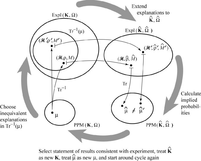
Figure 3: Expanding cycle of results and explanations.

Picture a “penguin” toy walking down a slope with a rolling gait, leaning left and swinging its right leg, then leaning right and swinging its left leg, on and on in a cycle. The swing of the left leg corresponds to choosing a pair of inequivalent explanations (which are guaranteed to exist as outlined in Sect. III). The swing of the right leg corresponds to calculating the parametrized probability measures implied by the natural extension of these explanations to a bigger knob domain, resulting in conflicting predicted probabilities. Experiments can eliminate at least one such probability measure extended over the bigger domain, but then the bigger knob domain serves as a base from which to “swing the left leg” and the cycle goes on, without end.

The details of the cycle for metrically inequivalent parametrized density operators are described elsewhere tyler . To show how the expanding cycle works when the metrically inequivalent elements of an explanation are the POVMs, we need the following.

Lemma: For $M$ and $M^{\prime}$ POVMs on a common knob domain $\bm{K}$ (but possibly involving distinct detector domains and distinct Hilbert spaces $\mathcal{H}$ and $\mathcal{H}^{\prime}$, respectively, MetDev$(M,M^{\prime})\neq 0$ implies that

$$(\exists\bm{k}_{1},\bm{k}_{2}\in\bm{K})\ \sup_{\sigma\in\mbox{DensOp}(\mathcal{H})}|\mbox{Tr}_{\mathcal{H}}\{\sigma[M(\bm{k},1)-M(\bm{k},1)]\}|$$ (19)

$$\mskip-6.0mu\neq\mskip-6.0mu \sup_{\sigma^{\prime}\in\mbox{DensOp}(\mathcal{H^{\prime}})}|\mbox{Tr}_{\mathcal{H}^{\prime}}\{\sigma^{\prime}[M^{\prime}(\bm{k},1)-M^{\prime}(\bm{k},1)]\}|.$$

Proof: Given any bounded hermitian operator $A$ on a Hilbert space $\mathcal{H}$, we have $\|A\|=\sup_{\|\mbox{$|x\rangle$}\|\leq 1}|\mbox{$\langle x|$}A\mbox{$|x\rangle$}|$; that is, the norm of a bounded hermitian operator equals its numerical radius bhatia . It is easy to show that the numerical radius is equal to $\sup_{\sigma\in\mbox{DensOp}(\mathcal{H})}\mbox{Tr}_{\mathcal{H}}(\sigma A)$. Thus we have the following proposition:

$$\|M(\bm{k}_{1},\bm{\omega})-M(\bm{k}_{2},\bm{\omega})\|=\sup_{\sigma\in\mbox{DensOp}(\mathcal{H})}|\mbox{Tr}_{\mathcal{H}}\{\sigma[M(\bm{k}_{1},\bm{\omega})-M(\bm{k}_{2},\bm{\omega})]\}|.$$ (20)

From this the proof of the lemma follows. Q.E.D.

Now we put the lemma to work. A way to distinguish the POVM $M(\bm{k}_{1},-)$ from $M(\bm{k}_{2},-)$ is to find the density operator $\sigma$ that maximizes the separation of the probability measures ensuing from these POVMs. Because of the lemma, when MetDev$(M,M^{\prime})\neq 0$, the separation of probabilities ensuing from the parametrized POVM $M$ differs from the separation of probabilities ensuing from $M^{\prime}$. Then if the explanations involving $M$ and $M^{\prime}$ are extended to a larger knob domain $\bm{K}^{\prime}$ that provides for $\sigma$ and $\sigma^{\prime}$, respectively, there results a conflict in the results implied by these extended explanations. Once that happens, one rejects at least one of the explanations, say on the basis of experiment, and keeps the other. Then one treats the extended knob domain $\bm{K}^{\prime}$ as a new starting knob domain, and off we go for another round of the cycle, as illustrated in Fig. 3. A take-home lesson is that a quantum description makes sense only as an element of a family of related descriptions, and the related descriptions spread out of larger and larger domains of knobs and detectors.

IV.3 The concept of invariance demands ambiguity of description

Now consider the concept of the invariances of a parametrized probability measure under changes of knob settings.

Remark: For those who like to think about Lorentz invariance of electromagnetic theory, we note that in the quantum context, the electromagnetic fields belong to the “explanation” part of the story, and explanations need not be Lorentz invariant. Indeed, neither classically nor in quantum theory is the electromagnetic field a Lorentz scalar. It is not the field as an explanation but the probabilities of detection, that are supposed to be the same for two experiments, one conducted for example in the inertial frame of train station, the other in the inertial frame of a train in uniform motion relative to the train station. Here we focus not on explanations but on “statements of results” expressed as parametrized probability measures.

An invariance in a parametrized probability measure $\mu$ asserts a non-trivial equivalence class on its knob domain $\bm{K}$, an equivalence class $[\bm{k}]$ defined by

$$[\bm{k}]=\{\bm{k}^{\prime}|\mu(\bm{k}^{\prime},-)=\mu(\bm{k},-)\}.$$ (21)

An example is a violation of Bell inequalities by which entanglement is demonstrated ppm07 . In that example the probability of coincidence detection by two rotatable detectors, one turned through an angle $k_{A}$, the other through an angle $k_{B}$ is $\mu(k_{A},k_{B},(1,1))=\textstyle{\frac{1}{2}}\cos^{2}(k_{A}-k_{B})$. This and the other relevant probabilities depend on $k_{A}$ and $k_{B}$ only as their difference $k_{A}-k_{B}$, so that a change defined by adding the same amount of rotation to each of these knobs leaves $\mu$ invariant.

But here is a conceptual muddle. If changing the knob settings makes no difference to the results, on what basis can we judge that any change in knob settings has taken place? A related question was put by one of our mathematician colleagues: Why not just “mod out” the equivalence classes? But it won’t do for physics to “mod out” such an equivalence class; the physicist wants not to make it disappear but to appreciate it.

One way to appreciate changes of knobs that make no difference to the results is to recognize, side by side with the statement of results $\mu$, a second statement of results $\mu^{\prime}$ at a finer level of detail, in particular a detector domain augmented by extra detectors to register changes in $k_{A}$ and $k_{B}$ separately. Then $\mu$ is seen as obtained from $\mu^{\prime}$ by ignoring the “extra” detectors:

$$\mu^{\prime}(k_{A},k_{B},(1,1,\Omega_{\rm knob}))=\mu(k_{A},k_{B},(1,1)).$$ (22)

Here $\Omega_{\rm knob}$ is the “anything-goes” or “don’t care” outcome of the extra detectors that respond to $k_{A}$ and $k_{B}$ separately, so that $\mu$ is seen as a marginal probability measure derived from ignoring “knob-motion detectors” in a more detailed statement of results $\mu^{\prime}$ that breaks invariance to show that $k_{A}$ and $k_{B}$ moved even if their difference was held fixed.

A second way to make sense of invariance of results is to understand the invariant parametrized probability measure $\mu$ over $\bm{K}$ as derived from a second parametrized probability measure $\mu^{\prime}$ over a larger knob domain $\bm{K}^{\prime}$ that contains an extra knob. $\mu$ is then obtained from $\mu^{\prime}$ by fixing the extra knob at a special value.

For example, to demonstrate rotational invariance we might place a disk on a table and rotate it to show that “nothing detectable changes under rotation.” But to see this invariance, whether one is aware of it or not, one must manage incompatible frames of reference byers . Looked at one way “nothing happens when we rotate the disk; but to see that “nothing happens when we rotate the disk” one must see in the other frame, so to speak, that in fact “the disk rotates.” This suggests adding a knob that can move the center of rotation away from the center of the disk. When the disk is off center, one sees its rotation. As the center of the disk is moved closer to the center of rotation, one approaches invariance.

Something similar can be worked out for the preceding example involving quantum states that violate Bell inequalities. When this is done, the equivalence class of knob settings show up as singular values sing in the mapping $\mu^{\prime}$ from knobs to probability measures, leading to another avenue for exploration.

IV.4 Remarks on quantum key distribution

Designs for quantum key distribution crypt assert security against undetected eavesdropping, based on transmitting quantum states that overlap, with the result that deciding between them with neither error nor an inconclusive result is impossible. The most popular design, BB84 BB84 , invokes four states (which we write as density operators) $\rho(1),\ldots,\rho(4)$. The claim of security invokes propositions such as this: if $\frac{1}{2}\mbox{Tr}|\rho(1)-\rho(2)|\leq\frac{1}{\sqrt{2}}$ then, by a well known result of quantum decision theory the least possible probability of error to decide between them is:

$$P_{E} \mskip-6.0mu\geq\mskip-6.0mu \textstyle{\frac{1}{2}}(1-\textstyle{\frac{1}{2}}|\rho(1)-\rho(2)|)=\textstyle{\frac{1}{2}}\left(1-\sqrt{\textstyle{\frac{1}{2}}}\right)\approx 0.146.$$ (23)

But how is one to rely on an implemented key-distribution system built from lasers and optical fibers and so forth to act in accordance with this explanation? If a system of lasers and optical fibers and so forth “possessed” a single explanation in terms of quantum states, one could hope to test experimentally the trace distance between the pair of states. But no such luck. The trouble is that trace distance is a property not of probabilities per se, which are testable, but of some one among the many explanations of those probabilities. While the testable probabilities constrain the possible explanations, and hence constrain trace distances, this constraint on trace distance is “the wrong way around”—a lower bound instead of a sub-unity upper bound on which security claims depend.

Given any parametrized probability measure, proposition 2 in Ref. aop05 assures the existence of an explanation in terms of a parametrized density operator $\rho^{\prime}$ metrically inequivalent to $\rho$, such that, in conflict with Eq. (23), the trace distance becomes $\textstyle{\frac{1}{2}}|\rho^{\prime}(1)-\rho^{\prime}(2)|=1$, making the quantum states in this explanation distinguishable without error, so that the keys that they carry are totally insecure.

The big question in key distribution is this: how will the lasers and fibers and detectors that convey the key respond to attacks in which an unknown eavesdropper brings extra devices with their own knobs and detectors into contact with the key-distributing system? Attacks entail knob and/or detector domains extended beyond those tested, with the possibility that extended explanations metrically inequivalent to that used in the design, but consistent with available probabilities, both imply a lack of security theoretically and accord with actual eavesdropping.

Physically, one way for insecurity to arise is by an information leak through frequency side-band undescribed in the explanation on which system designers relied. A more likely security hole appears when lasers that are intended to radiate at the same light frequency actually radiate at slightly different frequencies, as described in Refs. ppm07 ; spie05 ; Frwk .

V Concluding remarks

As discussed in Sect. IV.2 and illustrated by Fig. 3, the roominess of the inverse trace forces an open cycle of expanding descriptions, encompassing both expansions of explanations and expansions of statements of results, along with expansions of their knob domains and their outcome domains. The discussion of invariance in Sect. 4.3 shows how understanding each description as an element of a family of competing descriptions resolves what otherwise is a conceptual obstacle. In the example of quantum key distribution of Sect. IV.4, we see how isolating a single description as if competing descriptions were irrelevant confuses the role of quantum theory in cryptography, with negative implications for the validity of claims of security. The world of multiple, competing descriptions in which quantum engineering navigates is cartooned in Fig. 4.

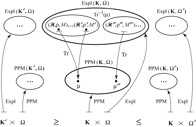
Figure 4: $\mathrm{Tr}^{-1}(\mu)$ contains many explanations.

References

- (1) P. A. M. Dirac, The Principles of Quantum Mechanics, 4th ed., Clarendon Press, Oxford, 1958.
- (2) J. von Neumann, Mathematische Grundlagen der Quantenmechanik, Springer, Berlin, 1932; translated with revisions by the author as Mathematical Foundations of Quantum Mechanics, Princeton University Press, Princeton, NJ, 1955.
- (3) J. M. Myers and F. Hadi Madjid, “Ambiguity in quantum-theoretical descriptions of experiments,” submitted to K. Mahdavi and D. Koslover, eds., AMS, Contemporary Mathematics series, Proceedings for the Conference on Representation Theory, Quantum Field Theory, Category Theory, Mathematical Physics and Quantum Information Theory, University of Texas at Tyler, 20–23 September 2007.
- (4) C. W. Helstrom, Quantum Detection and Estimation Theory, Academic Press, New York, 1976.
- (5) F. H. Madjid and J. M. Myers, “Matched detectors as definers of force,” Annals of Physics (NY) 319, pp. 251–273, 2005.
- (6) J. M. Myers and F. H. Madjid, “What probabilities tell about quantum systems, with application to entropy and entanglement,” in Philosophy of Quantum Information and Entanglement, A. Bokulich and G. Jaeger, eds., Cambridge University Press, in press.
- (7) R. Bhatia, Positive Definite Matrices, Princeton University Press, Princeton, NJ, 2007.
- (8) W. Byers, How Mathematicians Think: Using Ambiguity, Contradiction, and Paradox to Create Mathematics, Princeton University Press, Princeton, NJ, 2007.
- (9) V. I Arnold, S. M. Gusein-Zade, and A. N. Varchenko, Singularities of Differentiable Mappings, Vol. I, Birkhäuser, Boston, 1985.
- (10) N. Gisin, G. Ribordy, W. Tittel, and H. Zbinden, “Quantum cryptography,” Rev. Mod. Phys. 74, pp. 145–195, 2002.
- (11) C. H. Bennett and G. Brassard, “Quantum cryptography: Public key-distribution and coin tossing,” Proc. IEEE Int. Conf. on Computers, Systems and Signal Processing, Bangalore, India, pp. 175–179, IEEE, New York, 1984.
- (12) J. M. Myers, “Polarization-entangled light for quantum key distribution: how frequency spectrum and energy affect statistics,” Proceedings of SPIE, Vol. 5815, Quantum Information and Computation III, E. J. Donkor, A. R. Pirich, H. E. Brandt, eds., pp. 13–26, SPIE, Bellingham, WA, 2005.
- (13) J. M. Myers “Framework for quantum modeling of fiber-optical networks, Parts I and II,” quant-ph/0411107v2 and quant-ph/0411108v2, 2005.