The polarizability of the pion:
no conflict between dispersion theory and chiral perturbation theory

Abstract

Recent attempts to determine the pion polarizability by dispersion relations yield values that disagree with the predictions of chiral perturbation theory. These dispersion relations are based on specific forms for the absorptive part of the Compton amplitudes. The analytic properties of these forms are examined, and the strong enhancement of intermediate-meson contributions is shown to be connected with spurious singularities. If the basic requirements of dispersion relations are taken into account, the results of dispersion theory and effective field theory are not inconsistent.

I Introduction

The polarizabilities of a composite system such as the pion are elementary structure constants, just as its size and shape. They can be studied by applying electromagnetic fields to the system. The physical content of the polarizability can be visualized best by effective multipole interactions for the coupling of the electric $(\vec{E})$ and magnetic $(\vec{H})$ fields of a photon with the internal structure of the pion. This structure can be accessed experimentally by the Compton scattering process $\gamma+\pi\to\gamma+\pi$ or the crossed-channel reaction $\gamma+\gamma\to\pi+\pi$. When expanding the Compton scattering amplitude in the energy of the photon, the zeroth- and first-order terms follow from a low-energy theorem and can be expressed solely in terms of the charge and mass of the pion. The second-order terms in the photon energy describe the response of the pion’s internal structure to an external electric or magnetic dipole field, they are proportional to the electric ($\alpha)$ and magnetic ($\beta$) dipole polarizabilities, respectively. Expanding the Compton amplitudes to higher orders in the energy, one obtains higher-order polarizabilities, e.g., the quadrupole polarizabilities at fourth order.

From the theoretical side there is an extraordinary interest in a precise determination of the pion polarizabilities. Within the framework of the partially conserved axial-vector current (PCAC) hypothesis and current algebra the electromagnetic polarizabilities of the charged pion are related to the radiative decay $\pi^{+}\to e^{+}\nu_{e}\gamma$ Terentev:1972ix . The result obtained using chiral perturbation theory (ChPT) at leading non-trivial order (${\cal O}(p^{4})$) Bijnens:1987dc is equivalent to the original PCAC result, $\alpha_{\pi^{+}}=-\beta_{\pi^{+}}\sim\bar{l}_{\Delta}$, where $\bar{l}_{\Delta}\equiv(\bar{l}_{6}-\bar{l}_{5})$ is a linear combination of scale-independent parameters of the Gasser and Leutwyler Lagrangian Gasser:1983yg . At ${\cal O}(p^{4})$ this difference is related to the ratio $\gamma=F_{A}/F_{V}$ of the pion axial-vector form factor $F_{A}$ and the vector form factor $F_{V}$ of radiative pion beta decay Gasser:1983yg , $\gamma={\bar{l}}_{\Delta}/6$. Once this ratio is known, chiral symmetry makes an absolute prediction for the polarizabilities. Using the most recent determination $\gamma=0.443\pm 0.015$ by the PIBETA Collaboration Frlez:2003pe (assuming $F_{V}=0.0259$ obtained from the conserved vector current hypothesis) results in the ${\cal O}(p^{4})$ prediction $\alpha_{\pi^{+}}=2.64\pm 0.09$ in units of $10^{-4}\,\mbox{fm}^{3}$, where the estimate of the error is only the one due to the error of $\gamma$ and does not include effects from higher orders in the quark mass expansion.

Corrections to the leading-order PCAC result have been calculated at ${\cal O}(p^{6})$ in chiral perturbation theory and turn out to be rather small Burgi:1996qi ; Gasser:2006qa . Contrary to the situation of the nucleon, no “matter fields” with their own mass scale are present, and therefore the calculations can be performed in the original formulation of ChPT Gasser:1983yg . This makes the following predictions for the polarizabilities a very significant test of this theory Gasser:2006qa :

$$\alpha_{\pi^{+}}+\beta_{\pi^{+}} = 0.16\,,$$ (1)

$$\alpha_{\pi^{+}}-\beta_{\pi^{+}} = 5.7\pm 1.0\,.$$ (2)

The error for $\alpha_{\pi^{+}}+\beta_{\pi^{+}}$ is of the order 0.1, mostly from the dependence on the scale at which the ${\cal O}(p^{6})$ low-energy coupling constants are estimated by resonance saturation. The forward polarizability could also obtain relatively large contributions at ${\cal O}(p^{8})$. On the other hand, there is as yet no indication of large higher-order effects for the backward polarizability $\alpha_{\pi^{+}}-\beta_{\pi^{+}}$. For further information on low-energy $\pi\gamma$ reactions we refer to the recent review by Kaiser and Friedrich Kaiser:2008ss .

The pion polarizability has been studied in lattice QCD Wilcox:1996vx . The valence-quark contribution to the electric polarizability was shown to yield only the small value $\alpha_{\pi^{+}}\approx-0.17$, one order of magnitude smaller than the value predicted by ChPT. It is, of course, not surprising that sea quarks and their correlations must play an important role, most likely configurations with the quantum numbers of the pion. In a recent contribution, Hu et al. also conclude that polarizabilities are difficult to predict in lattice QCD because of (partial) quenching and volume effects Hu:2007ts . However, these authors point out that forthcoming lattice QCD results can be used as a diagnostic for ChPT.

The results of ChPT are in sharp contrast with the predictions of Fil’kov and Kashevarov Fil'kov:1982cx ; Fil'kov:1998np ; Fil'kov:2005ss ; Fil'kov:2005yf who obtain

$$11.1\leq\alpha_{\pi^{+}}-\beta_{\pi^{+}}\leq 15.6$$ (3)

in recent work Fil'kov:2005ss based on dispersion relations (DRs). The dispersion integrals are saturated by various meson contributions in the $s$ and $t$ channel. The free parameters are essentially fixed by the known masses, total widths, and partial decay widths of these mesons at resonance. However, the extrapolation to energies below and above the resonance is performed with specific resonance shapes whose analytic properties leave room for a considerable model dependence.

The very small value predicted by Eq. (1), that is Baldin’s sum rule applied to the pion, makes a measurement of this observable close to impossible. The experiments are therefore analyzed with the constraint $\alpha_{\pi^{+}}=-\beta_{\pi^{+}}$. Unfortunately, the experimental situation is rather contradictory, see Refs. Ahrens:2004mg ; Gasser:2006qa for recent reviews of the data and further references to the experiments. There exist basically three different methods to measure $\alpha_{\pi^{+}}$: (I) the reactions $e^{+}e^{-}\rightarrow\gamma\gamma\rightarrow\pi^{+}\pi^{-}$, (II) the Primakov effect of scattering a relativistic pion in the Coulomb field of a heavy nucleus, and (III) the radiative pion photoproduction, $p(\gamma,\gamma^{\prime}\pi^{+}n)$, which contains Compton scattering on an off-shell pion as a subprocess. The latter reaction was recently investigated at the Mainz Microtron MAMI with the result Ahrens:2004mg

$$\alpha_{\pi^{+}}-\beta_{\pi^{+}}=11.6\pm 1.5_{\text{stat}}\pm 3.0_{\text{syst}}\pm 0.5_{\text{mod}}\,,$$ (4)

which is at variance with the prediction of Gasser et al. Gasser:2006qa by two standard deviations. In view of the theoretical uncertainties from the fact that the photon is scattered by an off-shell pion, the deviation from theory is an open problem. In particular, we point out that the model error in Eq. (4) is estimated by comparing the analysis with 2 specific models. This does not exclude that a wider range of models will lead to larger model errors. Because the pion polarizability is extremely important for our understanding of QCD in the confinement region, it is prerequisite to check the given arguments by a full-fledged ChPT calculation of the reaction $p(\gamma,\gamma^{\prime}\pi^{+}n)$.

The second method to determine the polarizability, the Primakov effect, has been studied at Serpukhov with the result Antipov:1982kz

$$\alpha_{\pi^{+}}-\beta_{\pi^{+}}=13.6\pm 2.8_{\text{stat}}\pm 2.4_{\text{syst}}\,,$$ (5)

in agreement with the value from MAMI. Recently, also the COMPASS Collaboration at CERN has investigated this reaction, and the data analysis is underway Colantoni:2005ku ; Abbon:2007pq .

Unfortunately, the third method based on the reactions $e^{+}e^{-}\rightarrow\gamma\gamma\rightarrow\pi^{+}\pi^{-}$, has led to even more contradictory results in the range $4.4\leq\alpha_{\pi^{+}}\leq 52.6$, as listed in the work of Gasser et al. Gasser:2006qa . Therefore, one has to wait for an improved analysis of the data before final conclusions can be drawn. At the same time new and independent experimental effort is invaluable, such as the planned experiment at Jefferson Lab after the 12 GeV upgrade.

In this work we address the conflicting results obtained by ChPT and DRs. Section II gives a brief introduction to the kinematics and scattering amplitudes relevant for these studies. In Sec. III we summarize the elements of previous calculations in the framework of dispersion relations. Moreover, the approximations involved are critically investigated within several simple but pertinent approximations. Our results for dispersion relations in the $t$ channel are presented in Sec. IV. Finally, we give our conclusions in Sec. V.

II Kinematics and scattering amplitudes

Let us consider the kinematics of Compton scattering, the reaction $\gamma(k)+\pi(p)\rightarrow\gamma(k^{\prime})+\pi(p^{\prime})$, where the variables in brackets denote the 4-momenta of the participating particles. The familiar Mandelstam variables are

$$s=(k+p)^{2}\ ,\ \ t=(k-k^{\prime})^{2}\ ,\ \ u=(k-p^{\prime})^{2}\ ,$$ (6)

which are constrained by $s+t+u=2m^{2}$, where $m$ is the pion mass. The crossing-symmetric variable $\nu$ is defined by

$$\nu=\frac{s-u}{4m}\,.$$ (7)

The two Lorentz-invariant variables $\nu$ and $t$ span the Mandelstam plane shown in Fig. 1. They are related to the initial ($E_{\gamma}$) and final ($E^{\prime}_{\gamma}$) photon lab energies and to the lab scattering angle $\theta$ by

$$\nu = E_{\gamma}+\frac{t}{4m}=\frac{1}{2}(E_{\gamma}+E^{\prime}_{\gamma}),$$

$$t = -4E_{\gamma}\,E^{\prime}_{\gamma}\,\sin^{2}(\theta/2)=-2m(E_{\gamma}-E^{\prime}_{\gamma}).$$ (8)

The scattering matrix of Compton scattering on the pion, $T$, can be expressed by 2 independent amplitudes $A_{i}(\nu,t)$, $i=1,2$. These structure functions depend on $\nu$ and $t$, they are free of kinematic singularities and constraints, and because of the crossing symmetry they satisfy the relation $A_{i}(\nu,t)=A_{i}(-\nu,t)$. We further note that the functions $A_{i}$ are real in the interior of a triangle formed by the dashed lines $s=t=u=4m^{2}$ in Fig. 1. In the following we use these amplitudes to set up DRs. The amplitudes $A_{i}$ are related to the amplitudes $T_{i}$ of Prange Prange:1958dd as follows:

$$T_{1} = {\textstyle\frac{1}{2}}(tA_{1}+\eta A_{2})\,,$$

$$T_{2} = {\textstyle\frac{1}{2}}(tA_{1}-\eta A_{2})\,,$$ (9)

with $\eta=4\nu^{2}+t-t^{2}/(4m^{2})=(m^{4}-su)/m^{2}=((s-m^{2})^{2}+st)/m^{2}$. In terms of these amplitudes, the $T$ matrix takes the form

$$T=\frac{\varepsilon^{\prime}\cdot P^{\prime}\,\varepsilon\cdot P^{\prime}}{P^{\prime}\cdot P^{\prime}}T_{1}+\frac{\varepsilon^{\prime}\cdot N\,\varepsilon\cdot N}{N\cdot N}T_{2}\,,$$ (10)

where $\varepsilon$ and $\varepsilon^{\prime}$ are the photon polarization four-vectors in the initial and final states, respectively. Furthermore we have defined the following 4-vectors

$$K\; = {\textstyle\frac{1}{2}}(k^{\prime}+k)\,,\;P={\textstyle\frac{1}{2}}(p^{\prime}+p)\,,\;Q={\textstyle\frac{1}{2}}(k^{\prime}-k)\,,$$

$$P^{\prime} = P-\frac{P\cdot K}{K\cdot K}K\,,\quad N^{\mu}=\epsilon^{\mu\alpha\beta\gamma}P^{\prime}_{\alpha}Q_{\beta}K_{\gamma}\,,$$ (11)

with $\epsilon_{0123}=+1$. The differential cross section for Compton scattering is constructed from the $T$ matrix by

$$\left(\frac{d\sigma}{d\Omega}\right)_{\gamma\pi}=\Phi^{2}\left|T\right|^{2},\qquad\mbox{with}\qquad\Phi=\cases{\displaystyle\frac{1}{8\pi m}\frac{E^{\prime}_{\gamma}}{E_{\gamma}}&(lab frame)\cr\displaystyle\frac{1}{8\pi\sqrt{s}}&(c.m. frame),}$$ (12)

where

$$|T|^{2} = \frac{1}{4}\Big{(}t^{2}|A_{1}|^{2}+\eta^{2}|A_{2}|^{2}\Big{)}.$$ (13)

We further note that the $t$-channel reaction $\gamma\gamma\rightarrow\pi\pi$ is usually described by the amplitudes $M_{++}=-A_{1}/2$ and $M_{+-}=-A_{2}/(2m^{2})$, with indices referring to the polarization of the incident photons. These amplitudes describe the respective cross section as follows:

$$\left(\frac{d\sigma}{d\Omega}\right)_{\gamma\gamma} = \frac{1}{128\pi^{2}}\sqrt{\frac{t-4m^{2}}{t^{3}}}\bigg{\{}t^{2}\mid M_{++}\mid^{2}$$ (14)

$$+ \frac{1}{16}t^{2}(t-4m^{2})^{2}\sin^{4}{\theta^{\ast}}\mid M_{+-}\mid^{2}\bigg{\}}\,,$$

with $\theta^{\ast}$ the angle between the incident photon and the outgoing pion in the c.m. frame. The cross section for $\gamma+\gamma\rightarrow\pi^{0}+\pi^{0}$ is obtained by multiplying the r.h.s of Eq. (14) with a factor 1/2, which accounts for two identical particles in the final state.

Assuming analyticity and an appropriate high-energy behavior, the amplitudes $A_{i}$ fulfill unsubtracted DRs at fixed $t$,

$${\rm Re}A_{i}(\nu,t)\;=\;A_{i}^{B}(\nu,t)\;+\;{2\over\pi}\;{\mathcal{P}}\int_{\nu_{\mathrm{thr}}(t)}^{+\infty}d\nu^{\prime}\;\frac{\nu^{\prime}\;\mathrm{Im}_{s}A_{i}(\nu^{\prime},t)}{\nu^{\prime 2}-\nu^{2}}\;.$$ (15)

The Born terms $A_{i}^{B}$ describe photon scattering off a point-like pion, which leads to poles for $s=m^{2}$ and $u=m^{2}$ shown by the dash-dotted lines in Fig. 1. In terms of the orthogonal coordinates these pole lines are given by $\nu(t)=\pm\nu_{B}(t)=\pm t/4m$. Furthermore, $\mathrm{Im}_{s}A_{i}$ are the discontinuities across the $s$-channel cut of the Compton process and $\nu_{\text{thr}}(t)={\textstyle\frac{3}{2}m}+\nu_{B}(t)$ is the threshold for two-pion production in the $s$ channel. The sum of pole and contact terms takes the form

$$A_{1}^{B}(\nu,t)=A_{2}^{B}(\nu,t)=\frac{e^{2}\,q}{(\nu-\nu_{B})(\nu+\nu_{B})}\,,$$ (16)

where $q$ is 0 for neutral and 1 for charged pions. As is obvious from Eq. (16), the Born contributions to the invariant amplitudes have a pure pole structure. The $s$-channel cut starts at the lowest production threshold, which is given by intermediate two-pion states, i.e., $s_{\text{thr}}=4m^{2}$. The same cuts appear in the $t$ and $u$ channels (see Fig. 1). For DRs at constant $t\leq 0$, the crossing symmetry allows one to combine the $s$- and $u$-channel contributions in the form of Eq. (15).

Other types of DRs evade the $u$-channel contributions and replace them by the discontinuity in the $t$ channel. These are DRs at fixed $u=m^{2}$ or at constant angle, e.g., $\theta=180^{\circ}$. The former DRs take the form Fil'kov:1998np

$${\rm Re}A_{i}(s,t)\;=\;A_{i}^{B}(s,t)+\;\frac{1}{\pi}\;{\mathcal{P}}\bigg{\{}\int_{t_{\text{thr}}}^{+\infty}dt^{\prime}\;\frac{\mathrm{Im}_{t}A_{i}(t^{\prime},u=m^{2})}{t^{\prime}-t}+\int_{s_{\text{thr}}}^{+\infty}ds^{\prime}\;\frac{\mathrm{Im}_{s}A_{i}(s^{\prime},u=m^{2})}{s^{\prime}-s}\bigg{\}}\;,$$ (17)

with the constraint $s+t=m^{2}$. In particular, the polarizabilities are obtained at the point $s=m^{2}$ and $t=0$,

$$\alpha+\beta=-\frac{1}{4\pi m}\,A_{2}^{\text{disp}}(s=m^{2},\,t=0)\,,\quad\alpha-\beta=-\frac{1}{4\pi m}\,A_{1}^{\text{disp}}(s=m^{2},\,t=0),$$ (18)

with $A_{i}^{\text{disp}}$ the dispersive, i.e., non-pole contribution to the respective amplitude. For further convenience we introduce the dynamic polarizabilities

$$P^{(+)}(s,t)=-\frac{1}{4\pi m}\,A_{2}^{\text{disp}}(s,t)\,,\quad P^{(-)}(s,t)=-\frac{1}{4\pi m}\,A_{1}^{\text{disp}}(s,t)\,,$$ (19)

with $P^{(\pm)}(m^{2},0)=\alpha\pm\beta$.

In order to evaluate the dispersion integral in Eq. (15), the imaginary parts in the $s$ channel are determined by the unitarity relation, taking account of two-pion states and resonance contributions such as vector mesons in the intermediate state. The $t$-channel contribution of Eq. (17) is obtained in terms of unitarized partial-wave amplitudes following the method outlined in Refs. Drechsel:1999rf ; Drechsel:2002ar . In the $t$ channel, the amplitudes $A_{1}$ (or $M_{++}$) and $A_{2}$ (or $M_{+-}$) correspond to photon helicity differences of $\Lambda_{\gamma}=0$ and $\Lambda_{\gamma}=2$, respectively.

III Models

In this section we study 3 generic resonance models with the amplitudes

$$F_{A}(s) = \frac{1}{M^{2}-s-{\textstyle{\frac{1}{4}}}\Gamma_{0}^{2}-iM\Gamma_{0}}\,,$$ (20)

$$F_{B}(s) = \frac{1}{M^{2}-s-{\textstyle{\frac{1}{4}}}[\Gamma(s)]^{2}-iM\Gamma(s)}\,,$$ (21)

$$F_{C}(s) = \frac{1}{M^{2}-s-iM\Gamma(s)}$$ (22)

with

$$\Gamma(s)=\bigg{(}\frac{s-s_{0}}{M^{2}-s_{0}}\bigg{)}^{\frac{3}{2}}\;\Gamma_{0}.$$ (23)

The amplitude $F_{A}$ describes an ideal resonance, a fixed pole at $s=(M-{\textstyle{\frac{i}{2}}}\;\Gamma_{0})^{2}$. The amplitudes $F_{B}$ and $F_{C}$ have an energy-dependent width leading to a branch cut in $s$ from $s_{0}=4m^{2}$ to $+\infty$. The onset of the cut is given by the threshold for two-pion production, and the energy dependence of the width in Eq. (23) corresponds to a $P$-wave resonance, i.e., intermediate vector mesons like $\rho$ or $\omega$. For a general angular momentum $L$, the width opens like $(s-s_{0})^{(2L+1)/2}$. The amplitude $F_{C}$ is obtained in the small-width approximation, $\Gamma_{0}\ll M$, this form is used in the work of Fil’kov and Kashevarov Fil'kov:2005ss ; Fil'kov:2005yf . Furthermore, these authors introduce an energy-dependent coupling constant for the excitation and the decay of the intermediate vector meson,

$$g^{2}(s)=6\pi\sqrt{\frac{M^{2}}{s}}\bigg{(}\frac{M}{M^{2}-m^{2}}\bigg{)}^{3}\,\Gamma_{\gamma\pi}\,,$$ (24)

where $\Gamma_{\gamma\pi}$ is the partial width for the decay of the vector meson to a pion-photon state. Combining the above equations with Eq. (19), we find the following expressions for the dynamic polarizabilities:

$$P^{(+)}_{N}(s)=\frac{2m}{\pi}\,g^{2}(s)\,F_{N}(s),\quad P^{(-)}_{N}(s)=-\frac{2s}{\pi m}\,g^{2}(s)\,F_{N}(s)=-\frac{s}{m^{2}}\,P^{(+)}_{N}(s)\,.$$ (25)

This defines the models $A$, $B$, and $C$ discussed in the following. Due to the square-root singularity at the origin, the coupling of Eq. (24) leads to an (unphysical) cut from $s=-\infty$ to $s=0$. For this reason we also introduce models with an energy-independent coupling fixed by the value at the resonance position, $g_{0}^{2}=g^{2}(M^{2})$. These models are denoted by $A0$, $B0$, and $C0$. If all the requirements to set up the DRs are fulfilled, the direct calculation of the polarizabilities from the real part of the Compton amplitude has to yield the same result as obtained from the DRs with the imaginary part as input. For a comparison with the physics, the numerical calculations are performed for $m=M_{\pi+}=0.140$ GeV, $M=M_{\rho}=0.770$ GeV, $\Gamma_{0}=\Gamma_{\rho}=0.151$ GeV, and $\Gamma_{\gamma\pi}=\Gamma_{\rho\gamma\pi}=0.068$ MeV.

III.1 Forward polarizability

Let us first address the DR for the forward polarizability, $P^{(+)}$, which is obtained from the dispersion integral Eq. (15) evaluated at $t=0$ (forward DR). The results for the $s$-channel contribution are listed in Table 1. If the $u$ channel is also included, the full polarizability is obtained by multiplication with a factor 2 (crossing symmetry). Because the amplitude $F_{A0}$ does not have a cut, the dispersion integral runs over the full real axis. In the table, the integrals have been divided into the contributions above and below the physical branch point $s=s_{0}$, labeled “right cut” and “left cut”, respectively. The (unphysical) contribution of model $A0$ below the production threshold is clearly rather small. A look at the table shows that the models yield quite similar contributions from the right cut. However, the models differ substantially in their analytic structure. In particular, they differ because of the following ingredients:

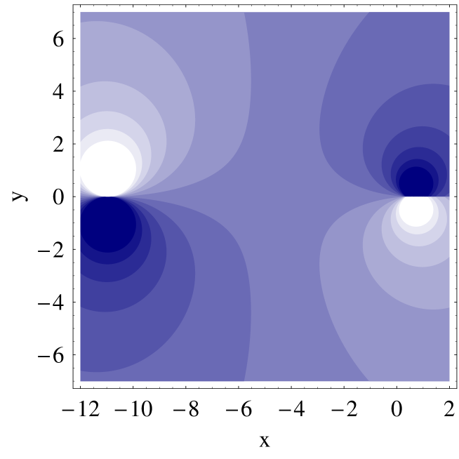
Figure 2: Contour plot of the imaginary part of the dynamical polarizability $P^{(+)}_{C0}$ in the complex $s=x+{\text{i}}\,y$ plane, with $x$ and $y$ in units of ${\text{GeV}}^{2}$. The cut due to two-pion intermediate states (right) leads from $x\approx 0.02$, $y=0$ to $x\rightarrow\infty$, $y=0$. The spurious pole of this model is seen on the left near $x=-11$.

• The energy-dependent width of models $B$, $B0$, $C$, and $C$0 introduces the correct physical cut starting at $s=4m^{2}$ and shifts the resonance pole to the second Riemann sheet. At the same time, this energy dependence leads to (unphysical) singularities of the amplitude on the first sheet: a pair of complex-conjugate poles in models $B0$ and $B$ as well as a (spurious) pole on the negative axis at $s\approx-11\leavevmode\nobreak\ {\text{GeV}}^{2}$ in model $C0$, that is, a deeply bound state of the pion-photon system. Independent of the physical questions involved with these models, we can not simply ignore these cuts and poles. As an example, Fig. 2 displays the imaginary part of the dynamic polarizability $P_{C0}^{(+)}$. Because the static polarizability is obtained at the small value $s=m^{2}$, close to the onset of the cut seen on the right side of the figure, the effect of the distant pole on the left is suppressed (see Table 1).

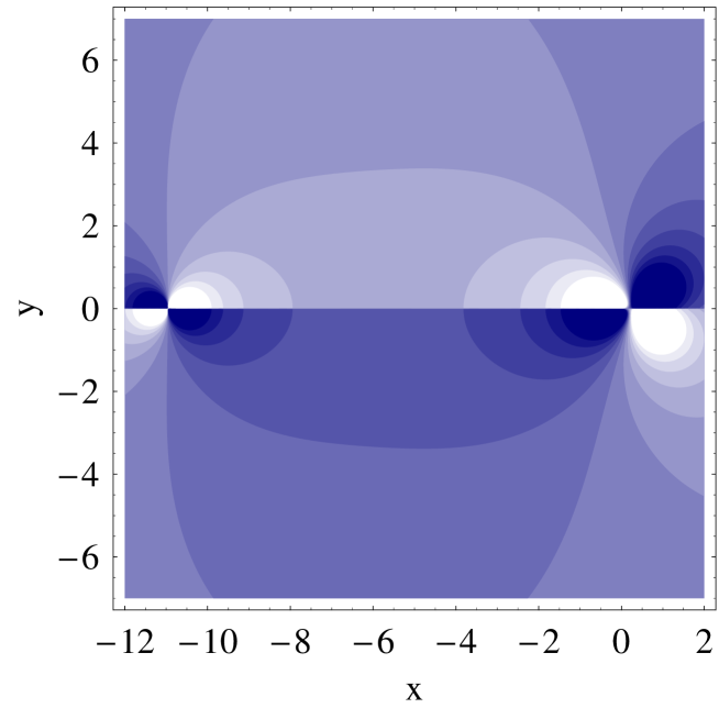
Figure 3: Contour plot of the imaginary part of the dynamical polarizability $P^{(+)}_{C}$ in the complex $s=x+{\text{i}}\,y$ plane, with $x$ and $y$ in units of ${\text{GeV}}^{2}$. The cut due to two-pion intermediate states (right) leads from $x\approx 0.02$, $y=0$ to $x\rightarrow\infty$, $y=0$. The (unphysical) left cut runs from $x=0$, $y=0$ to $x\rightarrow-\infty$, $y=0$. The spurious pole of Fig. 2 appears embedded on the left cut near $x=-11$.

• The energy-dependent coupling constant in models $A$, $B$, and $C$ leads to an even more serious problem, a $1/\sqrt{s}$ singularity at the origin resulting in a further cut. In order to obtain real values for the polarizabilities, we draw this cut from $s=0$ to $-\infty$ (left cut). Obviously, the square-root singularity is very close to the threshold of Compton scattering, $s=m^{2}$, in which point the polarizability is determined. Within the physical (right) cut, an energy dependence of the amplitudes with $1/\sqrt{s}$ may be a reasonable approximation, it increases the spectral function at energies below the resonance and damps the meson production at very large energies. However, the identification of the right-cut dispersion integral with the full amplitude at the Compton threshold is questionable, because the model introduces unphysical properties on the first sheet of the complex $s$ plane. In fact the left-cut contribution is dominant and leads to a considerable increase of the polarizabilities by a factor of $M/m$. As an example, the imaginary part of the dynamic polarizability $P_{C}^{(+)}$ is displayed in Fig. 3. The right cut in this figure has not changed much as compared to Fig. 2, whereas the additional left cut with the embedded pole structure at $s\approx-11\leavevmode\nobreak\ {\text{GeV}}^{2}$ has become the dominant feature. In particular, the onset of the spurious left cut at $s=0$ appears very close to the Compton threshold at $s=m^{2}$, and the consequences are seen in Tables 1 and 2.

In a somewhat different language, the polarizability $P(m^{2})$ can be represented by a contour integral along a small circle about $s=m^{2}$ with radius $\epsilon$,

$$P(m^{2})\;=\;\frac{1}{2\pi i}\oint\frac{P(s^{\prime})}{s^{\prime}-m^{2}}ds^{\prime}\,.$$ (26)

If we blow up the contour, we expect only contributions from the upper and lower rim of the cut from $s=s_{\text{thr}}$ to $+\infty$ and, possibly, from a full circle at infinity. Because the above amplitudes converge better than $1/s$ for large $s$, the contribution of the large circle converges to zero. Obviously, unphysical poles on the physical sheet and the unphysical left cut are obstacles for blowing up the contour, and therefore we have to add (I) the residues of the integrand $P(s^{\prime})/(s^{\prime}-s)$ at the poles and (II) the integral over the discontinuity of the imaginary part on the left cut in order to agree with the value given by the real part of the Compton amplitude. We hasten to add that all the above models have unphysical properties and therefore deserve further studies. However, it is our point to demonstrate that the experimentally known amplitude at resonance, $s=M^{2}$, can not be uniquely continued to the threshold for Compton scattering, $s=m^{2}$, but that such procedure leaves room for large model errors. It is also worth pointing out that in models $B$ and $C$ the crossing symmetry leads to four cuts, which cover the complete real axis with the result of complex (quasi-static) polarizabilities .

III.2 Backward polarizability

Let us now turn to the dispersion relation for the backward polarizability $P^{(-)}$. Compared to the forward polarizability $P^{(+)}$, the additional factor $s$ in Eq. (25) leads to a much slower convergence of the integrals. This is most evident for model $A0$. As shown in Table 2 the integral over the right cut is still finite but increased by a factor $M^{2}/m^{2}$ as compared to Table 1. However, this factor is canceled by the finite contribution of the circle at infinity. The latter contribution vanishes for all other models. Table 2 shows the increase of the right-cut integral by $M^{2}/m^{2}$ also by all the other models. The somewhat larger factor for $C0$ is due to the bad convergence in this model. However, also the contributions of the residues and the left cut have much increased, and as a result the full contour integral yields precisely the value predicted by the real part of the functions. Because of the additional factor $s$ with respect to the forward polarizability, a figure analogous to Fig. 2 is completely dominated by the spurious pole at $s\approx-11\leavevmode\nobreak\ {\text{GeV}}^{2}$ such that the effect of the $\rho$ meson is practically invisible. As a result the residue of the spurious pole cancels the contribution of the right cut nearly completely. In a similar way, the spurious left cut due to the $1/\sqrt{s}$ ansatz in model $F_{C}$ cancels 85 % of the contribution of the (physical) right cut. As required by Eq. (25), we find the relation $P^{(+)}(s=m^{2})=-P^{(-)}(s=m^{2})$ not only for the real parts of the model amplitudes but also by summing up all the contributions to the contour integral. In spite of relatively small differences among the models near the resonance region, the polarizabilities predicted by considering only the right cut differ by an order of magnitude. We conclude that the extrapolation from the resonance position to the threshold of Compton scattering is dangerous, in particular, if performed with functions containing unphysical singularities. Because the $\omega$ and $\sigma$ mesons are the most important agents in the dispersion analysis of Refs. Fil'kov:2005ss ; Fil'kov:2005yf , we have also studied these cases. The numerical calculations for the $\omega$ meson are performed for $M=M_{\omega}=0.782$ GeV, $m=M_{\pi^{0}}=0.135$ GeV, $\Gamma_{0}=\Gamma_{\omega}=8.41$ MeV, and $\Gamma_{\gamma\pi}=\Gamma_{\omega\gamma\pi}=0.715$ MeV. Except for its larger photon decay branch and the smaller width, the $\omega$ follows the above exercise for the $\rho$ very closely, see Tables 3 and 4. In particular we observe the same overestimation of $\alpha-\beta$ by the dispersion integral along the right cut in the $s$ channel.

The scalar $\sigma$ meson is the dominant agent for the $t$-channel reaction. In the following we describe this meson with the parameters of model (a) given by Table 1 of Ref. Fil'kov:1998np , in particular $M=M_{\sigma}=0.547$ GeV, $m=M_{\pi^{+}}=0.140$ GeV, $\Gamma_{0}=\Gamma_{\sigma}=1.204$ GeV, and $\Gamma_{\gamma\pi}=\Gamma_{\sigma\gamma\pi}=0.62$ keV. Our models $A0$, $B$, and $C0$ are defined as above, that is with an energy-independent coupling constant fixed at resonance and with propagators given by Eqs. (20) - (23). The models $A$, $B$, and $C$ contain an energy-dependent coupling constant and for models $B$ and $C$ an additional energy-dependence of the width involving ${\sqrt{t}}$ factors. In particular, model $C$ corresponds to the expressions found in the Appendix of Ref. Fil'kov:1998np . Because of the spin $J=0$ of the $\sigma$, the width opens like a square root at threshold. The low mass and the huge width of the $\sigma$ lead to quite different analytical structures as compared to the vector mesons. Whereas models $A$ and $A_{0}$ with their constant widths yield a pole at the complex mass $t=(M-i\,\Gamma_{0}/2)^{2}$, this pole has been moved onto the second sheet for $B$ and $B0$, and in the case of $C$ and $C0$ the $\sigma$ pole has completely disappeared. The assumed analytical form also leads to a reasonable convergence of the dispersion integral over the right cut. However, the ansatz of Ref. Fil'kov:1998np results in a left cut with a singularity at $t=0$ leading to a dispersion integral with an integrand like $t^{-3/2}$ near the origin. As a consequence the integral diverges like $t^{-1/2}$ for $t\rightarrow 0$, at which point the polarizability is defined. The numerical results are listed in Table 5.

IV Dispersion relations in the $t$ channel

The amplitudes $A_{1}$ and $A_{2}$ introduced in Sec. II correspond to photon helicity differences $\Lambda_{\gamma}=0$ and $\Lambda_{\gamma}=2$, respectively. They have the following partial-wave expansions involving total angular momentum $J\geq\Lambda_{\gamma}$ and even isospin $I=0,\,2$:

$$A_{1}^{I} = \sum_{J\geq 0}\sqrt{2J+1}{\cal A}_{J0}^{I}P_{J}^{0}(\cos\theta^{*}),$$

$$\quad A_{2}^{I} = \sum_{J\geq 2}\sqrt{2J+1}\sqrt{\frac{(J-2)!}{(J+2)!}}{\cal A}_{J2}^{I}\frac{P_{J}^{2}(\cos\theta^{*})}{(1-\cos^{2}\theta^{*})},$$ (27)

where $\theta^{*}$ is the scattering angle in the c.m. system. The isospin decomposition of the physical channels is given by

$$A_{i}(\gamma\gamma\rightarrow\pi^{+}\pi^{-})=\sqrt{\frac{1}{3}}A_{i}^{I=0}+\sqrt{\frac{1}{6}}A_{i}^{I=2},$$

$$A_{i}(\gamma\gamma\rightarrow\pi^{0}\pi^{0})=\sqrt{\frac{1}{3}}A_{i}^{I=0}-\sqrt{\frac{2}{3}}A_{i}^{I=2}.$$ (28)

The partial waves ${\cal A}_{J\Lambda_{\gamma}}^{I}$ correspond to eigenstates of the scattering matrix, and their imaginary parts can be constructed by unitarity as follows:

$${\rm Im}{\cal A}_{J\Lambda_{\gamma}}^{I}(\gamma\gamma\rightarrow\pi\pi)=\sum_{n}\rho_{n}{\cal A}_{J\Lambda_{\gamma}}^{I}(\gamma\gamma\rightarrow n){\cal I}_{J\Lambda_{\gamma}}^{I}(n\rightarrow\pi\pi),$$ (29)

with $\rho_{n}$ the density of states for each channel $n$ and ${\cal I}$ the hadronic amplitude for the decay $n\rightarrow\pi\pi$. In the elastic region, the sum on the right hand side of Eq. (29) is saturated by the two-pion channel and, as an immediate consequence, the phase $\phi^{I}_{J\Lambda_{\gamma}}$ of each partial wave equals the corresponding pion-pion phase shift $\delta^{I}_{J}\equiv{\rm arg}\,{\cal I}^{I}_{J}(\pi\pi\rightarrow\pi\pi)$. This fact can be incorporated into the Omnès function, which is constructed to have the phase of the $\pi\pi$ scattering amplitude above two-pion threshold and to be real otherwise,

$${\Omega^{I}_{J}}(t)\;=\;\exp{\left[\frac{t}{\pi}\;{\int_{4m^{2}}^{\infty}}\,dt^{\prime}\,\frac{{\delta^{IJ}_{\pi\pi}}(t^{\prime})}{t^{\prime}(t^{\prime}\,-\,t\,-\,i\varepsilon)}\right]}\;.$$ (30)

The function ${\cal A}^{I}_{J\Lambda_{\gamma}}(t)/\Omega^{I}_{J}(t)$ is by construction real above $\pi\pi$ threshold and has a left cut ${\cal H}^{I}_{J\Lambda_{\gamma}}(t)$ generated for $t<0$ by the Born term and for $t<-(M_{V}^{2}-m^{2})/M_{V}^{2}$ by the exchange of vector mesons like the $\rho$ and $\omega$ vector mesons in the $s$ and $u$ channels. Hence the difference $\left[{\cal A}_{J\Lambda_{\gamma}}^{I}(t)-{\cal H}^{I}_{J\Lambda_{\gamma}}(t)\right]/\Omega^{I}_{J}(t)$ has only a right cut from $t=4m^{2}$ to $\infty$, and satisfies the following dispersion relation:

$${\cal A}^{I}_{J\Lambda_{\gamma}}(t)\, = \,\Omega^{I}_{J}(t)\;\bigg{\{}{\cal H}^{I}_{J\Lambda_{\gamma}}(t)\,\mathrm{Re}\left[(\Omega^{I}_{J})^{-1}(t)\right]$$ (31)

$$- \frac{(t\,-\,4m^{2})^{(J-\Lambda_{\gamma})/2}}{\pi}\,\int^{\infty}_{4m^{2}}\,dt^{\prime}\,\frac{{\cal H}^{I}_{J\Lambda_{\gamma}}(t^{\prime})\,\mathrm{Im}\left[(\Omega^{I}_{J})^{-1}(t^{\prime})\right]}{(t^{\prime}\,-\,4m^{2})^{(J-\Lambda_{\gamma})/2}(t^{\prime}\,-\,t)}\bigg{\}}\,,$$

with the factor $(t^{\prime}-4m^{2})^{(J-\Lambda_{\gamma})/2}$ providing the right asymptotic behavior for the convergence of the integral. In particular, the S-wave amplitude is given by

$${\cal A}^{I}_{00}=\Omega^{I}_{0}(t)\,\bigg{\{}{\cal H}^{I}_{00}(t)\,\mathrm{Re}\left[(\Omega^{I}_{0})^{-1}(t)\right]-\frac{1}{\pi}\,\int^{\infty}_{4m^{2}}\,dt^{\prime}\,\frac{{\cal H}^{I}_{00}(t^{\prime})\,\mathrm{Im}\left[(\Omega^{I}_{0})^{-1}(t^{\prime})\right]}{(t^{\prime}\,-\,t)}\bigg{\}}.$$ (32)

Furthermore, we define the generalized Born term as

$$H_{i}=A_{i}^{B}+A^{V}_{i},$$ (33)

with $A_{i}^{B}$ the Born term of Eq. (16) and the vector-meson contributions $A^{V}_{i}$ given by Ref. Ko:1989yd

$$A^{V}_{1}(s,t) = -2e^{2}R_{V}\left[\frac{s}{s-M_{V}^{2}}+\frac{u}{u-M_{V}^{2}}\right],$$ (34)

$$A^{V}_{2}(s,t) = 2e^{2}m^{2}R_{V}\left[\frac{1}{s-M_{V}^{2}}+\frac{1}{u-M_{V}^{2}}\right],$$ (35)

where $R_{V}$ are determined from the condition Donoghue:1993kw

$$R_{V}=\frac{24\pi M^{3}_{V}}{e^{2}}\frac{\Gamma(V\rightarrow\pi\gamma)}{(M_{V}^{2}-m^{2})^{3}}\;.$$ (36)

The comparison with Eqs. (20) - (25) in the zero-width approximation yields the relation $e^{2}R_{V}=4g^{2}_{V}(M_{V}^{2})$, with $g_{V}^{2}(M_{V}^{2})$ the coupling of Eq. (24) at resonance. In the following we only discuss the most important vector mesons, the $\rho(770)$ and $\omega(782)$.

At energies $W_{\pi\pi}=\sqrt{t}<1\leavevmode\nobreak\ {\text{GeV}}$ the phases are only large for the partial waves with $I=J=0$, and therefore most of the final-state interaction is contained in $\Omega^{I}_{00}$. We construct these S waves with the phase shifts given by Ref. Froggat:1977dd . The S-wave projections of the Born and vector meson contributions read

$${\cal B}^{I=0}_{00} = \frac{1}{\sqrt{2}}{\cal B}^{I=2}_{00}=-2e^{2}\frac{2}{\sqrt{3}}\frac{1-\beta^{2}}{t\beta}{\rm ln}\left(\frac{1+\beta}{1-\beta}\right),$$ (37)

$${\cal V}^{I=0}_{\rho\,00} = 4e^{2}\sqrt{3}\frac{R_{\rho}}{t}\left[\frac{M_{\rho}^{2}}{\beta}{\rm ln}\left(\frac{1+\beta+t_{\rho}/t}{1-\beta+t_{\rho}/t}\right)-t\right],$$ (38)

$${\cal V}^{I=2}_{\rho\,00} = 0,$$ (39)

$${\cal V}^{I=0}_{\omega\,00} = -\frac{1}{\sqrt{2}}{\cal V}^{I=2}_{\omega\,00}=\frac{4e^{2}}{\sqrt{3}}\frac{R_{\omega}}{t}\left[\frac{M_{\omega}^{2}}{\beta}{\rm ln}\left(\frac{1+\beta+t_{\omega}/t}{1-\beta+t_{\omega}/t}\right)-t\right],$$ (40)

where $t_{V}=2(M^{2}_{V}-m^{2})$ and $\beta=\sqrt{1-4m^{2}/t}$.

Because the phases of the higher partial waves are generally small for $W_{\pi\pi}<1\leavevmode\nobreak\ {\text{GeV}}$, they can be well described by the generalized Born amplitude in this region, and their contribution to the polarizability can be neglected. However, the $\gamma\gamma\rightarrow\pi\pi$ process has a distinct resonance structure corresponding to the isoscalar $f_{2}(1270)$ resonance with mass $M_{f_{2}}=1275$ MeV and width $\Gamma_{f_{2}}=185$ MeV. This resonance shows up in the partial wave ${\cal A}_{22}^{0}$ and therefore contributes only to the amplitude $A_{2}^{0}$. We model this contribution according to Ref. Drechsel:1999rf by the Breit-Wigner ansatz

$$A_{2}^{f_{2}}\;=\;e^{2}\,\frac{m^{2}}{M_{f_{2}}^{2}}\,\frac{g_{f_{2}\gamma\gamma}\,g_{f_{2}\pi\pi}}{M_{f_{2}}^{2}\,-t\,-\,iM_{f_{2}}\,\Gamma_{0}}\;,$$ (41)

where the coupling constant $g_{f_{2}\pi\pi}$ is known from the decay $f_{2}\rightarrow\pi\pi$, $g_{f_{2}\pi\pi}=23.65$ Yao:2006px , and $g_{f_{2}\gamma\gamma}$ is fitted to the $\gamma\gamma\rightarrow\pi\pi$ cross section at the resonance position, resulting in $g_{f_{2}\gamma\gamma}\approx 0.247$ consistent with Ref. Yao:2006px . As a result the $f_{2}$ resonance contribution is $(\alpha+\beta)^{\pi^{0}}_{f_{2}}=(\alpha+\beta)^{\pi^{+}}_{f_{2}}=0.17$.

With the unitarized S-wave contribution from Eq. (32) and, for the higher partial waves, the generalized Born contribution of Eq. (33) and the $f_{2}$ resonance contribution of Eq. (41), the full $t$-channel amplitudes can be cast into the form

$$A^{I}_{1}(s,t)\, = {\cal A}^{I}_{00}-{\cal H}^{I}_{00}(t)+H^{I}_{1}(s,t),$$

$$A^{I}_{2}(s,t)\, = \,H^{I}_{2}(s,t)+A_{2}^{I\,f_{2}}(s,t).$$ (42)

These amplitudes lead to the following results for the polarizabilities:

$$\alpha-\beta = -\frac{1}{4\pi m}\left(A_{1}^{V}(m^{2},0)-\frac{1}{\pi}\int^{\infty}_{4m^{2}}\,dt^{\prime}\,\frac{{\cal H}^{I}_{00}(t^{\prime})\mathrm{Im}\left[(\Omega^{I}_{0})^{-1}(t^{\prime})\right]}{t^{\prime}}\right),$$ (43)

$$\alpha+\beta = -\frac{1}{4\pi m}(A_{2}^{V}(m^{2},0)+A_{2}^{f_{2}}(m^{2},0)).$$ (44)

Because Eqs. (34) and (35) yield $A_{1}^{V}(m^{2},0)=-A_{2}^{V}(m^{2},0)>0$, it follows from the above equations that the vector mesons contribute only to the magnetic polarizability $\beta$. This effect is paramagnetic because the quark spins are aligned in the transition $\pi\rightarrow V$. If we compare with the results of Sec. III, the vector-meson contributions in Eqs. (43) and (44) correspond to the $s$-channel term in the fixed-$u$ dispersion relation of Eq. (17), whereas the dispersion integral in Eq. (43) and the $f_{2}$ resonance contribution in Eq. (44) can be identified with the $t$-channel dispersive contribution in Eq. (17). Focussing on the $t$-channel term, Fig. 4 shows the difference of the polarizabilities $\alpha-\beta$ of Eq. (43) as a function of the upper limit of integration in the region $4m^{2}\leq t_{\text{upper}}\leq 0.78\leavevmode\nobreak\ {\text{GeV}}^{2}$. The latter value is defined by the onset of inelasticities in the $\pi\pi$ phase shifts. As shown by the figure, the $I=0$ channel (with the quantum numbers of the $\sigma$ meson) provides a contribution of only about 5 units to the backward polarizability, about half of the value predicted by Fil'kov:2005ss . The bottom panels show the results for the generalized Born term ${\cal H}^{I}_{00}={\cal B}^{I}_{00}+{\cal V}^{I}_{00}$, including the $\rho$ and $\omega$ contributions, whereas the top panels are obtained with only the Born term ${\cal B}^{I}_{00}$. Furthermore, Fig. 4 shows the results for both the $I=0$ channel only (dashed lines) and the sum of the $I=0$ and $I=2$ channels (solid lines).

The $\gamma\gamma\rightarrow\pi\pi$ cross section is obtained from the amplitudes of Eq. (42) with the S-wave contribution evaluated by the following subtracted DR:

$${\cal A}^{I}_{00}(t)\, = \,\Omega^{I}_{0}(t)\;\bigg{\{}{\cal H}^{I}_{00}(t)\,\mathrm{Re}\left[(\Omega^{I}_{0})^{-1}(t)\right]$$ (45)

$$+ c^{I}_{00}-\frac{t}{\pi}\,\int^{\infty}_{4m^{2}}\,dt^{\prime}\,\frac{{\cal H}^{I}_{00}(t^{\prime})\,\mathrm{Im}\left[(\Omega^{I}_{0})^{-1}(t^{\prime})\right]}{t^{\prime}(t^{\prime}\,-\,t)}\bigg{\}},$$

where the subtraction constants $c^{I}_{00}$ are related to the polarizabilities by

$$c^{I=0}_{00} = -8\pi m\frac{1}{\sqrt{3}}\left[(\alpha-\beta)^{\pi^{+}}+\frac{1}{2}(\alpha-\beta)^{\pi^{0}}\right]-A_{1}^{V,I=0}(m^{2},0),$$ (46)

$$c^{I=2}_{00} = -4\pi m\sqrt{\frac{2}{3}}\left[(\alpha-\beta)^{\pi^{+}}-(\alpha-\beta)^{\pi^{0}}\right]-A_{1}^{V,I=2}(m^{2},0).$$ (47)

Figure 5 displays the total $\gamma\gamma\rightarrow\pi^{+}\pi^{-}$ cross section given by the subtracted DRs of Eq. (45) with subtraction constants fixed by ChPT and the model of Ref. Fil'kov:2005yf as well as the results obtained from the unsubtracted DR for only the S-wave amplitude, see Eq. (32). We note that all the results are obtained with an energy-independent coupling constant $g_{V}(M_{V}^{2})$. The same results are shown over a larger energy region in Fig. 6. The $f_{2}$ resonance contribution is clearly visible near $W_{\pi\pi}=1.2$ GeV. However, the contribution of this resonance to the polarizability is very small, as has been noted before.

The corresponding results for the $\gamma\gamma\rightarrow\pi^{0}\pi^{0}$ cross section are shown in Fig. 7. For this reaction the differences among the models are much more pronounced, and at energies above the $f_{2}$ resonance the discussed method fails completely, most likely because of the inelasticities due to more-pion and heavier systems. In order to highlight the importance of the vector mesons, Fig. 8 presents the results of the previous figure without the vector-meson contributions. A correct unitarization of the full amplitude will be required in order to describe the higher-energy region. Such a more consistent treatment has been developed, for instance, in Refs. Kaloshin:1986yy and Kaloshin:1993wj . The large model dependency for the neutral pion channel has also been observed in the recent work of Oller and Roca Oller:2008kf . Finally, we present our predictions for $\alpha-\beta$ in Table 6, as obtained from unsubtracted DRs. The value for the charged pion is in excellent agreement with ChPT, whereas we fail to get close to the ChPT prediction for the neutral pion. In view of the previous figures, this result is not too surprising. Whereas our unitarized amplitude describes the $\pi^{+}$ cross section quite well up to energies of about 2 GeV (see the solid lines in Figs. 5 and 6), the corresponding results for the $\pi^{0}$ cross section are unsatisfactory (see the solid lines in Figs. 7 and 8). A comparison of the two latter figures shows the large dependence on the background from meson exchange. Furthermore, the results for the $\pi^{0}$ cross section from unsubtracted DRs do not describe the data for energies above 500 MeV. A much better description of the data is obtained by the subtracted DR with the subtraction constant as predicted by ChPT at the two-loop level Bellucci:1994eb (dashed line in Fig. 7).

V Conclusion

The polarizabilities of the pion are elementary structure constants and therefore fundamental benchmarks for our understanding of QCD in the confinement region. Moreover, these polarizabilities have been calculated in ChPT to the two-loop order with an estimated error of less than 20 %. It is therefore disturbing that predictions based on dispersion theory Fil'kov:2005ss yield $\alpha_{\pi^{+}}-\beta_{\pi^{+}}$ in the range of $11-15$, whereas ChPT Gasser:2006qa predicts $5.7\pm 1.0$, all in units of $10^{-4}\leavevmode\nobreak\ {\text{fm}}^{3}$. This discrepancy originates from huge contributions of intermediate meson states in the approach of Ref. Fil'kov:2005ss . In particular, the $\sigma$ exchange in the $t$ channel provides about 10 units for both neutral and charged pions. For neutral pions, this $\sigma$ contribution is canceled by vector mesons, notably $\omega$ exchange yielding a value of $-13$, with the result of $\alpha_{\pi^{0}}-\beta_{\pi^{0}}\approx-3$. The large positive value for charged pions results because (I) the $\omega$ does not contribute in this case and (II) axial vector mesons provide additional positive contributions of about 4 units. In ChPT, on the other hand, the vector mesons enter only at ${\cal{O}}(p^{6})$ through vector-meson saturation of low-energy constants. They are usually treated in the zero-width approximation and estimated to yield a much smaller effect for the polarizability, e.g., the $\omega$ contributes only about 1 unit to the neutral pion polarizability Donoghue:1993kw ; Bellucci:1994eb . The apparent discrepancy between the two approaches can be attributed to the specific forms for the imaginary part of the Compton amplitudes Fil'kov:2005ss ; Fil'kov:2005yf , which serve as input for the dispersion integrals determining the polarizability at the Compton threshold ($s=m^{2},\,t=0$). In order to quantify the strong model dependence of this procedure, we have studied six different analytical forms including the model of Refs. Fil'kov:2005ss ; Fil'kov:2005yf . We recall that all these models are fitted to the same masses and widths of the exchanged mesons, and in this sense they represent the experimentally known information in the same way. Concentrating on the important $\omega$ meson and the forward polarizability, we find from Table 3 that the models $A0$, $B0$, and $C0$ (with a constant coupling strength) predict a contribution of about 0.7 for the sum of $s$ and $u$ channel, in reasonable agreement with Ref. Donoghue:1993kw ; Bellucci:1994eb . The energy dependence of the coupling constant in models $A$, $B$, and $C$ leads to an unphysical left cut (see Fig. 3) and increases the contribution to the real part by a factor $M_{\omega}/m\approx 7$. However, all the models agree if only the right cut is accounted for. If we now turn to the backward polarizability, we expect from Eq. (25) that the paramagnetic dipole transition involved leads to a mere sign change compared to the forward polarizability, as is indeed reproduced by the real part in Table 4. However, the right-cut integral has increased to large absolute values. As a consequence, the dispersion integral over the right cut from two-pion threshold to infinity does not converge to a (plausible) continuation of the real part to the Compton threshold. The missing contributions to yield the real part are provided by unphysical features of the models. We conclude that the strong singularities in the form of poles (e.g., photon-pion “bound states”) or unphysical cuts on the first Riemann sheet are disturbing, because they violate the basic prerequisites of dispersion theory. For this reason we do not see any conflict between dispersion theory per se and ChPT. Of course, this does not exclude the possibility of unexpected higher-order corrections in ChPT. However, our present knowledge on vector mesons and their coupling to the electromagnetic field does not indicate such large higher-order effects.

The arguments about the $\sigma$ exchange in the $t$ channel are more subtle. In Sec. III we have used the parameters of Ref. Fil'kov:1998np who put the pole position at $M_{\sigma}=(0.547-0.602\,{\text{i}})$ GeV. The more recent analyses of pion-pion scattering find such a resonance at $M_{\sigma}=(0.441-0.271\,{\text{i}})$ GeV Caprini:2005zr and $M_{\sigma}=(0.456-0.241\,{\text{i}})$ GeV Oller:2008kf . Its large width of at least 500 MeV and low mass (only about 300 MeV above two-pion threshold) lead to a complicated line-shape. However, we consider it dangerous to model this resonance with $1/\sqrt{t}$ factors Fil'kov:1998np because of the divergence exactly at the point $t=0$ where the polarizability is determined. Instead we prefer the method outlined in Sec. IV, which follows Ref. Donoghue:1993kw and also previous calculations using $t$-channel DRs to determine the nucleon’s polarizability Drechsel:1999rf . In this way the amplitudes are directly constructed from the pion-pion phase shifts, at least in the region below four-pion threshold. Our numerical results yield an S-wave contribution of about 6 units for both charged and neutral pions, that is, only half of the value predicted for the $\sigma$ contribution by Ref. Fil'kov:1998np .

Our calculations based on unsubtracted DRs for the Compton amplitudes are in reasonable agreement with ChPT for the charged pion, whereas some agent is missing to reduce the backward polarizability of the neutral pion to the small values predicted by ChPT. Contrary to the charged pion, the neutral-pion cross section is not well described by unsubtracted DRs, and therefore no reliable prediction for $\alpha_{\pi^{0}}-\beta_{\pi^{0}}$ is possible at present. The open questions in this field deserve further studies along the lines presented in recent and ongoing work Caprini:2005zr ; Oller:2008kf . At the same time also new and independent experimental information as well as improved analysis of existing data are necessary. We repeat that the polarizability of the pion is a fundamental benchmark of QCD in the realm of confinement. It is therefore of utmost importance to clarify the yet existing discrepancies among the predictions of experiment and theory.

model	real part	right cut	left cut	residues
$A0$	$0.036$	$0.038$	$-0.003$	$-$
$B0$	$0.037$	$0.032$	$-$	$0.005$
$C0$	$0.037$	$0.034$	$-$	$0.003$
$A$	$0.197$	$0.045$	$0.151$	$-$
$B$	$0.205$	$0.032$	$0.170$	$0.002$
$C$	$0.205$	$0.033$	$0.172$	$-$

Table 1: The $s$-channel contribution to the forward polarizability $\alpha+\beta$ of the charged pion predicted by different models for the $\rho$ meson propagator and for the $\pi\rho\gamma$ coupling constant, see Eqs. (20) - (24). The second column is obtained directly from the real part of the model amplitudes, the following columns list the different contributions from the dispersion (contour) integral: the (physical) right cut, the (unphysical) left cut, and the residues of the poles on the physical sheet. Up to roundoff errors, the sum of the dispersive contributions (columns $\geq 3$) adds up to the real part given in column 2. For model A0 describing a simple pole, we have divided the integral over the real axis into the parts from $s=4m^{2}$ to $+\infty$ (listed as “right cut”) and $-\infty$ to $s=4m^{2}$ (“left cut”). All numbers are in units of $10^{-4}\leavevmode\nobreak\ {\text{fm}}^{3}$.

model	real part	right cut	left cut	residues	infinity
$A0$	$-0.036$	$-1.041$	$-0.075$	$-$	$1.080$
$B0$	$-0.037$	$-1.148$	$-$	$1.110$	$-$
$C0$	$-0.037$	$-1.928$	$-$	$1.891$	$-$
$A$	$-0.197$	$-1.062$	$0.865$	$-$	$-$
$B$	$-0.205$	$-1.020$	$0.805$	$0.010$	$-$
$C$	$-0.205$	$-1.177$	$0.972$	$-$	$-$

Table 2: The $s$-channel contribution to the backward polarizability $\alpha-\beta$ of the charged pion predicted by different models for the $\rho$ meson propagator and for the $\pi\rho\gamma$ coupling constant. The notation is the same as in Table 1, except for the last column listing the contribution of the big circle to close the contour at infinity.

model	real part	right cut	left cut	residues
$A0$	$0.342$	$0.343$	$-0.001$	$-$
$B0$	$0.342$	$0.342$	$-$	$-$
$C0$	$0.342$	$0.342$	$-$	$-$
$A$	$1.980$	$0.348$	$1.631$	$-$
$B$	$1.981$	$0.340$	$1.639$	$-$
$C$	$1.981$	$0.340$	$1.639$	$-$

Table 3: The $s$-channel contribution to the forward polarizability $\alpha+\beta$ of the neutral pion predicted by different models for the $\omega$ meson propagator and for the $\pi\omega\gamma$ coupling constant. The notation is the same as in Table 1.

model	real part	right cut	left cut	residues	infinity
$A0$	$-0.342$	$-11.426$	$-0.042$	$-$	$11.126$
$B0$	$-0.342$	$-12.389$	$-$	$12.047$	$-$
$C0$	$-0.342$	$-22.584$	$-$	$22.245$	$-$
$A$	$-1.980$	$-11.445$	$9.465$	$-$	$-$
$B$	$-1.981$	$-11.633$	$9.039$	$0.613$	$-$
$C$	$-1.981$	$-11.826$	$9.846$	$-$	$-$

Table 4: The $s$-channel contribution to the backward polarizability $\alpha-\beta$ of the neutral pion predicted by different models for the $\omega$ meson propagator and for the $\pi\omega\gamma$ coupling constant. The notation is the same as in Table 1, except for the last column listing the contribution of the big circle to close the contour at infinity.

model	real part	right cut	left cut
$A0$	$-0.878$	$5.882$	$-6.760$
$B0$	$7.410$	$7.410$	$-$
$C0$	$8.789$	$8.789$	$-$
$A$	$\infty$	$6.307$	$\infty$
$B$	$\infty$	$8.548$	$\infty$
$C$	$\infty$	$9.357$	$\infty$

Table 5: The $t$-channel contribution to the backward polarizability $\alpha-\beta$ of the pion predicted by different models for the $\sigma$ meson propagator and for the $\pi\gamma\sigma$ coupling constant. The notation is the same as in Table 1. However note that there are neither contributions from residua on the first sheet nor from the contour at infinity.

$\alpha-\beta$	Born		gen. Born		vector mesons		sum
	I=0	I=2	I=0	I=2	I=0	I=2
$\pi^{+}$	5.65	-0.69	6.30	-0.54	-0.065	0	5.70
$\pi^{0}$	5.65	1.38	6.30	1.10	-0.30	-0.47	6.62

Table 6: The backward polarizability $\alpha-\beta$ of the charged and neutral pions in units of $10^{-4}\leavevmode\nobreak\ {\text{fm}}^{3}$. The results are obtained by unitarization of the $t$-channel Born amplitude as well as generalized Born amplitude and from the $s$- and $u$-channel contributions of vector mesons in the narrow-width approximation. The contributions of the isospins $I=0$ and $I=2$ are given separately. The last column gives the sum of the vector-meson and dispersive contributions, as obtained from the generalized Born amplitude.

Figure 1: The Mandelstam plane for Compton scattering off the pion. Solid lines: boundaries of the physical $s$, $u$, and $t$ channels, in particular forward ($\theta=0$) and backward ($\theta=180^{\circ}$) scattering in the $s$ channel; dashed lines: inelastic thresholds in the three channels; dash-dotted lines: possible paths for DRs at $s=m^{2}$ and $u=m^{2}$. Note: forward DRs are integrated along the $\nu$ axis, i.e., at $t=0$.

Figure 4: The $t$-channel two-pion contribution to the backward polarizability $\alpha-\beta$ of the $\pi^{0}$ (left panels) and $\pi^{+}$ (right panels) as a function of the upper limit of integration $t_{\text{upper}}$. Top row: results obtained from the unitarized Born contribution, bottom row: results obtained from the unitarized generalized Born contribution including also the $\rho$ and $\omega$ contributions. Dashed lines: contribution of the $I=0$ channel, solid lines: total result for the sum of the $I=0$ and $I=2$ contributions. All polarizabilities in units of $10^{-4}\leavevmode\nobreak\ {\text{fm}}^{3}$.

Figure 5: The total cross section for $\gamma\,\gamma\rightarrow\pi^{+}\,\pi^{-}$ as a function of the c.m. energy $W_{\pi\pi}=\sqrt{t}$ in the low-energy region, as obtained from the unitarized generalized Born term (including the $\rho$ and $\omega$ contributions). Solid line: unsubtracted DRs, dashed line: subtracted DRs with the subtraction constants given by the polarizabilities predicted by the two-loop calculation of ChPT, dotted line: subtracted DRs with the subtraction constants given by the polarizabilities obtained from unsubtracted DRs by Ref. Fil'kov:2005yf , except that the vector-meson contribution is calculated with an energy-independent coupling constant $g_{V}(M_{V}^{2})$. The data are from J. Boyer et al. Boyer:1990vu .

Figure 6: The total cross section for $\gamma\,\gamma\rightarrow\pi^{+}\,\pi^{-}$ as a function of the c.m. energy $W_{\pi\pi}=\sqrt{t}$ including the high-energy region dominated by the $f_{2}$ resonance. Data from the collaborations MARK-II Boyer:1990vu , CELLO Berend:1992dd , and BELLE Mori:2007bu . The error bars show only the statistical errors. Further notation as in Fig. 5.

Figure 7: The total cross section for $\gamma\,\gamma\rightarrow\pi^{0}\,\pi^{0}$ as a function of the c.m. energy $W_{\pi\pi}=\sqrt{t}$ in the low-energy region. The data are from H. Marsiske et al. Marsiske:1990hx . Further notation as in Fig. 5.

Figure 8: The total cross section for $\gamma\,\gamma\rightarrow\pi^{0}\,\pi^{0}$ as a function of the c.m. energy $W_{\pi\pi}=\sqrt{t}$ in the low-energy region, as in Fig. 7 but obtained by unitarization of the Born terms, i.e., neglecting the vector meson contributions. The data are from H. Marsiske et al. Marsiske:1990hx . Further notation as in Fig. 5.

References

- (1) M. V. Terentev, Sov. J. Nucl. Phys. 16, 87 (1973) [Yad. Fiz. 16, 162 (1972)].
- (2) J. Bijnens and F. Cornet, Nucl. Phys. B 296, 557 (1988).
- (3) J. Gasser and H. Leutwyler, Annals Phys. 158, 142 (1984).
- (4) E. Frlez et al., Phys. Rev. Lett. 93, 181804 (2004).
- (5) U. Bürgi, Nucl. Phys. B479, 392 (1996).
- (6) J. Gasser, M. A. Ivanov, and M. E. Sainio, Nucl. Phys. B745, 84 (2006).
- (7) N. Kaiser and J. M. Friedrich, arXiv:0803.0995 [nucl-th] (2008).
- (8) W. Wilcox, Annals Phys. 255, 60 (1997).
- (9) J. Hu, F-J. Jiang, and B.C. Tiburzi, Phys. Rev. D 77, 014502 (2008).
- (10) L. V. Fil’kov, I. Guiasu, and E.E. Radescu, Phys. Rev. D 26, 3146 (1982).
- (11) L. V. Fil’kov and V. L. Kashevarov, Eur. Phys. J. A5, 285 (1999).
- (12) L. V. Fil’kov and V. L. Kashevarov, Phys. Rev. C 72, 035211 (2005).
- (13) L. V. Fil’kov and V. L. Kashevarov, Phys. Rev. C 73, 035210 (2006).
- (14) J. Ahrens et al., Eur. Phys. J. A23, 113 (2005).
- (15) Yu. M. Antipov et al., Phys. Lett. B121, 445 (1983).
- (16) M. Colantoni [COMPASS Collaboration], Czech. J. Phys. 55, A43 (2005).
- (17) P. Abbon et al. [COMPASS Collaboration], Nucl. Instrum. Meth. A577, 445 (2007).
- (18) R.E. Prange, Phys. Rev. 110, 240 (1958).
- (19) D. Drechsel, M. Gorchtein, B. Pasquini, and M. Vanderhaeghen, Phys. Rev. C 61, 015204 (1999).
- (20) D. Drechsel, B. Pasquini, and M. Vanderhaeghen, Phys. Rept. 378, 99 (2003).
- (21) P. Ko, Phys. Rev. D 41, 1531 (1990).
- (22) J.F. Donoghue and B.R. Holstein, Phys. Rev. D 48, 137 (1993).
- (23) C.D. Froggatt and J.L. Petersen, Nucl. Phys. B 129, 89 (1977).
- (24) W.-M. Yao et al. (Particle Data Group) J. Phys. G 33, 1 (2006).
- (25) A.E. Kaloshin and V.V. Serebryakov, Z. Phys. C 32, 279 (1986).
- (26) A.E. Kaloshin and V.V. Serebryakov, Z. Phys. C 64, 689 (1994).
- (27) J.A. Oller and L. Roca, arXiv:0804.0309 [hep-ph] (2008).
-
(28)
S. Bellucci, J. Gasser, and M.E. Sainio,
Nucl. Phys. B 423, 80 (1994),
and Erratum ibid. B 431, 413 (1994). - (29) I. Caprini, G. Colangelo, and H. Leutwyler, Phys. Rev. Lett. 96, 132001 (2006).
- (30) J. Boyer et al. [MARK-II Collaboration], Phys. Rev. D 42, 1350 (1990).
- (31) H.J. Behrend et al. [CELLO Collaboration], Z. Phys. C 56, 381 (1992).
- (32) H. Marsiske et al. [Crystal Ball Collaboration], Phys. Rev. D 41, 3324 (1990).
- (33) T. Mori et al. [BELLE Collaboration], J. Phys. Soc. Jap. 76, 074102 (2007).