Eigenvalues, Separability and Absolute Separability of Two-Qubit States

Abstract

Substantial progress has recently been reported in the determination of the Hilbert-Schmidt (HS) separability probabilities for two-qubit and qubit-qutrit (real, complex and quaternionic) systems. An important theoretical concept employed has been that of a separability function. It appears that if one could analogously obtain separability functions parameterized by the eigenvalues of the density matrices in question–rather than the diagonal entries, as originally used–comparable progress could be achieved in obtaining separability probabilities based on the broad, interesting class of monotone metrics (the Bures, being its most prominent [minimal] member). Though large-scale numerical estimations of such eigenvalue-parameterized functions have been undertaken, it seems desirable also to study them in lower-dimensional specialized scenarios in which they can be exactly obtained. In this regard, we employ an Euler-angle parameterization of $SO(4)$ derived by S. Cacciatori (reported in an Appendix)–in the manner of the $SU(4)$-density matrix parameterization of Tilma, Byrd and Sudarshan. We are, thus, able to find simple exact separability (inverse-sine-like) functions for two real two-qubit (rebit) systems, both having three free eigenvalues and one free Euler angle. We also employ the important Verstraete-Audenaert-de Moor bound to obtain exact HS probabilities that a generic two-qubit state is absolutely separable (that is, can not be entangled by unitary transformations). In this regard, we make copious use of trigonometric identities involving the tetrahedral dihedral angle $\phi=\cos^{-1}\left(\frac{1}{3}\right)$.

Mathematics Subject Classification (2000): 81P05; 52A38; 15A90; 28A75

I Introduction

Życzkowski, Horodecki, Sanpera and Lewenstein (ZHSL) Życzkowski et al. (1998) were the first, it is clear, to pose the interesting question of determining the probability that a generic two-qubit or qubit-qutrit state is separable Życzkowski et al. (1998). The present author has further pursued this issue Slater (1999a, b, 2000a, 2000b, 2005a, 2005b, 2006, 2007a, 2007b, 2008). In particular, he has addressed it when the measure placed over the two-qubit or qubit-qutrit states is taken to be the volume element of certain metrics of interest that have been attached to such quantum systems (cf. (Wootters, 1990, sec. 5)). (This parallels the use of the volume element [“Jeffreys’ prior] of the Fisher information metric in classical Bayesian analyses Kass (1989); Kwek et al. (1999).) The (non-monotone Ozawa (2000)) Hilbert-Schmidt Życzkowski and Sommers (2003) and (monotone Petz and Sudár (1996)) Bures Sommers and Życzkowski (2003) can be considered as prototypical examples of such quantum metrics (Bengtsson and Życzkowski, 2006, chap. 14).

One useful (dimension-reducing) device that has recently been developed, in this regard, is the concept of a separability function. (The dimension-reduction stems from integrating over–that is, eliminating– certain [off-diagonal] parameters.) The integral of the product of the separability function and the corresponding jacobian function yields the desired separability probability (Slater, 2007a, eqs. (8), (9)). In the initial such studies Slater (2007a, b), the separability functions were taken to be functions of (ratios of products of) the diagonal entries of the $4\times 4$ or $6\times 6$ density matrix ($\rho$). In the later paper (Slater, 2008, sec. III), it was also emphasized that it would be desirable to find analogous separability functions parameterized, alternatively, in terms of the eigenvalues of $\rho$. The motivation for this is quite straightforward. “Diagonal-entry-parameterized separability functions” (DSFs) have proved quite useful in studying Hilbert-Schmidt separability probabilities. However, the formulas Sommers and Życzkowski (2003) for the large, interesting class of monotone metrics (Bures/minimal monotone, Kubo-Mori, Wigner-Yanase,…) are expressed in terms of the eigenvalues, and not the diagonal entries of $\rho$. Until such ”eigenvalue-parameterized separability functions” (ESFs) are obtained, it does not appear that as much progress can be achieved as has been reported for the Hilbert-Schmidt metric employing DSFs Slater (2007a, b, 2008). (Let us take note here–although we are not aware of any immediate relevance for the problems at hand–of the Schur-Horn Theorem, which asserts that the increasingly-ordered vector of diagonal entries of an Hermitian matrix majorizes the increasingly-ordered vector of its eigenvalues (Horn and Johnson, 1991, chap. 4) (cf. Nielsen and Vidal (2001)).) In particular, we would hope to be able to test the conjecture [numerically suggested] that the two-qubit Bures separability probability is $\frac{1680(\sqrt{2}-1)}{\pi^{8}}\approx 0.0733389$ Slater (2005a).

In Slater (2008) we also undertook large-scale numerical (quasi-Monte Carlo) analyses in order to estimate the ESF for the 15-dimensional convex set of two-qubit states. We have continued this series of analyses (also now for the 9-dimensional real two-qubit states). However, at this stage we have not yet been able to discern the exact form such a (trivariate) function putatively takes. In light of such conceptual challenges, it appears that one possibly effective strategy might be to find exact formulas for ESFs in lower-dimensional contexts, where the needed computations can, in fact, be realized. (This type of “lower-dimensional” strategy proved to be of substantial suggestive, intuition-enhancing value in the analyses of DSFs. One remarkable feature found was that the number of variables naively expected [that is, $n-1$, when $\rho$ is $n\times n$] to be needed in DSFs can be reduced by substituting new variables that are ratios of products of diagonal entries–so the individual independent diagonal entries need not be further utilized. One of our principal goals is to determine whether or not similar reductive structures are available in terms of ESFs.)

Tilma, Byrd and Sudarshan have devised an ($SU(4)$) Euler-angle parameterization of the (complex) two-qubit states Tilma et al. (2002). To simplify our initial (lower-dimensional) analyses, we have corresponded with Sergio Cacciatori, who kindly developed a comparable ($SO(4)$) parameterization for the 9-dimensional convex set of two-qubit real density matrices. (This derivation is presented in Appendix I.) In this $SO(4)$-density-matrix-parameterization, there are six Euler angles and three (independent) eigenvalues, $\lambda_{1},\lambda_{2},\lambda_{3}$, with $\lambda_{4}=1-\lambda_{1}-\lambda_{2}-\lambda_{3}$ (cf. (Batle et al., 2002, eq. (9))).

II Determination of ESFs

II.1 Example 1

To this point in time, we have only been able to obtain exact ESFs when no fewer than five of the six Euler angles are held fixed. We now present our first such example, allowing the Euler angle $x_{1}$ to be the free one, and setting (using, for initial simplicity, the midpoints of the indicated variable ranges (55)) $x_{4}=x_{6}=\pi$ and $x_{2}=x_{3}=x_{5}=\frac{\pi}{2}$. We will, thus, to begin with, be studying density matrices of the form,

$$\rho=\left(\begin{array}[]{llll}\lambda_{1}&0&0&0\\ 0&\cos^{2}\left(x_{1}\right)\lambda_{2}-\sin^{2}\left(x_{1}\right)\left(\lambda_{1}+\lambda_{2}+\lambda_{3}-1\right)&-\frac{1}{2}\sin\left(2x_{1}\right)\left(\lambda_{1}+2\lambda_{2}+\lambda_{3}-1\right)&0\\ 0&-\frac{1}{2}\sin\left(2x_{1}\right)\left(\lambda_{1}+2\lambda_{2}+\lambda_{3}-1\right)&\sin^{2}\left(x_{1}\right)\lambda_{2}-\cos^{2}\left(x_{1}\right)\left(\lambda_{1}+\lambda_{2}+\lambda_{3}-1\right)&0\\ 0&0&0&\lambda_{3}\end{array}\right).$$ (1)

By the Peres-Horodecki positive-partial-transpose (PPT) condition Peres (1996); Horodecki et al. (1996), $\rho$ is separable if and only if (an irrelevant nonnegative factor being omitted from the PPT determinant)

$$\lambda_{1}\lambda_{3}-\frac{1}{4}\sin^{2}(2x_{1})\left(\lambda_{1}+2\lambda_{2}+\lambda_{3}-1\right){}^{2}\geq 0.$$ (2)

Since we have set $x_{2}=x_{3}=x_{5}=\frac{\pi}{2}$, the Haar measure (54) simply reduces to unity. Integrating this measure over the interval $x_{1}\in[0,2\pi]$, while enforcing the separability condition (2)–as well as requiring the facilitating eigenvalue-ordering $\lambda_{1}\geq\lambda_{2}\geq\lambda_{3}\geq\lambda_{4}$–we obtain the desired $ESF(\lambda_{1},\lambda_{2},\lambda_{3})$.

This ESF is equal to unity under the constraints (recall that we set $\lambda_{4}=1-\lambda_{1}-\lambda_{2}-\lambda_{3}$)

$$\lambda_{1}+2\lambda_{2}\geq 1\land 2\lambda_{2}+\lambda_{3}+2\sqrt{\lambda_{1}-2\lambda_{1}\lambda_{2}}\geq\lambda_{1}+1$$ (3)

and

$$\lambda_{1}+2\lambda_{2}=1\lor 2\lambda_{2}+\lambda_{3}+2\sqrt{\lambda_{1}-2\lambda_{1}\lambda_{2}}>\lambda_{1}+1.$$ (4)

These constraints, thus, define the domain of eigenvalues for which all the possible density matrices of the form (1)–independently of the particular value of $x_{1}\in[0,\pi]$–are separable.

Now, nontrivially, outside this domain of total separability (3), (4), we have

$$ESF_{\{x_{1}\}}(\lambda_{1},\lambda_{2},\lambda_{3})=\frac{2\sin^{-1}\tilde{U}}{\pi},$$ (5)

where

$$\tilde{U}=\frac{2\sqrt{\lambda_{1}\lambda_{3}}}{\lambda_{2}-\lambda_{4}}$$ (6)

and

$$\lambda_{1}+2\lambda_{2}>1\land 2\lambda_{2}+\lambda_{3}+2\sqrt{\lambda_{1}-2\lambda_{1}\lambda_{2}}<\lambda_{1}+1.$$ (7)

(The set of constraints (7), together with the imposed nonascending order of the eigenvalues, ensure that the argument of the inverse sine function, $\tilde{U}$, is confined–sensibly–to the interval [0,1].) The argument $\tilde{U}$ can be seen to be intriguingly analgous to the important (absolute) separability bound–originally suggested by Ishizaka and Hiroshima Ishizaka and Hiroshima (2000)–of Verstraete, Audenaert and De Moor Verstraete et al. (2001) (Hildebrand, 2007, eq. (3)),

$$VAD(\lambda_{1},\lambda_{2},\lambda_{3})=\lambda_{1}-\lambda_{3}-2\sqrt{\lambda_{2}\lambda_{4}}<0,\hskip 21.68121pt(\lambda_{1}>\lambda_{2}>\lambda_{3}>\lambda_{4}),$$ (8)

or, equivalently,

$$U\equiv\frac{2\sqrt{\lambda_{2}\lambda_{4}}}{\lambda_{1}-\lambda_{3}}>1.$$ (9)

(The associated greatest possible value of $\lambda_{1}$ is, then, $\frac{1}{2}$; of $\lambda_{2}$, $\frac{2+\sqrt{2}}{8}$; of $\lambda_{3}$, $\frac{1}{3}$; and of $\lambda_{4}$, $\frac{1}{6}$.) The inequality (8) improves upon the ZHSL purity (inverse participation ratio) bound Życzkowski et al. (1998) (Figs. 4 and 5) (cf. (Batle et al. (2004); Clément and Raggio (2006); Raggio (2006))),

$$\mbox{Tr}(\rho^{2})=\lambda_{1}^{2}+\lambda_{2}^{2}+\lambda_{3}^{2}+\lambda_{4}^{2}\leq\frac{1}{3}.$$ (10)

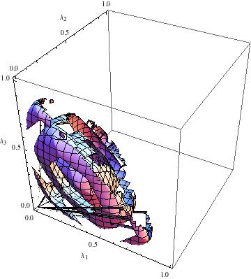
Figure 1: Three-dimensional contour plot of $VAD(\lambda_{1},\lambda_{2},\lambda_{3})$, given by eq. (8). Axes are of length 1.

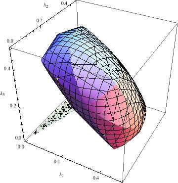
Figure 2: The absolutely separable boundary surface $VAD(\lambda_{1},\lambda_{2},\lambda_{3})=0$. Axes are of length $\frac{1}{2}$.

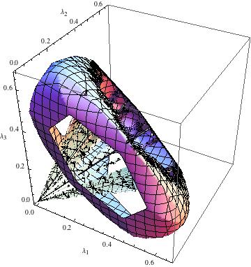
Figure 3: The surface corresponding to non-absolutely separable states with $VAD(\lambda_{1},\lambda_{2},\lambda_{3})=\frac{1}{3}$. Axes are of length $\frac{2}{3}$.

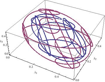
Figure 4: The blue points correspond to values of the (unsorted) eigenvalues for which the VAD bound on absolute separability (8) is equivalent to the ZHSL purity bound, $\lambda_{1}^{2}+\lambda_{2}^{2}+\lambda_{3}^{2}+\lambda_{4}^{2}\leq\frac{1}{3}$. The red points are those which satisfy the VAD bound, and for which the purity is, then, the greatest possible, that is, $\frac{3}{8}>\frac{1}{3}$.

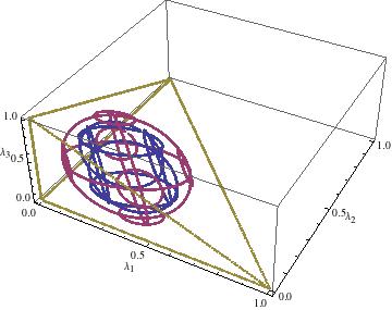
Figure 5: Fig. 4 embedded in the simplex of possible values of three (unordered) eigenvalues

It appeared to us that the ESF for the full 9-dimensional real and/or 15-dimensional complex convex sets of two-qubit states might be of the form,

$$\frac{2\sin^{-1}\left(U\right)}{\pi},$$ (11)

for $VAD(\lambda_{1},\lambda_{2},\lambda_{3})\geq 0$, and simply unity for $VAD(\lambda_{1},\lambda_{2},\lambda_{3})<0$.

II.2 Example 2

For our second example with one free Euler angle and three free eigenvalues, we set $x_{1}=x_{4}=x_{6}=\pi$ and $x_{2}=x_{3}=\frac{\pi}{2}$, allowing $x_{5}$ to be the free Euler angle now. (Scenarios with only one of $x_{2},x_{3},x_{4}$ or $x_{6}$ allowed to be free are trivially completely separable, and thus do not merit attention.) This results in density matrices of the form (again, taking $\lambda_{4}=1-\lambda_{1}-\lambda_{2}-\lambda_{3}$),

$$\left(\begin{array}[]{llll}\lambda_{3}\cos^{2}(x_{5})+\sin^{2}(x_{5})\lambda_{1}&0&0&\cos(x_{5})\sin(x_{5})\lambda_{3}-\cos(x_{5})\sin(x_{5})\lambda_{1}\\ 0&\lambda_{2}&0&0\\ 0&0&-\lambda_{1}-\lambda_{2}-\lambda_{3}+1&0\\ \cos(x_{5})\sin(x_{5})\lambda_{3}-\cos(x_{5})\sin(x_{5})\lambda_{1}&0&0&\lambda_{1}\cos^{2}(x_{5})+\sin^{2}(x_{5})\lambda_{3}\end{array}\right).$$ (12)

The Peres-Horodecki separability condition can now be expressed as

$$-\frac{1}{4}\sin^{2}\left(2x_{5}\right)\left(\lambda_{1}-\lambda_{3}\right){}^{2}-\lambda_{2}\left(\lambda_{1}+\lambda_{2}+\lambda_{3}-1\right)\geq 0.$$ (13)

In contrast to our first example, however, the (reduced) Haar measure (54) is now non-uniform, being $\sin{x_{5}}$. We, thus, sought to integrate this measure over the range $x_{5}\in[0,\pi]$, while enforcing the condition (13), to obtain the corresponding ESF. However, Mathematica did not yield a solution after what we judged to be a reasonable amount of computer time to expend.

Therefore, we made the transformation $x_{5}=\cos^{-1}\left(-y_{5}\right)$, which leads to a uniform measure for $y_{5}\in[-1,1]$. (There were some initial concerns expressed, in regard to this transformation, by S. Cacciatori. He had written: “The transformation you consider is not bijective on the whole range of the parameters. Indeed, the uniformization can be done only locally. This is because the measure on a compact manifold cannot be an exact form (otherwise, using Stokes Theorem, one finds zero volume for the manifold)” (cf. (Headrick and Wiseman, 2005, p. 4394)). However, subsequent analysis revealed that nothing fallacious arises in this manner, since the results are equivalent to twice those obtained by integrating over (the half-range) $y_{5}\in[0,1]$.) Now, the region of total separability was of the form,

$$\lambda_{1}<\frac{1}{2}\land\lambda_{1}>0\land\left(\left(2\lambda_{1}+\lambda_{2}>1\land(\text{M2}\lor\text{M3})\right)\lor(\text{M4}\land\text{M5})\right),$$ (14)

where

$$M2=\lambda_{1}+2\sqrt{\lambda_{2}-2\lambda_{1}\lambda_{2}}=2\lambda_{2}+\lambda_{3},M4=2\lambda_{2}+\lambda_{3}+2\sqrt{\lambda_{2}-2\lambda_{1}\lambda_{2}}>\lambda_{1},$$ (15)

$$M3=2\lambda_{2}+\lambda_{3}+2\sqrt{\lambda_{2}-2\lambda_{1}\lambda_{2}}>\lambda_{1}\land\lambda_{1}+2\sqrt{\lambda_{2}-2\lambda_{1}\lambda_{2}}\geq 2\lambda_{2}+\lambda_{3}$$ (16)

and

$$M5=\left(2\lambda_{1}+\lambda_{2}=1\land\lambda_{1}+\lambda_{2}+\lambda_{3}<1\right)\lor\left(\lambda_{2}>0\land\lambda_{1}+2\sqrt{\lambda_{2}-2\lambda_{1}\lambda_{2}}>2\lambda_{2}+\lambda_{3}\land 2\lambda_{1}+\lambda_{2}<1\right).$$ (17)

Also, non-trivially, the ESF took the (root) form

$$ESF_{\{x_{5}\}}(U)=\text{Root}\left[4\text{$\#$1}^{4}-4\text{$\#$1}^{2}+U^{2}\&,3\right]-\text{Root}\left[4\text{$\#$1}^{4}-4\text{$\#$1}^{2}+U^{2}\&,4\right]+1$$ (18)

(Root[$f,k$] represents the k-th root of the polynomial equation $f[x]=0$) for

$$2\lambda_{1}+\lambda_{2}>1\land 0<\lambda_{1}<\frac{1}{2}\land\lambda_{1}-2\lambda_{2}-\lambda_{3}+2\sqrt{\lambda_{2}-2\lambda_{1}\lambda_{2}}<0\land\lambda_{1}+\lambda_{2}+\lambda_{3}<1$$ (19)

or

$$\frac{1}{2}<\lambda_{1}<1\land\lambda_{1}+\lambda_{2}+\lambda_{3}<1\land\lambda_{2}>0.$$ (20)

In fact, (18) has an equivalent radical form,

$$ESF_{\{x_{5}\}}(U)=\frac{\sqrt{1-\sqrt{1-U^{2}}}}{\sqrt{2}}-\frac{\sqrt{1+\sqrt{1-U^{2}}}}{\sqrt{2}}+1.$$ (21)

The equivalence can be seen from a joint plot, in which (18) amd (21) fully coincide. However, the Mathematica command “ToRadicals” did not produce (21), but gave the sign of the second of the three addends as plus rather than minus. (“If Root objects in expr contain parameters, ToRadicals[expr] may yield a result that is not equal to expr for all values of the parameters”.) This was clearly an erroneous (“hyperseparable”–greater than 1) result. We initially had thought it might be due to an inappropriate uniformization, $x_{5}=\cos^{-1}\left(-y_{5}\right)$. (In Appendix II, we also give a derivation of S. Cacciatori of (21) “by hand”.) Therefore, we had also investigated alternative approaches to obtaining the required ESF.

We had reasoned that since the transformed VAD variable $U\equiv\frac{2\sqrt{\lambda_{2}\lambda_{4}}}{\lambda_{1}-\lambda_{3}}$ seemed to play a vital role, we performed the change-of-variables,

$$\left\{\lambda_{2}\to\frac{1}{2}\left(-\lambda_{1}-\lambda_{3}+\sqrt{\left(\lambda_{1}+\lambda_{3}-1\right){}^{2}-V\left(\lambda_{1}-\lambda_{3}\right){}^{2}}+1\right)\right\},$$ (22)

in our constrained integration analyses, where $V=U^{2}$. Now, we again imposed the nonascending-ordering requirement on the eigenvalues (and their transformed equivalents), and the Peres-Horodecki condition (13) (again discarding irrelevant nonnegative factors) became

$$2V+\cos\left(4x_{5}\right)-1\geq 0$$ (23)

(conveniently being free of the individual $\lambda$’s). Integrating the reduced Haar measure $\sin{x_{5}}$ over $x_{5}\in[0,\pi]$, while enforcing (23), we obtained the result (Fig. 6),

$$ESF_{\{x_{5}\}}(V)=\begin{cases}1&V>1\\ -\sqrt{1-\frac{1}{\sqrt{2}}}\cos\left(\frac{1}{4}\sin^{-1}(1-2V)\right)-\sqrt{1+\frac{1}{\sqrt{2}}}\sin\left(\frac{1}{4}\sin^{-1}(1-2V)\right)+1&0<V\leq 1.\end{cases}$$ (24)

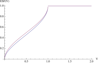
Figure 6: The eigenvalue-parameterized separability function given by eq. (24)—along with the slightly subordinate function, (11), $\frac{2\sin^{-1}\left(\sqrt{V}\right)}{\pi},V\in[0,1]$—for the real two-qubit scenario with the Euler angles $x_{1}=\pi,x_{2}=\frac{\pi}{2},x_{3}=\frac{\pi}{2},x_{4}=\pi,x_{6}=\pi$ and $x_{5}$ free. Here, $V=U^{2}=\frac{4\lambda_{2}\lambda_{4}}{(\lambda_{1}-\lambda_{3})^{2}}$, with $\lambda_{1}\geq\lambda_{2}\geq\lambda_{3}\geq\lambda_{4}$

We can represent this ESF more succinctly still, by using the variable $W=1-2V$. Then, we have

$$ESF_{\{x_{5}\}}(W)=\begin{cases}1&W<-1\\ 2\sin^{2}\left(\frac{1}{8}\cos^{-1}(W)\right)+\sin\left(\frac{1}{4}\cos^{-1}(W)\right)&-1\leq W<1\end{cases}.$$ (25)

III Absolute Separability Analyses

III.1 ZHSL uniform simplex measure

Verstraete, Audenaert and De Moor remarked that the use of their result (8) yields a better lower bound (assuming a uniform distribution on the simplex of eigenvalues) for the volume of separable states relative to the volume of all states: 0.3270 (as opposed to the ZHSL bound of 0.3023 based on the purity (Życzkowski et al., 1998, eq. (35))) (Verstraete et al., 2001, p. 6). We are now able to give exact formulas for these two bounds (certainly the second being new, and apparently somewhat challenging to derive), namely

$$ZHSL_{lower-bound}=\frac{\pi}{6\sqrt{3}}\approx 0.30229989$$ (26)

and (Figs. 1, 2 and 2)

$$VAD_{lower-bound}=\frac{1}{4}\left(8-6\sqrt{2}+3\sqrt{2}\tan^{-1}\left(\frac{1904\sqrt{2}}{5983}\right)\right)\approx 0.32723006.$$ (27)

The Verstraete-Audenaert-de Moor bound (8) is based on the entanglement of formation. They also present another bound (Verstraete et al., 2001, p. 2)

$$\tilde{VAD}(\lambda_{1},\lambda_{2},\lambda_{3})=\sqrt{(\lambda_{1}-\lambda_{3})^{2}+(\lambda_{2}-\lambda_{4})^{2}}-\lambda_{2}-\lambda_{4}<0,(\lambda_{1}>\lambda_{2}>\lambda_{3}>\lambda_{4}),$$ (28)

based on the negativity. (There is also a more complicated bound based on the relative entropy of entanglement. Since it involves logarithms, it is more difficult for us to analyze.) From this we obtained,

$$\tilde{VAD}_{lower-bound}=-\frac{12-8\sqrt{2}+3\pi+12\cot^{-1}\left(\frac{-6561+1904\sqrt{2}}{5983}\right)}{4\sqrt{2}}\approx 0.32723006,$$ (29)

fully equivalent, it would appear, to (27). (Perhaps it is clear that these two bounds (8) and (28) must be equivalent, though no explicit mention is made of this, it seems in Verstraete et al. (2001) nor the more recent Hildebrand (2007). Mathematica readily confirmed for us that there is no nontrivial domain in which one of the bounds is greater than 0 and the other one, less than 0.) Let us observe further, in regard to (29) that $6561=3^{8}$. Apparently, there is a right triangle with opposite legs of lengths 5983 and $1904\sqrt{2}$ and hypothenuse $6561=3^{8}$, that is of relevance in some way to the issue of the absolute separability of two-qubit states. We have consulted the Integer Superseeker website of N. J. A. Sloane (http://www.research.att.com/ njas/sequences) in regard to this issue, and found sequence A025172, entitled “ Let $\phi=\arccos{(\frac{1}{3})}$, the dihedral angle of the regular tetrahedron. Then $\cos{(n\phi)}=\frac{a(n)}{3^{n}}$”. In our application, $n=8$ and $a(n)=-5983$. The accompanying comment is that the sequence is “Used when showing that the regular simplex is not ‘scisssors-dissectable’ to a cube, thus answering Hilbert’s third problem.” Applying these facts to the problem at hand, we are able to obtain the simplified results

$$VAD_{lower-bound}=\tilde{VAD}_{lower-bound}=\frac{1}{4}\left(8-6\sqrt{2}+3\sqrt{2}\left(\pi-8\csc^{-1}(3)\right)\right)\approx 0.32723006.$$ (30)

We have obtained an area-to-volume ratio of (cf. Fig. 2)

$$R_{Area/Vol}=\frac{12\left(-1+3\sqrt{2}\cot^{-1}\left(2\sqrt{2}\right)\right)}{8-6\sqrt{2}+3\sqrt{2}\left(\pi-8\csc^{-1}(3)\right)}=\frac{12\left(-1+3\sqrt{2}\cot^{-1}\left(2\sqrt{2}\right)\right)}{8-6\sqrt{2}+3\sqrt{2}\pi-24\sqrt{2}\cot^{-1}\left(2\sqrt{2}\right)}\approx 4.050415.$$ (31)

III.2 HS measure on two-qubit real density matrices

Further, if we employ the Hilbert-Schmidt measure for two-rebit density matrices (Życzkowski and Sommers, 2003, eq. (7.5)) on the simplex of eigenvalues, we can obtain (V. Jovovic assisted with several trigonometric simplifications involving the dihedral angle, $\cos^{-1}(\frac{1}{3})$ an exact lower bound (much weaker than the conjectured actual value of $\frac{8}{17}\approx 0.470588$ (Slater, 2007b, sec. 9.1)) on the Hilbert-Schmidt two-qubit separability probability. This is

$$VAD_{HS-lower-bound}^{real}=\frac{6928-2205\pi}{16\sqrt{2}}\approx 0.0348338.$$ (32)

Also (cf. Szarek et al. (2006)),

$$R_{Area/Vol}^{HS-real}=\frac{1}{1287(-6928+2205\pi)}(\alpha_{1}+\alpha_{2})\approx 12.489976122,$$ (33)

where

$$\alpha_{1}=34087768\sqrt{2}-247867344\pi-1292769261\cos^{-1}\left(\frac{1}{3}\right)$$

and

$$\alpha_{2}=3226925088\cot^{-1}\left(\sqrt{2}\right)+3760128\tan^{-1}\left(\frac{1}{2\sqrt{2}}\right)+350082810\tan^{-1}\left(\sqrt{2}\right).$$

The corresponding ratio based on the Bures metric is modestly larger (as will also be the case in the corresponding complex and quaternionic scenarios), that is, 14.582. Multiplying (33) by the radius–$\frac{1}{12}$–of the maximal ball inscribed inside the simplex of eigenvalues, we obtain a dimensionless ratio, $\gamma\approx 3.60555$ (Szarek et al., 2006, eq. (1)) (cf. Innami (1999)).

III.3 HS measure on two-qubit complex density matrices

We have also obtained an exact expression for the HS absolute separability probability of generic (complex) two-qubit states (using the indicated measure (Życzkowski and Sommers, 2003, eq. (3.11))),

$$VAD_{HS-lower-bound}^{complex}=\frac{\psi_{1}+\psi_{2}}{32614907904}\approx 0.0036582630543035$$ (34)

where

$$\psi_{1}=1959684729929728-1601255307608064\sqrt{2}-1529087492782080\sqrt{2}\pi$$

and

$$\psi_{2}=45247615492565918250\sqrt{2}\cot^{-1}\left(\sqrt{2}\right)-22619730179635540245\sqrt{2}\sec^{-1}(3).$$

(The conjectured HS [absolute and non-absolute] separability probability of generic two-qubit complex states is $\frac{8}{33}\approx 0.242424$ (Slater, 2007b, sec. 9.2).) Further, we have

$$R_{Area/Vol}^{HS-complex}=-3840\frac{\tau_{1}+\tau_{2}}{\tau_{3}+\tau_{4}}\approx 20.9648519,$$ (35)

with

$$\tau_{1}=-5358569267936+33756573946095\sqrt{2}\pi-270052591568760\sqrt{2}\cot^{-1}\left(\sqrt{2}\right),$$

$$\tau_{2}=11149704525960\sqrt{2}\cot^{-1}\left(2\sqrt{2}\right)+270052591568760\sqrt{2}\cot^{-1}\left(3+\sqrt{2}\right),$$

$$\tau_{3}=-1959684729929728+1601255307608064\sqrt{2}+1529087492782080\sqrt{2}\pi,$$

and

$$\tau_{4}=-45247615492565918250\sqrt{2}\cot^{-1}\left(\sqrt{2}\right)+22619730179635540245\sqrt{2}\sec^{-1}(3).$$

The corresponding dimensionless ratio is $\gamma\approx 6.05203$, while the Bures analogue of (35) is 23.7826.

Employing the Bures measure (Sommers and Życzkowski, 2003, eq. (3.18)) for generic two-qubit states on the simplex of eigenvalues, we have, numerically, a lower bound–based on the absolutely separable states–on the two-qubit Bures separability probability of 0.000161792, considerably smaller than the conjectured value of $\frac{1680(\sqrt{2}-1)}{\pi^{8}}\approx 0.0733389$ Slater (2005a).

III.4 HS measure on two-qubit quaternionic density matrices

The HS absolute separability probability of the quaternionic two-qubit states is

$$VAD_{HS-lower-bound}^{quat}=-\frac{13}{816946343106356485029888}\Sigma_{i=1}^{6}\zeta_{i}\approx 0.000039870347068,$$ (36)

(the conjectured absolute and non-absolute separability probability being $\frac{72442944}{936239725}\approx 0.0773765$ (Slater, 2008, eq. (15))), where

$$\zeta_{1}=-216449750678398795533760757497856+176860737736399592490919645937664\sqrt{2},$$

$$\zeta_{2}=279292548969739228073088142369304501839785\sqrt{2}\pi$$

$$\zeta_{3}=-558572941247617043110461841280869072896000\sqrt{2}\cot^{-1}\left(\sqrt{2}\right),$$

$$\zeta_{4}=23637916932187025487103667523337320\sqrt{2}\cot^{-1}\left(2\sqrt{2}\right),$$

$$\zeta_{5}=-16178155879591789043088455851252390200\sqrt{2}\cot^{-1}\left(3+\sqrt{2}\right)$$

$$\zeta_{6}=-558589165778586158484606527963549721006600\sqrt{2}\tan^{-1}\left(\sqrt{2}\right).$$

Additionally,

$$R_{Area/Vol}^{HS-quat}=\frac{13}{3606947894919168V^{quat}}(\psi_{1}+\psi_{2})\approx 37.9283799507,$$ (37)

where $V^{quat}$ is given by (36) and

$$\psi_{1}=-18147776040854148031593056-4720063928074960763823525\sqrt{2}\pi,$$

and

$$\psi_{2}=-37760511424599686110588200\sqrt{2}\tan^{-1}\left(9-7\sqrt{2}\right).$$

The corresponding dimensionless ratio is $\gamma\approx 10.948980$, and the Bures area-to-volume ratio counterpart to (37) is–slightly higher as in the real and complex cases–42.115.

III.4.1 Two-qubit Clément-Raggio spectral condition

Clément and Raggio have given a simple (linear) spectral condtion that ensures separability of two-qubit states (Clément and Raggio, 2006, Thm. 1),

$$3\lambda_{1}+\sqrt{2}\lambda_{2}+(3-\sqrt{2})\lambda_{3}\leq 2,\hskip 36.135pt\lambda_{1}\geq\lambda_{2}\geq\lambda_{3}.$$ (38)

Based on this, we readily found–using the ZHSL uniform measure on the simplex of eigenvalues–that a lower bound on the separability probability is $\frac{1}{3\sqrt{2}}\approx 0.235702$, and the area-to-volume ratio is 6.

Now if we employed the HS measure for the real density matrices, along with the spectral condition (38), the lower bound is $\frac{104+75\sqrt{2}}{17496}\approx 0.0120065$ and the area-to-volume ratio, 18. The corresponding two figures in the HS complex measure case are $0.00060239769$ and 30, and, in the quaternionic case, $1.502473896\cdot 10^{-6}$ and 54.

Clément and Raggio also gave a spectral separability condition applicable to any finite-dimensional system, but “much weaker” than (38) in the specific two-qubit case (Clément and Raggio, 2006, Thm. 2). In the two-qubit case, it takes the form,

$$3\lambda_{3}+3\lambda_{4}\geq 1,\hskip 36.135pt\lambda_{3}\geq\lambda_{4}.$$ (39)

Based on this constraint, the lower bound on the separability probability using the ZHSL uniform measure is $\frac{1}{9}\approx 0.11111$, while the area-to-volume ratio is 6. The associated separability probability based on the HS measure on the real density matrices is $\frac{7}{6561}\approx 0.00106691$ and area-to-volume ratio, 18. The corresponding HS complex measure values are $\frac{143}{14348907}\approx 9.96592\cdot 10^{-6}$ and 30, while the two quaternionic values are $\frac{2185}{2541865828329}\approx 8.59605\cdot 10^{-10}$ and 54.

We see that the four area-to-volume ratios given are identical using either of the two bounds (38) and (39), that is, 6, 18, 30 and 54..

III.5 Qubit-Qutrit analyses

The counterpart of the VAD bound (8) for qubit-qutrit states was obtained by Hildebrand (Hildebrand, 2007, eq. (4)) (Fig. 7)

$$H(\lambda_{1},\lambda_{2},\lambda_{3},\lambda_{4},\lambda_{5})=\lambda_{1}-\lambda_{5}-2\sqrt{\lambda_{4}\lambda_{6}}<0,\hskip 10.84006pt(\lambda_{1}>\lambda_{2}>\lambda_{3}>\lambda_{4}>\lambda_{5}>\lambda_{6}).$$ (40)

Figure 7: Three-dimensional projection of the sets of six (unsorted) eigenvalues, $\lambda_{i},=1,\ldots,6$, for which the Hildebrand bound (40) on absolute separability of qubit-qutrit systems is equivalent to the ZHSL purity bound $\Sigma_{i}^{6}\lambda_{i}^{2}\leq\frac{1}{5}$ (cf. Figs. 4 and 5).

We have also sought to obtain exact lower bounds on separability probabilities here, using (40). Discouragingly, however, it seemed, after some initial analyses that computer memory demands may be too great to make any significant analytical progress on the full five-dimensional problem. (Nor have we been able to determine–as we have in the qubit-qubit case (after (9))–the maximum values that the $\lambda_{i}$’s can attain for absolutely separable states.) However, we then sought to reduce/specialize the problem to more computationally manageable forms.

Firstly, we found that if we set $\lambda_{1}=\frac{1}{3}$, then the absolute separability probability employing the uniform measure on the resulting four-dimensional simplex is 0.00976679. (The corresponding value for the full five-dimensional simplex was reported by ZHSL as 0.056 (Życzkowski et al., 1998, eq. (35)).) However, this probability jumps dramatically to 0.733736, if we reduce $\lambda_{1}$ from $\frac{1}{3}$ to $\frac{1}{4}$.

III.5.1 Clément-Raggio spectral conditions

We did succeed, however, in this qubit-qutrit case in terms of the “simple spectral condition” of Clément and Raggio (Clément and Raggio, 2006, Thm. 2), which in our case takes the form,

$$3\lambda_{6}+5\lambda_{5}\geq 1,\hskip 36.135pt\lambda_{5}\geq\lambda_{6}.$$ (41)

The resultant bound on the ZHSL separability probability (based on the uniform measure over the simplex) is, then, quite elegantly, $\frac{1}{256}=2^{-8}$, and the associated area-to-volume ratio is simply 15. Additionally, we found that the lower bound for the separability probability based on the HS measure for real density matrices is

$$\frac{18989}{214748364800000}\approx 8.842442\cdot 10^{-11}.$$ (42)

Again, we have a simple area-to-volume ratio, 60.

IV Discussion

We have attempted, so far without success, to obtain exact ESFs with more than one free Euler angle. In particular, we have tried to “combine” the two one-free-Euler-angle scenarios analyzed above, by letting both $x_{1}$ and $x_{5}$ be free. The associated Peres-Horodecki separability criterion (cf. (2), (13)) is then,

$$\left(\lambda_{3}\cos^{2}\left(x_{5}\right)+\sin^{2}\left(x_{5}\right)\lambda_{1}\right)\left(\lambda_{1}\cos^{2}\left(x_{5}\right)+\sin^{2}\left(x_{5}\right)\lambda_{3}\right)-\frac{1}{4}\sin^{2}\left(2x_{1}\right)\left(\lambda_{1}+2\lambda_{2}+\lambda_{3}-1\right){}^{2}\geq 0.$$ (43)

The best we were able to achieve, having first integrated over $x_{5}\in[0,\pi]$, was a finding that the ESF for this two-Euler-angle scenario (again assuming $\lambda_{1}\geq\lambda_{2}\geq\lambda_{3}\geq\lambda_{4}$) is expressible as

$$ESF_{\{x_{1},x_{5}\}}(\lambda_{1},\lambda_{2},\lambda_{3})=\int_{0}^{2\pi}\begin{cases}1&\kappa\geq 1\\ \cos\left(\frac{1}{4}\cos^{-1}(\kappa)\right)-\sin\left(\frac{1}{4}\cos^{-1}(\kappa)\right)&-1<\kappa<1\end{cases}dx_{1}$$ (44)

where

$$\kappa=\frac{\cos\left(4x_{1}\right)\left(\lambda_{1}+2\lambda_{2}+\lambda_{3}-1\right){}^{2}+4\lambda_{2}+2\lambda_{3}-4\lambda_{2}\left(\lambda_{2}+\lambda_{3}\right)+\lambda_{1}\left(-4\lambda_{2}+4\lambda_{3}+2\right)-1}{\left(\lambda_{1}-\lambda_{3}\right){}^{2}}.$$ (45)

Alternatively, we were able to reduce this two-free-Euler-angle problem to

$$ESF_{\{x_{1},x_{5}\}}(\lambda_{1},\lambda_{2},\lambda_{3})=\int_{0}^{\pi}\sin{x_{5}}\begin{cases}1&\eta>1\\ \frac{\sin^{-1}(\eta)}{\pi}+\frac{1}{2}&-1<\eta\leq 1,\end{cases}dx_{5}$$ (46)

where

$$\eta=\frac{-\cos\left(4x_{5}\right)\left(\lambda_{1}-\lambda_{3}\right){}^{2}+4\lambda_{2}+2\lambda_{3}-4\lambda_{2}\left(\lambda_{2}+\lambda_{3}\right)+\lambda_{1}\left(-4\lambda_{2}+4\lambda_{3}+2\right)-1}{\left(\lambda_{1}+2\lambda_{2}+\lambda_{3}-1\right){}^{2}}.$$ (47)

On the other hand, we have not yet found an exact ESF with even just one free Euler angle using the Tilma-Byrd-Sudarshan $SU(4)$ parameterization Tilma et al. (2002) of the 15-dimensional convex set of (in general, complex) $4\times 4$ density matrices. Further, we have been able to convince ourselves–somewhat disappointingly–that the ESF for the real $4\times 4$ density matrices can not simply be a (univariate) function of $V$ (or $U$)–such as (11). We were able to reach this conclusion by finding distinct sets of eigenvalues ($\lambda_{1},\lambda_{2},\lambda_{3},\lambda_{4}$), which yielded the same identical value of $V$ (we used $V=\frac{1}{2}$), but were capable of giving opposite signs for the determinant of the partial transpose, when sets of six (randomly-chosen) Euler angles were held fixed.

The analyses we have presented above have considerable similarities in purpose with a notable study of Batle, Casas and A. and A. R. Plastino, “On the entanglement properties of two-rebit systems” Batle et al. (2002) (cf. Batle et al. (2006)). Some differences between our work and theirs are that we have employed the Verstraete-Audenaert-de Moor entanglement measure (8) and its transforms ($U$ and $V$) rather than the purity (which gives a smaller domain of absolute separability), and we have striven to obtain exact analytical results, rather than numerical ones (cf. (Slater, 2008, sec. 3)). (Let us note, in passing–although we have not adopted this viewpoint here–“that there is qualitative difference between the separability problems for real and complex matrices. In fact, the set of separable density matrices has the same dimension as the full set of density matrices in the complex case, but has lower dimension in the real case” (Dahl et al., 2007, p. 713).)

We have been principally concerned here (sec. II) with the generation (by integration of the Haar measure over the Euler angles) of metric-independent eigenvalue-parameterized separability functions (ESFs). Such ESFs could be applied, in conjunction with the formulas for arbitrary metrics (e. g. (Życzkowski and Sommers, 2003, eq. (4.1)), (Sommers and Życzkowski, 2003, eq. (3.18)) (Bengtsson and Życzkowski, 2006, eqs. (14.34), (14.45))) to yield separability probabilities specific to the metrics in question.

We have also reported (sec. III) advances in the study of absolute separability, implementing the Verstraete-Audenaert-de Moor bound (8). A substantial analytical challenge in regard to this is the determination of the volumes and bounding areas (and their ratios) of the absolutely separable two-qubit states in terms of the Bures (minimal monotone) metric. (We have given numerical values of these ratios above.) We have derived several remarkable exact trigonometric formulas pertaining to absolute separability. (V. Jovovic has assisted us in this task, simplifying Mathematica output by using identities involving the tetrahedral dihedral angle $\phi=\cos^{-1}\left(\frac{1}{3}\right)$.) Nevertheless, we can certainly not ensure that further (conceivably substantial) simplifications exist.

V Appendix I (S. Cacciatori)

The Lie algebra $so(4)$ of $SO(4)$ consists of the $4\times 4$ antisymmetric real matrices. A basis is given by the following matrices:

$$T_{1}=\left(\begin{array}[]{cccc}0&1&0&0\\ -1&0&0&0\\ 0&0&0&0\\ 0&0&0&0\end{array}\right)$$

$$T_{2}=\left(\begin{array}[]{cccc}0&0&1&0\\ 0&0&0&0\\ -1&0&0&0\\ 0&0&0&0\end{array}\right)$$

$$T_{3}=\left(\begin{array}[]{cccc}0&0&0&0\\ 0&0&1&0\\ 0&-1&0&0\\ 0&0&0&0\end{array}\right)$$

$$T_{4}=\left(\begin{array}[]{cccc}0&0&0&1\\ 0&0&0&0\\ 0&0&0&0\\ -1&0&0&0\end{array}\right)$$

$$T_{5}=\left(\begin{array}[]{cccc}0&0&0&0\\ 0&0&0&1\\ 0&0&0&0\\ 0&-1&0&0\end{array}\right)$$

$$T_{6}=\left(\begin{array}[]{cccc}0&0&0&0\\ 0&0&0&0\\ 0&0&0&1\\ 0&0&-1&0\end{array}\right)$$

. The maximal proper subgroup of $SO(4)$ is $SO(3)$ and can be thought of as the isotropy subgroup of $SO(4)$. This means that if we consider $SO(4)$ as the group of rotations of $\mathbb{R}^{4}$, then this group acts transitively on the unit sphere (translating the north pole everywhere on the sphere), but any point is left fixed by the subgroup $SO(3)$. Thus we will have

$$SO(4)/SO(3)\simeq S^{3}.$$

This is the main observation needed to determine the range of the parameters.
Now let us look at the construction of the Euler parametrisation of the group. First, one searches for a maximal subgroup, in our case $H=SO(3)$. (In general, this might be not unique: for example for $E_{6}$ we have chosen $F_{4}$ as a maximal subgroup, but another possible choice could have been $U(1)\times Spin(10)$). We can suppose that we know the Euler parametrisation for the subgroup. Otherwise, we can proceed inductively, choosing a subgroup for $H$ and so on.
In our case for $H$, we can choose the $SO(3)$ subgroup generated by $T_{i}$, $i=1,2,3$. The Euler parametrisation of $H=SO(3)$ is well known,

$$h[x,y,z]=e^{xT_{3}}e^{yT_{2}}e^{zT_{3}}\ .$$

To determine the range of the parameters we first note that $SO(3)$ is not simply connected, but its universal covering is $SU(2)$ and $SO(3)\simeq SU(2)/{\{I,-I\}}$ ($I$ being the identity). Also, it is well known that $SU(2)\simeq S^{3}$ as a manifold. With this in mind, let us compute the invariant metric (and measure) on $H$. This can be done, noting that the Lie algebra is isomorphic to the tangent space at the identity $e$ of the group. But our algebra is provided by a natural scalar product, the trace product

$$\langle\ ,\rangle:so(4)\times so(4)\longrightarrow\mathbb{R},$$

$$\qquad(A,B)\longmapsto-\frac{1}{2}{\rm Trace}(AB)\ .$$

It is symmetric and positive definite, satisfies

$$\langle T_{I},T_{J}\rangle=\delta_{IJ}$$

and induces a Euclidean scalar product on $T_{e}H$, with $\langle T_{i},T_{j}\rangle=\delta_{ij}$. Thus, it is easy to compute the metric on $H$ as the metric induced by the scalar product on $T_{e}H$. Indeed, if $h[x,y,z]$ is a generic point, then $dh$ is cotangent at the point $h$ and $h^{-1}dh$ is cotangent at $e$, so that the metric tensor can be defined as

$$ds_{H}^{2}=\langle h^{-1}dh,h^{-1}dh\rangle=-\frac{1}{2}{\rm Trace}(h^{-1}dhh^{-1}dh)\ .$$

From this expression, we immediately see that $ds_{H}^{2}$ is both left and right invariant. A direct computation gives

$$ds_{H}^{2}=dx^{2}+dy^{2}+dz^{2}+2\cos(y)dxdz.$$

Now we need to compare this with the metric of a sphere $S^{3}$. This can be done, describing $S^{3}$ as the unit sphere in $\mathbb{C}^{2}$,

$$S^{3}=\{(z,w)\in\mathbb{C}^{2}|z\bar{z}+w\bar{w}=1\}.$$

Then, the point $p$ of $S^{3}$ can be parametrised as

$$p=(\cos\lambda e^{i(\phi+\psi)},\sin\lambda e^{i(\phi-\psi)})$$

covered by $\lambda\in[0,\pi/2]$, $\phi\in[0,\pi]$, $\psi\in[0,2\pi]$. The Euclidean metric is

$$ds^{2}=dzd\bar{z}+dwd\bar{w}=d\lambda^{2}+d\phi^{2}+d\psi^{2}+2\cos(2\lambda)d\phi d\psi.$$

Comparing this with the invariant metric, we see that it is the metric of $S^{3}$ with $y=2\lambda$, $x=2\phi$ and $z=2\psi$ (note that $x$ and $z$ can be symmetrically interchanged). Now if we impose on $x,y,z$ the ranges for the sphere, that is

$$x\in[0,2\pi],\qquad y\in[0,\pi],\qquad z\in[0,4\pi],$$

we will cover $SO(3)$ exactly two times. This is because $SO(3)\simeq S^{3}/{\pm I}$ as noted before. However, we can easily check where duplication takes place. Indeed,

$$e^{zT3}=\left(\begin{array}[]{cccc}1&0&0&0\\ 0&\cos z&\sin z&0\\ 0&-\sin z&\cos z&0\\ 0&0&0&1\end{array}\right)$$

and takes all possible values twice when $z$ varies in $[0,4\pi]$. The correct range is then

$$x\in[0,2\pi],\qquad y\in[0,\pi],\qquad z\in[0,2\pi].$$

Now we are ready to construct the group $G=SO(4)$. Any element of $G$ can be written in the form

$$e^{xT_{4}+yT_{5}+zT_{6}}h[x_{4},x_{5},x_{6}].$$

This is shown in an appendix of our paper on $F_{4}$ Bernardoni et al. . Here $(x,y,z)$ varies in $\mathbb{R}^{3}$. (We are not concerned at this level with the possibility of covering the group many times. The only important point is that this parametrisation is surjective). Now, we note that $H$ acts on $T_{a}$, as the rotations of $SO(3)$ act on the points of the unit sphere $S^{2}$. In particular, from

$$[T_{2},T_{4}]=-T_{6},\qquad[T_{2},T_{6}]=T_{4},\qquad[T_{3},T_{4}]=0,\qquad[T_{3},T_{6}]=T_{5},\qquad[T_{3},T_{5}]=-T_{6}$$

we find

$$e^{xT_{2}}T_{4}e^{-xT_{2}}=\cos xT_{4}-\sin xT_{6}\ ,$$

$$e^{yT_{3}}e^{xT_{2}}T_{4}e^{-xT_{2}}e^{-yT_{3}}=\cos xT_{4}-\sin x\cos yT_{6}-\sin x\sin yT_{5}.$$

Because any vector in $\mathbb{R}^{3}$ can be written as

$$\vec{x}=r(\cos x,-\sin x\sin y,-\sin x,\cos y),$$

and because

$$ga^{A}g^{-1}=e^{gAg^{-1}},$$

we can write

$$e^{xT_{4}+yT_{5}+zT_{6}}=e^{x_{1}T_{3}}e^{x_{2}T_{2}}e^{x_{3}T_{4}}e^{-x_{2}T_{2}}e^{-x_{1}T_{3}}$$

for some $x_{1},x_{2}$ and $x_{3}(=r)$. Moreover, $e^{-x_{2}T_{2}}e^{-x_{1}T_{3}}\in H$, so that we can reabsorb it into $h$ and write the general point on $SO(4)$ as

$$g[x_{1},\ldots,x_{6}]=e^{x_{1}T_{3}}e^{x_{2}T_{2}}e^{x_{3}T_{4}}h[x_{4},x_{5},x_{6}].$$

We know the range for the parameters $x_{4},x_{5},x_{6}$. To determine the ranges for the remaining parameters, we note that

$$p[x_{1},x_{2},x_{3}]=e^{x_{1}T_{3}}e^{x_{2}T_{2}}e^{x_{3}T_{4}},$$

parametrises the points of $SO(4)/SO(3)=S^{3}$, so that we need to compute the metric induced on $SO(4)/SO(3)$ and compare it with the metric of $S^{3}$. As before, we need to compute the left invariant form

$$J_{P}:=P^{-1}dP.$$

However, in general, $J_{P}$ is not cotangent to $P$, because $P$ is not a subgroup, so that it will have a component tangent to the fiber $H$. Fortunately, our choice for the product separates $P$ from $H$ orthogonally, and we can obtain the infinitesimal displacement along $P$ by an orthogonal projection (that is dropping the terms $T_{i}$, $i=1,2,3$). If we call such a projection $\Pi$, we, thus, have

$$ds^{2}_{P}=-\frac{1}{2}{\rm Trace}(\Pi(J_{P})\Pi(J_{P})),$$

where

$$J_{P}=dx_{3}T_{4}-\sin x_{3}dx_{2}T_{6}-\sin x_{2}\sin x_{3}T_{5}dx_{1}+\ldots,$$

the dots indicating the terms tangent to $H$. Thus, we get

$$ds^{2}_{P}=dx_{3}^{2}+\sin^{2}x_{3}(dx_{2}^{2}+\sin^{2}x_{2}dx_{1}^{2}),$$

which is just the metric of $S^{3}$ in the usual spherical polar coordinates,

$$S^{3}=\{X\in\mathbb{R}^{4}|X_{1}=\cos x_{3},\ X_{2}=\sin x_{3}\cos x_{2},\ X_{3}=\sin x_{3}\sin x_{2}\cos x_{1},\ X_{4}=\sin x_{3}\sin x_{2}\sin x_{1}\},$$

so that we must choose

$$x_{3}\in[0,\pi],\qquad x_{2}\in[0,\pi],\qquad x_{3}\in[0,2\pi].$$

This complete our determination of the ranges.

The invariant measure is

$$d\mu_{SO(4)}=\sqrt{{\rm det}ds^{2}_{H}}\sqrt{{\rm det}ds^{2}_{P}}=\sin x_{2}\sin^{2}x_{3}\sin x_{5}dx_{1}dx_{2}dx_{3}dx_{4}dx_{5}dx_{6}.$$ (54)

Note that there is a second quite interesting way to determine the ranges using the measure. To understand it, let us think of a sphere $S^{2}$ parametrised with latitudinal and longitudinal (polar) coordinates. But suppose we do not know the ranges of parameters. The only fact we know is that we can cover our sphere entirely, if any coordinate runs over a whole period ($\lambda\in[0,2\pi]$, $\phi\in[0,2\pi]$). The problem is that we can cover the sphere many times (twice in our case). But suppose we know the corresponding measure: $|\sin\lambda|d\lambda d\phi$. We see that it becomes singular at $\lambda=0$ and $\lambda=\pi$. These correspond to the points where the parallels shrink down (that is, the north and south poles). This implies that when $\lambda$ runs over $[0,\pi]$, we generate a closed surface which, thus, must cover the sphere (which contains no closed surfaces but itself), so that the range of $\lambda$ can be restricted to $[0,\pi]$.
In the same way, we can look at the invariant metric we have just constructed for $SO(4)$. All coordinates $x_{I}$, $I=1,\ldots,6$ have period $[0,2\pi]$ because the $\exp(x_{I}T_{I})$ are functions of $\cos x_{I}$ and $\sin x_{I}$. However, $x_{2}$, $x_{3}$ and $x_{5}$ appear in the measure exactly as for the sphere and must be restricted to $[0,\pi]$. Thus, we re-obtain the ranges

$$x_{1},x_{4},x_{6}\in[0,2\pi],\qquad x_{2},x_{3},x_{5}\in[0,\pi].$$ (55)

VI Appendix II (S. Cacciatori)

Let us call $\Delta$ the eigenvalues simplex and $M$ the subset of varying angles for the chosen example. Finally let us call $S$ the subset of $M$ imposed by the Peres-Horodecki condition (13)

$$-\frac{1}{4}\sin^{2}\left(2x_{5}\right)\left(\lambda_{1}-\lambda_{3}\right){}^{2}-\lambda_{2}\left(\lambda_{1}+\lambda_{2}+\lambda_{3}-1\right)\geq 0.$$ (56)

Thus we need to compute

$$ESF_{\{x_{5}\}}=\int_{S}d\mu/\int_{M}d\mu$$ (57)

$d\mu$ being the measure on the given region. In particular (13) constraints the range of $x_{5}$ only, so that

$$ESF_{\{x_{5}\}}=\frac{1}{2}\int_{S}\sin x_{5}dx_{5}.$$ (58)

Note that (13) is invariant under $x_{5}\rightarrow\pi-x_{5}$ so that we can restrict the region $S$ to $S_{0}=S\cap[0,\pi/2]$ and write

$$ESF_{\{x_{5}\}}=\int_{S_{0}}\sin x_{5}dx_{5}.$$ (59)

Furthermore, in $[0,\pi/2]$ the map $y_{5}=\sin x_{5}$ is bijective as a map $[0,\pi/2]\rightarrow[0,1]$ so that we can write

$$ESF_{\{x_{5}\}}=\int_{\sigma}dy_{5},$$ (60)

where $\sigma$ is the set of solutions of

$$-y_{5}^{2}(1-y_{5}^{2})\left(\lambda_{1}-\lambda_{3}\right){}^{2}+\lambda_{2}\lambda_{4}\geq 0,$$ (61)

in $[0,1]$, $\lambda_{4}=1-\lambda_{1}-\lambda_{2}-\lambda_{3}$. To determine $\sigma$ let us first set $z=y_{5}^{2}$. The solutions of

$$(z^{2}-z)\left(\lambda_{1}-\lambda_{3}\right){}^{2}+\lambda_{2}\lambda_{4}=0,$$ (62)

are

$$z_{\pm}=\frac{1}{2}\left[1\pm\sqrt{1-\frac{4\lambda_{2}\lambda_{4}}{(\lambda_{1}-\lambda_{3})^{2}}}\right].$$ (63)

When the discriminant is non positive, that is when $(\lambda_{1}-\lambda_{3})^{2}\leq 4\lambda_{2}\lambda_{4}$, then (61) is satisfied for all $y$ and $ESF=1$. Otherwise $z_{\pm}$ satisfy

$$0\leq z_{-}<z_{+}\leq 1.$$ (64)

In this case

$$(z^{2}-z)\left(\lambda_{1}-\lambda_{3}\right){}^{2}+\lambda_{2}\lambda_{4}\geq 0,$$ (65)

is solved for external values and being $z\in[0,1]$ we have that (61) is satisfied for

$$z\in[0,z_{-}]\cup[z_{+},1],$$ (66)

and then (being again $\sqrt{z}=y_{5}\in[0,1]$)

$$y_{5}\in[0,\sqrt{z_{-}}]\cup[\sqrt{z_{+}},1]\equiv\sigma.$$ (67)

Thus

$$ESF_{\{x_{5}\}}=1-\sqrt{z_{+}}+\sqrt{z_{-}}=1-\frac{\sqrt{1+\sqrt{1-U^{2}}}}{\sqrt{2}}+\frac{\sqrt{1-\sqrt{1-U^{2}}}}{\sqrt{2}}.$$ (68)