The Dark Matter Constraints on the Left-Right Symmetric Model with $Z_{2}$ Symmetry

Abstract

In the framework of Left-Right symmetric model, we investigate an interesting scenario, in which the so-called VEV seesaw problem can be naturally solved with $\cal{Z}$₂ symmetry. In such a scenario, we find a pair of stable weakly interacting massive particles (WIMPs), which may be the cold dark matter candidates. However, the WIMP-nucleon cross section is 3-5 orders of magnitude above the present upper bounds from the direct dark matter detection experiments for $m\sim 10^{2}-10^{4}$ GeV. As a result, the relic number density of two stable particles has to be strongly suppressed to a very small level. Nevertheless, our analysis shows that this scenario can’t provide very large annihilation cross sections so as to give the desired relic abundance except for the resonance case. Only for the case if the rotation curves of disk galaxies are explained by the Modified Newtonian Dynamics (MOND), the stable WIMPs could be as the candidates of cold dark matter.

I Introduction

The Left-Right (LR) symmetric model LR , based on the gauge group $SU(2)_{L}\times SU(2)_{R}\times U(1)_{B-L}$, is an attractive extension of the standard model (SM). The symmetry requires the introduction of right-handed partners for the observed gauge bosons and neutrinos, and a Higgs sector containing one bi-doublet $\phi$ (2,2,0), one left-handed triplet $\Delta_{L}$ (3,1,2) and one right-handed triplet $\Delta_{R}$ (1,3,2). In such a minimal LR symmetric model, parity is an exact symmetry of the theory at high energy scale, and is broken spontaneously at low energy scale due to the asymmetric vacuum. Also CP asymmetry can be realized as a consequence of spontaneous symmetry breaking, namely the spontaneous CP violation (SCPV) SCPV . However, such a scenario suffers from nontrivial constraints from the vacuum minimization conditions. It is explicitly demonstrated that the SCPV is not so easily realized if all the parameters in the Higgs potential are real and endowed with natural values Mohapatra ; VEV ; Barenboim . The difficulty results from the facts that one of the neutral Higgs bosons carries dangerous tree level flavor changing neutral currents (FCNC) effect, and that quark flavor mixing angles and CP violating phase are all calculable quantities due to the LR symmetry. Therefore, many generalized CP violation scenarios beyond the SCPV case have been analyzed extensively Langacker ; Bernabeu ; Pos ; Frere ; Kie ; Ji . In these literatures, the masses of right-handed gauge boson $W_{2}$ and the FCNC Higgs boson are strongly constrained from low energy phenomenology. Although the CKM matrix are more general not to be fully fixed than the SCPV case, it is proved that there is only one physical complex phase in the Yukawa couplings Ken . Hence the FCNC Higgs boson’s couplings can’t be absolutely free. The FCNC Higgs boson’s mass still accepts strict bound. In terms of these observations, a generalized two Higgs bi-doublets model is proposed Wu . In this model, quark mass matrices become far more flexible and the FCNC Higgs boson’s Yukawa couplings are now free parameters. Thereby low energy bound on the right-handed scale is largely alleviated. As other generalized models, the two Higgs bi-doublets version of LR model also has the advantage to realize the SCPV without the fine-tuning problem.

The LR symmetric model is also motivated to explain the very tiny neutrino masses. When the vacuum expectation value (VEV) $v_{R}$ of the neutral component of $\Delta_{R}$ is very huge, typically of order $10^{12}$ GeV, the well-known seesaw mechanism provides a very natural explanation of the smallness of neutrino masses SEESAW . However, the right-handed gauge bosons $Z_{2}$ and $W_{2}$ are too heavy to be detected at the Large Hadron Collider (LHC) and the future colliders. To allow for the possibility of an observable right-handed scale, many authors focus on the $v_{R}\sim 10$ TeV case. Although the seesaw mechanism can work well, we have to face the so-called VEV-seesaw puzzle. Namely, $\beta/\rho$ is of order $10^{-10}$ rather than the anticipant ${\cal O}(1)$, where $\rho$ and $\beta$ are located in the Higgs potential. One may introduce a discrete ${\cal Z}_{2}$ symmetry $\Delta_{L}\rightarrow-\Delta_{L}$ and $\Delta_{R}\rightarrow\Delta_{R}$ to resolve this VEV-seesaw problem VEV . It is worthwhile to stress that neutrinos are the Dirac particles in this scenario. If we preserve the Majorana Yukawa couplings, the corresponding model must lie beyond the LR symmetric model.

The ${\cal Z}_{2}$ symmetry leads to the absence of both $\beta$-type terms and the Majorana Yukawa couplings, hence $v_{L}=0$ due to the minimization conditions. Furthermore, we find that the neutral Higgs bosons $\delta_{L}^{0}$ and ${\delta_{L}^{0}}^{*}$ are a pair of stable weakly interacting massive particles (WIMPs). This is an important feature of our scenario which hasn’t been indicated before. It is a natural idea that $\delta_{L}^{0}$ and ${\delta_{L}^{0}}^{*}$ may be the cold dark matter candidates DM . We firstly calculate the WIMP-nucleon elastic scattering cross section which has been strongly constrained by the direct dark matter detection experiments, such as the CDMSCDMS and XENONXENON . However, our result is 3-5 orders of magnitude above the present bounds for $m\sim 10^{2}-10^{4}$ GeV CDMS ; XENON . To avoid this puzzle, $\delta_{L}^{0}$ and ${\delta_{L}^{0}}^{*}$ can’t dominate all the dark matter. We find that our scenario is consistent with the direct dark matter detection experiments only when $n_{\delta_{L}^{0}}\leq 4.8\times 10^{-14}$, where $n_{\delta_{L}^{0}}$ is the total relic number density of $\delta_{L}^{0}$ and ${\delta_{L}^{0}}^{*}$. This bound requires the dark matter annihilation cross sections must be very large. In this work, we examine whether our scenario can provide very large annihilation cross sections so as to derive the desired relic abundance.

In this paper we try to give a comprehensive analysis on these LR models with general parameter setting. Firstly, we perform a detailed investigation on the simplest LR model with one Higgs bi-doublet, in which there are no any CP violation phases. Then we generalize the simplest LR model to some other more complicated situations. It turns out that there’s no significant differences among these one Higgs bi-doublet versions of LR model because the gauge and Higgs sectors are basically the same. Whereas in the two Higgs bi-doublet case, there would be more Higgs bosons and the Yukawa couplings might be quite different. Hence more delicate analysis is needed. The remaining part of this paper is organized as follows. In Section II, we briefly describe the main features of the LR symmetric model and discuss the VEV-seesaw problem. In Section III and IV, the direct dark matter detection experiments put very strong constraints on the relic number density and the annihilation cross sections. In Section V, we analyze whether the simplest LR model can be consistent with the above constraints or not. Then we generalize the simplest LR model to the two Higgs bi-doublets case in Sec VI. The summary and comments are given in Section VII.

II The LR symmetric model with ${\cal Z}_{2}$ symmetry

The minimal LR symmetric model consists of one Higgs bi-doublet $\phi$ (2,2,0), one left-handed Higgs triplet $\Delta_{L}$ (3,1,2) and one right-handed Higgs triplet $\Delta_{R}$ (1,3,2), which can be written as

$$\phi=\left(\matrix{\phi_{1}^{0}&\phi_{1}^{+}\cr\phi_{2}^{-}&\phi_{2}^{0}\cr}\right);\;\Delta_{L,R}=\left(\matrix{\delta_{L,R}^{+}/\sqrt{2}&\delta_{L,R}^{++}\cr\delta_{L,R}^{0}&-\delta_{L,R}^{+}/\sqrt{2}\cr}\right)\;.$$ (1)

After the spontaneous symmetry breaking, the Higgs multiplets can have the following vacuum expectation values

$$\langle\phi\rangle=\left(\matrix{\kappa_{1}/\sqrt{2}&0\cr 0&\kappa_{2}/\sqrt{2}\cr}\right);\;\langle\Delta_{L,R}\rangle=\left(\matrix{0&0\cr v_{L,R}/\sqrt{2}&0\cr}\right)\;,$$ (2)

where $\kappa_{1}$, $\kappa_{2}$, $v_{L}$ and $v_{R}$ are in general complex. Without loss of generality, one can choose $\kappa_{1}$ and $v_{R}$ to be real, while assign complex phases $\theta_{2}$ and $\theta_{L}$ for $k_{2}$ and $v_{L}$, respectively. Following the requirements of the LR symmetry, we can write down the most general form of the Higgs potential VEV

$$V= - \mu_{1}^{2}\left({\rm Tr}\left[\phi^{\dagger}\phi\right]\right)-\mu_{2}^{2}\left({\rm Tr}\left[\tilde{\phi}\phi^{\dagger}\right]+{\rm Tr}\left[\tilde{\phi}^{\dagger}\phi\right]\right)-\mu_{3}^{2}\left({\rm Tr}\left[\Delta_{L}\Delta_{L}^{\dagger}\right]+{\rm Tr}\left[\Delta_{R}\Delta_{R}^{\dagger}\right]\right)$$ (3)

$$+ \lambda_{1}\left(\left({\rm Tr}\left[\phi\phi^{\dagger}\right]\right)^{2}\right)+\lambda_{2}\left(\left({\rm Tr}\left[\tilde{\phi}\phi^{\dagger}\right]\right)^{2}+\left({\rm Tr}\left[\tilde{\phi}^{\dagger}\phi\right]\right)^{2}\right)+\lambda_{3}\left({\rm Tr}\left[\tilde{\phi}\phi^{\dagger}\right]{\rm Tr}\left[\tilde{\phi}^{\dagger}\phi\right]\right)$$

$$+ \lambda_{4}\left({\rm Tr}\left[\phi\phi^{\dagger}\right]\left({\rm Tr}\left[\tilde{\phi}\phi^{\dagger}\right]+{\rm Tr}\left[\tilde{\phi}^{\dagger}\phi\right]\right)\right)+\rho_{1}\left(\left({\rm Tr}\left[\Delta_{L}\Delta_{L}^{\dagger}\right]\right)^{2}+\left({\rm Tr}\left[\Delta_{R}\Delta_{R}^{\dagger}\right]\right)^{2}\right)$$

$$+ \rho_{2}\left({\rm Tr}\left[\Delta_{L}\Delta_{L}\right]{\rm Tr}\left[\Delta_{L}^{\dagger}\Delta_{L}^{\dagger}\right]+{\rm Tr}\left[\Delta_{R}\Delta_{R}\right]{\rm Tr}\left[\Delta_{R}^{\dagger}\Delta_{R}^{\dagger}\right]\right)+\rho_{3}\left({\rm Tr}\left[\Delta_{L}\Delta_{L}^{\dagger}\right]{\rm Tr}\left[\Delta_{R}\Delta_{R}^{\dagger}\right]\right)$$

$$+ \rho_{4}\left({\rm Tr}\left[\Delta_{L}\Delta_{L}\right]{\rm Tr}\left[\Delta_{R}^{\dagger}\Delta_{R}^{\dagger}\right]+{\rm Tr}\left[\Delta_{L}^{\dagger}\Delta_{L}^{\dagger}\right]{\rm Tr}\left[\Delta_{R}\Delta_{R}\right]\right)$$

$$+ \alpha_{1}\left({\rm Tr}\left[\phi\phi^{\dagger}\right]\left({\rm Tr}\left[\Delta_{L}\Delta_{L}^{\dagger}\right]+{\rm Tr}\left[\Delta_{R}\Delta_{R}^{\dagger}\right]\right)\right)$$

$$+ \alpha_{2}\left({\rm Tr}\left[\phi\tilde{\phi}^{\dagger}\right]{\rm Tr}\left[\Delta_{R}\Delta_{R}^{\dagger}\right]+{\rm Tr}\left[\phi^{\dagger}\tilde{\phi}\right]{\rm Tr}\left[\Delta_{L}\Delta_{L}^{\dagger}\right]\right)$$

$$+ \alpha^{\ast}_{2}\left({\rm Tr}\left[\phi^{\dagger}\tilde{\phi}\right]{\rm Tr}\left[\Delta_{R}\Delta_{R}^{\dagger}\right]+{\rm Tr}\left[\tilde{\phi}^{\dagger}\phi\right]{\rm Tr}\left[\Delta_{L}\Delta_{L}^{\dagger}\right]\right)$$

$$+ \alpha_{3}\left({\rm Tr}\left[\phi\phi^{\dagger}\Delta_{L}\Delta_{L}^{\dagger}\right]+{\rm Tr}\left[\phi^{\dagger}\phi\Delta_{R}\Delta_{R}^{\dagger}\right]\right)$$

$$+ \beta_{1}\left({\rm Tr}\left[\phi\Delta_{R}\phi^{\dagger}\Delta_{L}^{\dagger}\right]+{\rm Tr}\left[\phi^{\dagger}\Delta_{L}\phi\Delta_{R}^{\dagger}\right]\right)+\beta_{2}\left({\rm Tr}\left[\tilde{\phi}\Delta_{R}\phi^{\dagger}\Delta_{L}^{\dagger}\right]+{\rm Tr}\left[{\tilde{\phi}}^{\dagger}\Delta_{L}\phi\Delta_{R}^{\dagger}\right]\right)$$

$$+ \beta_{3}\left({\rm Tr}\left[\phi\Delta_{R}{\tilde{\phi}}^{\dagger}\Delta_{L}^{\dagger}\right]+{\rm Tr}\left[\phi^{\dagger}\Delta_{L}\tilde{\phi}\Delta_{R}^{\dagger}\right]\right)\;,$$

where $\tilde{\phi}=\tau_{2}\phi^{*}\tau_{2}$ and all parameters $\mu_{i}$, $\lambda_{i}$, $\rho_{i}$, $\alpha_{i}$ and $\beta_{i}$ are real. Only $\alpha_{2}$ can be complex. The phases of $\kappa_{2}$ and $v_{L}$ may lead to the SCPV SCPV . It has been shown that the combing constraints from $K$ and $B$ system actually exclude the minimal LR symmetric Model with the SCPV in the decoupling limit Frere . For our present purpose, we investigate here the simplest LR model, in which $\alpha_{2}$, $\kappa_{2}$, $v_{L}$ and the Yukawa couplings are real. It is worthwhile to stress that our remaining analysis can be generalized to the other CP violation scenarios Langacker ; Bernabeu ; Pos ; Frere ; Kie ; Ji .

In the minimal LR symmetric model, the Lagrangian relevant for the neutrino masses reads VEV :

$$-{\cal L}=Y_{\nu}\overline{\psi_{L}}\;\phi\;\psi_{R}+\tilde{Y}_{\nu}\overline{\psi_{L}}\;\tilde{\phi}\;\psi_{R}+Y_{M}(\overline{\psi_{L}^{c}}\;i\tau_{2}\Delta_{L}\psi_{L}+\overline{\psi_{R}^{c}}\;i\tau_{2}\Delta_{R}\psi_{R})+h.c.\;,$$ (4)

where $\psi_{L,R}=(\nu_{L,R},l_{L,R})^{T}$. After the spontaneous symmetry breaking, one may obtain the effective (light and left-handed) neutrino mass matrix $m_{\nu}$ via the type II seesaw mechanism:

$$m_{\nu}\;=\sqrt{2}(Y_{M}v_{L}-\frac{Y_{D}^{2}\kappa^{2}}{2Y_{M}v_{R}})\;,$$ (5)

where $\kappa=\sqrt{|\kappa_{1}|^{2}+|\kappa_{2}|^{2}}\approx 246$ GeV represents the electroweak symmetry breaking (EWSB) scale and $Y_{D}=(Y_{\nu}\kappa_{1}+\tilde{Y}_{\nu}\kappa_{2})/(\sqrt{2}\kappa)$. The charged lepton mass matrix is given by $m_{l}=(Y_{\nu}\kappa_{2}+\tilde{Y}_{\nu}\kappa_{1})/\sqrt{2}$. The electroweak precision test requires $v_{L}\ll\kappa$. Barring extreme fine-tuning, the neutrino masses $m_{\nu}\sim 0.1$ eV PDG forces $v_{L}$ to be of order a few eV or less, thereby requiring $v_{R}\sim 10^{12}$ GeV for $Y_{D}\sim Y_{M}\sim m_{l}/\kappa$. In this case, the right-handed gauge bosons $Z_{2}$ and $W_{2}$ are too heavy to be detected at the LHC and the future colliders. To allow for the possibility of an observable right-handed scale, many authors focus on the $v_{R}\sim 10$ TeV case. Although the seesaw mechanism can work well, we need to resolve the so-called VEV-seesaw puzzle VEV , which is indicated by a simple vacuum minimization equation:

$$(2\rho_{1}-\rho_{3})v_{L}v_{R}=\beta_{1}\kappa_{1}\kappa_{2}+\beta_{2}\kappa_{1}^{2}+\beta_{3}\kappa_{2}^{2}\;.$$ (6)

Without loss of generality, one can write Eq.(6) in a compact form:

$$\gamma\equiv\frac{\beta}{\rho}=\frac{v_{L}v_{R}}{\kappa^{2}}\;.$$ (7)

In view of the naturalness, one expects $\gamma\sim{\cal O}(1)$. However, we find that $\gamma\sim 10^{-10}$ as long as $v_{R}\sim 10$ TeV. This is the infamous VEV-seesaw problem in the literatures VEV . The neutrino mass matrix $m_{\nu}$ in Eq. (5) can also be written as

$$m_{\nu}\;=\sqrt{2}\left(Y_{M}\gamma-\frac{Y_{D}^{2}}{2Y_{M}}\right)\frac{\kappa^{2}}{v_{R}}\;.$$ (8)

It is shown that the VEV-seesaw relationship implies the unnaturalness for the auxiliary parameter $\gamma$ if one wants to search for new physics at TeV scale. To avoid the VEV-seesaw puzzle, a smart way is to introduce some new symmetries to eliminate all $\beta$-type terms of the Higgs potential. However this is not a easy task in the current model. One may guess there exists some additional global symmetries like $U(1)$ acting on the Higgs fields which can eliminate all $\beta$-type terms VEV . However, such alternative always affects the fermion sector and fails to give correct fermion masses and mixing. If there is an approximate $U(1)$ horizontal symmetry to suppress $\beta_{i}$ without eliminating them completely, then one may solve the VEV-seesaw problem Perez ; Kie . Unfortunately, this model yields a small mixing angle within the first two lepton generations. In Ref.VEV , the authors suggest a ${\cal Z}_{2}$ symmetry

$$\Delta_{L}\rightarrow-\Delta_{L},\hskip 28.45274pt\Delta_{R}\rightarrow\Delta_{R}\;,$$ (9)

which can eliminate all $\beta$-type terms of the Higgs potential. However, this discrete symmetry also eliminates the Majorana Yukawa couplings, which implies that neutrinos are Dirac particles. At this moment, Eq.(6) becomes

$$(2\rho_{1}-\rho_{3})v_{L}=0\;.$$ (10)

One may immediately dismiss the possibility $2\rho_{1}-\rho_{3}=0$, which implies two massless left-handed Higgs triplet bosons. Thus the only left choice is $v_{L}=0$. The ${\cal Z}_{2}$ symmetry leads to $v_{L}=0$ and the absence of both $\beta$-type terms and Majorana Yukawa couplings. Furthermore, we find that the lightest particles among the members of left-handed Higgs triplet $\Delta_{L}$, namely $\delta_{L}^{0}$ and ${\delta_{L}^{0}}^{*}$, are two degenerate and stable particles. A natural idea is that $\delta_{L}^{0}$ and ${\delta_{L}^{0}}^{*}$ may be the cold dark matter candidates. In the following sections we shall discuss the possibility of $\delta_{L}^{0}$ and ${\delta_{L}^{0}}^{*}$ being the cold dark matter candidates by evaluating all relevant annihilation processes. The main features of the LR symmetric model with ${\cal Z}_{2}$ symmetry have been shown in Ref.DUKA . Here, we show the mass spectrum for the Higgs bosons and gauged bosons at leading order in Table. I, with approximations $\kappa^{2}/v_{R}^{2}\simeq 0$ and $\kappa_{2}/\kappa_{1}\simeq 0$ mentioned in Appendix A. Gauge bosons $Z_{1}$ and $Z_{2}$ are defined by $Z_{1}=c_{W}W_{3L}-s_{W}t_{W}W_{3R}-\sqrt{c_{2W}}t_{W}B$ and $Z_{2}=\sqrt{c_{2W}}\sec_{W}W_{3R}-t_{W}B$, where the subscript $W$ denotes the Weinberg angle $\theta_{W}$. In addition, all the trilinear and quartic scalar interactions and scalar-gauge interactions are listed in Appendix A for convenience.

Particles	Mass2	Particles	Mass2
$h^{0}=\phi_{1}^{0r}$	$m_{h^{0}}^{2}=2\lambda_{1}\kappa^{2}$	$H_{1}^{\pm}=\phi_{1}^{\pm}$	$m_{H_{1}^{\pm}}^{2}=\frac{1}{2}\alpha_{3}(v_{R}^{2}+\frac{1}{2}\kappa^{2})$
$H_{1}^{0}=\phi_{2}^{0r}$	$m_{H_{1}^{0}}^{2}=\frac{1}{2}\alpha_{3}v_{R}^{2}+2\kappa^{2}(2\lambda_{2}+\lambda_{3})$	$\delta_{R}^{\pm\pm}$	$m_{\delta_{R}^{\pm\pm}}^{2}=2\rho_{2}v_{R}^{2}+\frac{1}{2}\alpha_{3}\kappa^{2}$
$A_{1}^{0}=-\phi_{2}^{0i}$	$m_{A_{1}^{0}}^{2}=\frac{1}{2}\alpha_{3}v_{R}^{2}-2\kappa^{2}(2\lambda_{2}-\lambda_{3})$	$\delta_{L}^{\pm}$	$m_{\delta_{L}^{\pm}}^{2}=\frac{1}{2}(\rho_{3}-2\rho_{1})v_{R}^{2}+\frac{1}{4}\alpha_{3}\kappa^{2}$
$H_{2}^{0}=\delta_{R}^{0r}$	$m_{H_{2}^{0}}^{2}=2\rho_{1}v_{R}^{2}$	$\delta_{L}^{\pm\pm}$	$m_{\delta_{L}^{\pm\pm}}^{2}=\frac{1}{2}(\rho_{3}-2\rho_{1})v_{R}^{2}+\alpha_{3}\kappa^{2}$
$\delta_{L}^{0}$, ${\delta_{L}^{0}}^{*}$	$m^{2}=\frac{1}{2}(\rho_{3}-2\rho_{1})v_{R}^{2}$
$Z_{1}$	$m_{Z_{1}}^{2}=\frac{g^{2}\kappa^{2}}{4\cos^{2}\theta_{W}}$	$W_{1}^{\pm}=W_{L}^{\pm}$	$m_{W_{1}}^{2}=\frac{g^{2}\kappa^{2}}{4}$
$Z_{2}$	$m_{Z_{2}}^{2}=\frac{g^{2}v_{R}^{2}\cos^{2}\theta_{W}}{\cos 2\theta_{W}}$	$W_{2}^{\pm}=W_{R}^{\pm}$	$m_{W_{2}}^{2}=\frac{g^{2}v_{R}^{2}}{2}$

Table 1: The mass spectrum for the Higgs bosons and the gauged bosons in the LR symmetric model with ${\cal Z}_{2}$ symmetry. Here, we have neglected the terms in order of $\kappa_{2}/\kappa_{1}$ and $\kappa^{2}/v_{R}^{2}$.

III The direct dark matter detection

The current direct dark matter detection experiments, such as the CDMSCDMS and XENONXENON , have provided very strong constraints on the WIMP-nucleus elastic cross section. The rate for direct detection of dark matter candidates is given by DM

$$R\approx\sum_{i}N_{i}\;\frac{\rho_{local}}{m}\;\langle\sigma_{i\cal N}\rangle\;,$$ (11)

where $N_{i}$ is the number of nuclei with species $i$ in the detector, $\rho_{local}$ is the local energy density of dark matter, $m$ is the mass of cold dark matter. $\sigma_{i\cal N}$ is the WIMP-nucleus elastic cross section, and the angular brackets denote an average over the relative WIMP velocity with respect to the detector. Using the standard assumptions of $\rho_{local}$ and distribution of the relative WIMP velocity Halo , one can derive the constrains on WIMP-nucleon cross-section $\sigma_{n}^{exp}\leq 4.6\times 10^{-44}\,{\rm cm^{2}}$ for $m=60\,{\rm GeV}$ from the CDMS CDMS ; $\sigma_{n}^{exp}\leq 8.8\times 10^{-44}\,{\rm cm^{2}}$ for $m=100\,{\rm GeV}$ from the XENON XENON . Since the WIMP flux decreases $\propto 1/m$, $\sigma_{n}^{exp}\propto m$ is a very good assumption for $m>100\,{\rm GeV}$.

In our scenario, the dark matter candidates $\delta_{L}^{0}$ and ${\delta_{L}^{0}}^{*}$ interact with nucleus ${\cal N}$ through their couplings with quarks by exchanging the neutral gauge bosons $Z_{1}$, $Z_{2}$ and Higgs bosons. We find that the main contribution comes from the $Z_{1}$ exchanging process, which produces a spin-independent elastic cross section on a nucleus ${\cal N}$ MDM

$$\sigma_{\cal N}=\frac{2G_{F}^{2}M^{2}({\cal N})}{\pi}[(A-Z)-(1-4\sin^{2}\theta_{W})Z]^{2}\;,$$ (12)

where $Z$ and $A-Z$ are the numbers of protons and neutrons in the nucleus, respectively. $G_{F}$ is Fermi coupling constant and $M({\cal N})=mM_{\cal N}/(m+M_{\cal N})$ is the reduced WIMP mass. Traditionally, the results of WIMP-nucleus elastic experiments are presented in the form of a normalized the WIMP-nucleon cross section $\sigma_{n}$ in spin-independent case, which is straight forward

$$\sigma_{n}=\frac{1}{A^{2}}\frac{M^{2}(n)}{M^{2}({\cal N})}\sigma_{\cal N}\;,$$ (13)

where $M(n)=mM_{n}/(m+M_{n})$ and $M_{n}$ denotes the nucleon mass. When $m\gg M_{n}$, one may arrive at $\sigma_{n}=8.2\times 10^{-39}{\rm cm^{2}}$ for the CDMS experiment, which is $3-5$ orders of magnitude above the present bounds for $m\sim 10^{2}-10^{4}$ GeV XENON . Therefore, such dark matter candidates are excluded by the current direct detection experiments.

If $\delta_{L}^{0}$ and ${\delta_{L}^{0}}^{*}$ have a nonzero splitting, one can avoid the above bounds since the $Z_{1}$ exchanging process is forbidden kinematically KIN . However, such degeneracy can not be satisfied in our model. If the energy density of $\delta_{L}^{0}$ and ${\delta_{L}^{0}}^{*}$ in the solar system is far less than $\rho_{local}$, we can avoid the above experimental limits as shown in Eq.(11). This means that $\delta_{L}^{0}$ and ${\delta_{L}^{0}}^{*}$ are only a very small part of the total dark matter. We find that our model is consistent with the direct detection experiments only when

$$n_{\delta_{L}^{0}}\leq 4.8\times 10^{-14}\;,$$ (14)

where $n_{\delta_{L}^{0}}$ is the total relic number density of $\delta_{L}^{0}$ and ${\delta_{L}^{0}}^{*}$. Here we have taken the approximation $\sigma_{n}^{exp}\propto m$ (when $m\geq 100$ GeV) and used $\sigma_{n}^{exp}=3.4\times 10^{-43}{\rm cm^{2}}$ ( $m=1\,{\rm TeV}$) as the input parameter CDMS . It is worthwhile to stress that the bound in Eq.(14) is not valid for $m<100$ GeV.

The present experimental bounds are based on the standard assumptions for the galatic halo Halo . It needs to be mentioned that the rotation curves of disk galaxies may also be explained by the Modified Newtonian Dynamics (MOND) MOND . On one hand, we use the MOND to account for the rotation curve of the Milk Way; On the other hand, we still believe that the cold dark matter exists in the universe. In this case, the local energy density of cold dark matter may be far less than the standard assumption. Therefore, we may give up the above constraints from the direct dark matter detection experiments. Subsequently, the stable particles $\delta_{L}^{0}$ and ${\delta_{L}^{0}}^{*}$ may be the cold dark matter.

IV Constraints on the annihilation cross section

The thermal average of annihilation cross section times the “relative velocity” $\langle\sigma v\rangle$ is a key quantity in the determination of the cosmic relic abundances of $\delta_{L}^{0}$ and ${\delta_{L}^{0}}^{*}$. The constraint in Eq.(14) implies $\langle\sigma v\rangle$ must be very large in our scenario. In this section, we analyze whether the present model can satisfy Eq.(14).

In our scenario, $\delta_{L}^{i}$ ($i=1,...,6$ for $\delta_{L}^{0}$, ${\delta_{L}^{0}}^{*}$, $\delta_{L}^{\pm}$ and $\delta_{L}^{\pm\pm}$) are a set of similar particles whose masses may be nearly degenerate. The total relic density of the lightest particles $\delta_{L}^{0}$ and ${\delta_{L}^{0}}^{*}$ is determined not only by their annihilation cross sections, but also by the annihilation of the heavier particles, which will later decay into $\delta_{L}^{0}$ or ${\delta_{L}^{0}}^{*}$. Therefore, we need to consider the coannihilation processes CO . Since $\delta_{L}^{\pm}$ and $\delta_{L}^{\pm\pm}$ which survive annihilation eventually decay into $\delta_{L}^{0}$ or ${\delta_{L}^{0}}^{*}$, the relevant quantity is the total number density of $\delta_{L}^{i}$, $n=\sum_{i=1}^{6}n_{i}$. The evolution of $n$ is given by the following Boltzmann equation CO :

$$\frac{dn}{dt}=-3Hn-\langle\sigma_{eff}v\rangle(n^{2}-n_{eq}^{2})\;,$$ (15)

where $H$ is the Hubble parameter, $n_{eq}$ is the total equilibrium number density, $v$ is the relative velocity of two annihilation particles. The effective annihilation cross section $\sigma_{eff}$ is

$$\sigma_{eff}=\sum_{ij}^{6}\sigma_{ij}\frac{g_{i}g_{j}}{g_{eff}^{2}}(1+\Delta_{i})^{3/2}(1+\Delta_{j})^{3/2}e^{-x(\Delta_{i}+\Delta_{j})}\;,$$ (16)

where $\Delta_{i}=(m_{i}-m)/m$, $x\equiv m/T$ is the scaled inverse temperature. $g_{i}=1$ is the internal degrees of freedom of $\delta_{L}^{i}$ and $g_{eff}=\sum_{i=1}^{6}g_{i}(1+\Delta_{i})^{3/2}e^{-x\Delta_{i}}$. For the total equilibrium number density, we may use the nonrelativistic approximation $n_{eq}\approx g_{eff}(mT/2\pi)^{3/2}{\rm exp}(-m/T)$.

For particles which potentially play the role of cold dark matter, the relevant freeze-out temperature is $x_{f}=m/T\sim 25$. In our scenario, one can derive $x_{f}\gtrsim 35$ which can be seen in Eq.(19). When $\Delta_{i}>0.1$ for $\delta_{L}^{\pm}$ and $\delta_{L}^{\pm\pm}$, we can arrive at $\sigma_{eff}=\sigma_{12}/2$ in our model. In addition, we find that it is also a rational approximation $\sigma_{eff}\approx\sigma_{12}/2$ even if all masses of $\delta_{L}^{i}$ are nearly degenerate. For simplicity, we take $\langle\sigma_{eff}v\rangle=\langle\sigma_{12}v\rangle/2$ in the remaining analysis of our paper.

For nonrelativistic gases, the thermally averaged annihilation cross section $\langle\sigma_{12}v\rangle$ may be expanded in powers of $x^{-1}$, $\langle\sigma_{12}v\rangle=\sigma_{0}x^{-k}$, $k=0$ for the $s$-wave annihilation and $k=1$ for the $p$-wave annihilation KOLB . The general formula for $\langle\sigma_{12}v\rangle$ is given by APP

$$\langle\sigma_{12}v\rangle=\sigma_{0}x^{-k}=\frac{1}{m^{2}}\left[\omega-\frac{3}{2}(2\omega-\omega^{\prime})x^{-1}+\ldots\right]_{s/4m^{2}=1}\;,$$ (17)

where $\omega\equiv E_{1}E_{2}\sigma_{12}v$, prime denotes derivative with respect to $s/4m^{2}$, and $s$ is the center-of-mass squared energy. $\omega$ and its derivative are all to be evaluated at $s/4m^{2}=1$. The final number density $n_{\delta_{L}^{0}}$ is given by KOLB

$$n_{\delta_{L}^{0}}=2970\,\frac{3.79(k+1)x_{f}^{k+1}}{g_{*}^{1/2}M_{Pl}\,m\,\sigma_{0}/2}\,{\rm cm}^{-3}$$ (18)

with

$$x_{f} = {\rm ln}[0.038(k+1)(g_{eff}/g_{*}^{1/2})M_{Pl}\,m\,\sigma_{0}/2]$$ (19)

$$- (k+1/2)\,{\rm ln}\{{\rm ln}[0.038(k+1)(g_{eff}/g_{*}^{1/2})M_{Pl}\,m\,\sigma_{0}/2]\}\;,$$

where $M_{Pl}=1.22\times 10^{19}$ GeV and $g_{*}$ is the total number of effectively relativistic degrees of freedom at the time of freeze-out. Here we take $g_{*}\approx 100$ for illustration. With the help of Eqs. (14), (18) and (19), we can derive

$$m\,\sigma_{0} \geq 0.13\;{\rm GeV}^{-1}\;\;\;(s{\rm-wave})\;;$$

$$m\,\sigma_{0} \geq 9.8\;{\rm GeV}^{-1}\;\;\;(p{\rm-wave})\;.$$ (20)

V One Higgs bi-doublet model

In this section, we shall investigate whether the above bounds can be satisfied in one Higgs bi-doublet model or not. Since there are many unknown parameters, some rational assumptions have to be made for our model so that one can calculate all relevant annihilation processes. In our scenario, the thermally averaged annihilation cross section $\langle\sigma_{12}v\rangle$ is usually inverse proportional to $m^{2}$ as shown in Eq. (17). Therefore, one can obtain $m\sigma_{0}\propto 1/v_{R}$. Namely, the smaller $v_{R}$ is, the easier Eq.(20) can be satisfied. Considering the constraints on the masses of $W_{2}$ and the FCNC Higgs boson from low energy phenomenology Ji , we choose $v_{R}=10$ TeV and $\alpha_{3}=2$ as an instructive example to illustrate the main features of our scenario. One can immediately get $m_{Z_{2}}=7.5$ TeV and $m_{W_{2}}=4.5$ TeV. Now let’s introduce an auxiliary parameter $\varepsilon\equiv(\rho_{3}-2\rho_{1})/(2\rho_{1})$ to reexpress the mass of $\delta_{L}^{0}$ and ${\delta_{L}^{0}}^{*}$

$$m=\sqrt{\frac{1}{2}(\rho_{3}-2\rho_{1})}\,v_{R}=\sqrt{\varepsilon\rho_{1}}v_{R}\;.$$ (21)

From the $Z_{1}$ invisible width one may obtain $m>m_{Z_{1}}/2$, which requires $\varepsilon\rho_{1}>2.0\times 10^{-5}$. On the other hand, we may require $\rho_{3}\leq 4$ in view of the perturbativity, and then derive $\rho_{1}+\varepsilon\rho_{1}\leq 2$. In addition, we wish all $\rho_{i}$ have the same order which means $\varepsilon\leq 4$. Due to the suppression of phase space, one may ignore some annihilation processes in terms of the values of $\varepsilon$ and $\rho_{1}$. When $m<m_{W_{1}}$, $\delta_{L}^{0}$ and ${\delta_{L}^{0}}^{*}$ mainly annihilate into the fermion pairs (except for top quark). The corresponding $m\sigma_{0}$ is far less than the lower bound of Eq.(20). For the convenience of the remaining analysis, we require $m\geq 500$ GeV (Namely, $\varepsilon\rho_{1}\geq 2.0\times 10^{-3}$) which does not affect our conclusions. Finally, we assume that all $\alpha_{i}$ of the Higgs potential have the same order.

It is worthwhile to stress that Eq.(17) is not valid when the annihilation takes place near a pole in the cross section CO . This happens, for example, in $Z$-exchange annihilation when the mass of relic particle is near $m_{Z}/2$. For the cases $2m/m_{Z}\leq 0.8$ and $2m/m_{Z}\geq 1.2$, we use the above analytic way to calculate $m\sigma_{0}$. On the contrary, we should numerically solve the Boltzmann equation in Eq.(15), in which the resonant cross sections of the Breit-Wigner form must be considered. Then one can derive the relic number density $n_{\delta_{L}^{0}}$ which has to be less than the upper bound in Eq.(14).

In general, all relevant annihilation processes may be divided into four categories in terms of the different final states: $\delta_{L}^{0}{\delta_{L}^{0}}^{*}\rightarrow f\bar{f}$, $\delta_{L}^{0}{\delta_{L}^{0}}^{*}\rightarrow VV$, $\delta_{L}^{0}{\delta_{L}^{0}}^{*}\rightarrow HH$ and $\delta_{L}^{0}{\delta_{L}^{0}}^{*}\rightarrow VH$, where $V$ and $H$ denote the gauge boson and the Higgs boson, respectively. Next, we shall analyze in detail the four classes of annihilation processes and the resonance case.

V.1 $\delta_{L}^{0}{\delta_{L}^{0}}^{*}\rightarrow f\bar{f}$

Let’s start with the first case: $\delta_{L}^{0}$ and ${\delta_{L}^{0}}^{*}$ annihilate into fermion pairs. There are two kinds of Feynman diagrams at the tree level contributing to this case: S channel gauge bosons exchanging and Higgs bosons exchanging diagrams. Because of the absence of Majorana-type Yukawa couplings, there are no the T channel diagrams’ contribution. The first amplitude is proportional to $e^{2}$, while the second is proportional to $\alpha m_{f}/\sqrt{s}$. It is plausible that both diagrams have the same contribution for $m\sim 500$ GeV. However, the squared amplitude of the first diagram always includes a suppression factor of $1-4m^{2}/s$, which leads to the $p$-wave annihilation.

For the gauge bosons exchanging diagram, we can obtain

$$\omega_{f\bar{f}}\approx E_{1}E_{2}\sigma_{f\bar{f}}v\approx\frac{e^{4}}{4\pi}\left(1-\frac{4m^{2}}{s}\right)\frac{9s^{2}-19m_{Z_{2}}^{2}s+11m_{Z_{2}}^{4}}{(s-m_{Z_{2}}^{2})^{2}}\;.$$ (22)

It is obvious that this is a $p$-wave annihilation process. With the help of Eq.(17), we have $(m\sigma_{0})_{f\bar{f}}\leq 2.2\times 10^{-5}\;{\rm GeV}^{-1}$ for $m\geq 500$ GeV. It is 6 orders less than the lower bound $m\sigma_{0}\geq 9.8\;{\rm GeV}^{-1}$. Although one may increase $m\sigma_{0}$ through lowering $m$, $(m\sigma_{0})_{f\bar{f}}$ is still far less than the lower bound in Eq.(20) even if $m=100$ GeV. Therefore, this process can not suppress the relic number density of $\delta_{L}^{0}$ and ${\delta_{L}^{0}}^{*}$.

For the Higgs bosons exchanging diagram, the exchanged particles should be $h^{0}$ and $H_{1}^{0}$. As shown in Table I, the mass of $H_{1}^{0}$ is far more than the light SM Higgs mass $m_{h^{0}}$. Due to the suppression of propagator, we neglect the contribution from $H_{1}^{0}$. For the $h^{0}$ case, the amplitude of Higgs bosons exchanging process is proportional to $m_{f}$. Furthermore, we only consider the top quark pair final states. The relevant cross section is

$$\omega_{top}\approx\frac{3}{16\pi}\frac{(\alpha_{1}m_{t})^{2}s}{(s-m_{h^{0}}^{2})^{2}}\;,$$ (23)

which leads to a $s$-wave annihilation process. One may immediately derive $(m\sigma_{0})_{top}\leq 1.5\times 10^{-5}\;{\rm GeV}^{-1}$ for $m\geq 500$ GeV and $\alpha_{1}=2$, which is far less than the lower bound $m\sigma_{0}\geq 0.13\;{\rm GeV}^{-1}$.

V.2 $\delta_{L}^{0}{\delta_{L}^{0}}^{*}\rightarrow VV$

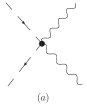
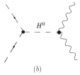
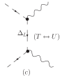
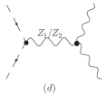
Figure 1: All possible Feynman diagrams for the annihilation processes $\delta_{L}^{0}{\delta_{L}^{0}}^{*}\rightarrow VV$, where $\Delta_{L}$ may be $\delta_{L}^{0/0*}$ or $\delta_{L}^{\pm}$, and $H^{0}$ denotes $h^{0}$, $H_{1}^{0}$ and $H_{2}^{0}$.

In Fig. 1, we show all possible Feynman diagrams for the process $\delta_{L}^{0}{\delta_{L}^{0}}^{*}\rightarrow VV$. There are three kinds of Feynman diagrams Fig. 1a, 1b and 1c for the final states $Z_{1}Z_{1}$. Obviously, the amplitude of Fig. 1b is suppressed by a factor of $\kappa/\sqrt{s}$ compared with the first one. Thus we only consider the contribution from Fig. 1a and 1c. The total annihilation cross section is found to be

$$\omega_{Z_{1}Z_{1}}\approx\frac{2e^{4}\csc^{4}2\theta_{W}}{\pi}\left[1+\frac{4m^{2}}{s}-\frac{8m^{2}(s-2m^{2})}{s^{2}}y(x_{1})\right]$$ (24)

where the function $y(x_{1})$ is defined by $y(x_{1})\equiv{\rm arctanh}(x_{1})/x_{1}$ and $x_{1}=\sqrt{1-4m^{2}/s}$. Then, we can derive $(m\sigma_{0})_{Z_{1}Z_{1}}\leq 2.1\times 10^{-5}\;{\rm GeV}^{-1}$ for $m\geq 500$ GeV. It is obvious that this result is not so large as to satisfy the requirement of Eq.(20).

According to the $Z_{1}Z_{1}$ experience, we also calculate the other processes. The corresponding cross sections are given by

$$\omega_{W_{1}W_{1}} \approx \frac{e^{4}}{32\pi\sin^{4}\theta_{W}}\left[3+\frac{28m^{2}}{s}-32\frac{m^{2}}{s}y(x_{1})\right]\;;$$ (25)

$$\omega_{W_{2}W_{2}} \approx \frac{e^{4}}{128\pi\sin^{4}\theta_{W}}\left(1-\frac{4m^{2}_{W_{2}}}{s}\right)^{1/2}\bigg{[}\frac{4}{3}\frac{\sin^{4}\theta_{W}}{\cos^{2}2\theta_{W}}\frac{(s-4m^{2})(s-4m^{2}_{W_{2}})}{(s-m^{2}_{Z_{2}})^{2}}$$ (26)

$$\times \left(1+\frac{20m^{2}_{W_{2}}}{s}+12\frac{m^{4}_{W_{2}}}{s^{2}}\right)+\left(\frac{\rho_{3}v_{R}^{2}}{m^{2}_{W_{2}}}\right)^{2}\frac{s^{2}-4m^{2}_{W_{2}}s+12m^{4}_{W_{2}}}{(s-m^{2}_{H_{2}^{0}})^{2}}\bigg{]};$$

$$\omega_{Z_{1}Z_{2}} \approx \frac{e^{4}\sec^{4}\theta_{W}}{4\pi\cos 2\theta_{W}}\left(1-\frac{m^{2}_{Z_{2}}}{s}\right)$$ (27)

$$\times \frac{s^{2}-3m^{2}_{Z_{2}}s+m^{4}_{Z_{2}}+4m^{2}s-2(s-2m^{2})(4m^{2}-m^{2}_{Z_{2}})y(x_{1})}{(s-m^{2}_{Z_{2}})^{2}}\;;$$

$$\omega_{Z_{2}Z_{2}} \approx \frac{e^{4}\tan^{4}\theta_{W}}{32\pi\cos^{2}2\theta_{W}}\left(1-\frac{4m^{2}_{Z_{2}}}{s}\right)^{1/2}$$ (28)

$$\times \bigg{[}4+\frac{(4m^{2}-m^{2}_{Z_{2}})^{2}}{m^{2}s-4m^{2}m^{2}_{Z_{2}}+m^{4}_{Z_{2}}}-4x_{\rho}[2+\frac{8m^{2}-s-2m^{2}_{Z_{2}}}{s-2m^{2}_{Z_{2}}}y(x_{2})]$$

$$- \frac{16(2m^{2}-m^{2}_{Z_{2}})s-4m^{2}(16m^{2}-7m^{2}_{Z_{2}})}{(s-2m^{2}_{Z_{2}})^{2}}y(x_{2})+(6-\frac{2s}{m^{2}_{Z_{2}}}+\frac{s^{2}}{2m^{4}_{Z_{2}}})x^{2}_{\rho}\bigg{]},$$

where $x_{\rho}=(\cot^{4}\theta_{w}\rho_{3}v_{R}^{2})/(s-m^{2}_{H_{2}^{0}})$ and $x_{2}\equiv\sqrt{(s-4m^{2})(s-4m_{Z_{2}}^{2})}/(s-2m_{Z_{2}}^{2})$. These cross sections have the same order as the $Z_{1}Z_{1}$ case. However, the thermally averaged annihilation cross sections of these processes (except for $W_{1}W_{1}$) are far less than the $Z_{1}Z_{1}$ case with $m=500$ GeV. Therefore, we don’t analyze these processes in detail.

V.3 $\delta_{L}^{0}{\delta_{L}^{0}}^{*}\rightarrow HH/VH$

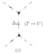
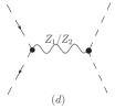
Figure 2: All possible Feynman diagrams for the annihilation processes $\delta_{L}^{0}{\delta_{L}^{0}}^{*}\rightarrow HH$.

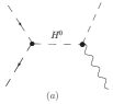
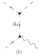
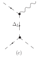
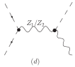
Figure 3: All possible Feynman diagrams are shown for the annihilation processes $\delta_{L}^{0}{\delta_{L}^{0}}^{*}\rightarrow VH$. The first diagram only appears in the process $\delta_{L}^{0}\delta_{L}^{0*}\rightarrow VA_{1}^{0}$

Let’s now focus on the processes $\delta_{L}^{0}{\delta_{L}^{0}}^{*}\rightarrow HH/VH$. The relevant Feynman diagrams for $HH$ and $HV$ are shown in Fig. 2 and Fig. 3, respectively. Since the dimensional scalar trilinear couplings enter extensively into the above two annihilation processes, the electroweak scale coupling $\alpha_{1}\kappa$ in $\delta_{L}^{0}{\delta_{L}^{0}}^{*}h^{0}$ and the right-handed scale coupling $\rho_{3}v_{R}$ in $\delta_{L}^{0}{\delta_{L}^{0}}^{*}H_{2}^{0}$ would make big difference in the $\delta_{L}^{0}{\delta_{L}^{0}}^{*}\rightarrow HV$ processes according to our current parameter setting. Considering the complexity of this model, we only calculate the annihilation cross sections up to leading order (LO) by omitting the next to leading order (NLO) contributions in terms of the following three suppressing factors: (1) small VEV ratio $\kappa/v_{R}$ and $\kappa/\sqrt{s}$ due to the big hierarchy in symmetry breaking scale of the LR model. Since we have made the approximation $\kappa^{2}/v_{R}^{2}\simeq 0$ thus here it is of course a reasonable power counting rule to pick out the LO processes against the NLO ones; (2) gauge coupling suppression $e^{2}$; (3) $p$-wave factor $1-4m^{2}/s$ due to large suppression in the integration of initial energy of dark matter pair.

Process	Amplitude	Order	Process	Amplitude	Order
$h^{0}h^{0}$	$i\alpha_{1}\left(1-\frac{\rho_{3}v_{R}^{2}}{s-2\rho_{1}v_{R}^{2}}\right)$	1	$h^{0}Z_{1}$	$4ie\alpha_{1}\csc 2\theta_{W}\kappa P_{TU}$	$\frac{e^{2}}{x_{f}}\frac{\kappa^{2}}{s}$
$h^{0}H_{1}^{0}$	$2i\alpha_{2}\left(1-\frac{\rho_{3}v_{R}^{2}}{s-2\rho_{1}v_{R}^{2}}\right)$	1	$h^{0}Z_{2}^{0}$	$2ie\alpha_{1}\frac{t_{W}}{\sqrt{c_{2W}}}\kappa P_{TU}$	$\frac{e^{2}}{x_{f}}\frac{\kappa^{2}}{s}$
$H_{1}^{0}H_{1}^{0}$	$i(\alpha_{1}+\alpha_{3})\left(1-\frac{\rho_{3}v_{R}^{2}}{s-2\rho_{1}v_{R}^{2}}\right)$	1	$H_{1}^{0}Z_{1}$	$8ie\alpha_{2}\csc_{2W}\kappa P_{TU}$	$\frac{e^{2}}{x_{f}}\frac{\kappa^{2}}{s}$
$A_{1}^{0}A_{1}^{0}$	$i(\alpha_{1}+\alpha_{3})\left(1-\frac{\rho_{3}v_{R}^{2}}{s-2\rho_{1}v_{R}^{2}}\right)$	1	$H_{1}^{0}Z_{2}$	$4ie\alpha_{2}\frac{t_{W}}{\sqrt{c_{2W}}}\kappa P_{TU}$	$\frac{e^{2}}{x_{f}}\frac{\kappa^{2}}{s}$
$A_{1}^{0}H_{1}^{0}$	$et_{W}\left[c_{2W}P_{Z_{1}}-t_{W}P_{Z_{2}}/2\right]$	$\frac{e^{2}}{x_{f}}$	$A_{1}^{0}Z_{1}$	$4ie\alpha_{2}\csc_{2W}\kappa P^{H}_{43}$	$1$
$H_{2}^{0}H_{2}^{0}$	$i\rho_{3}\left(2-\frac{6\rho_{1}v_{R}^{2}}{s-2\rho_{1}v_{R}^{2}}-\frac{\rho_{3}v_{R}^{2}}{t-m^{2}}-\frac{\rho_{3}v_{R}^{2}}{u-m^{2}}\right)$	1	$A_{1}^{0}Z_{2}$	$-4ie\alpha_{2}\csc_{2W}\sqrt{c_{2W}}\kappa P^{H}_{43}$	$(\frac{\kappa}{v_{R}})^{2}$
$h^{0}H_{2}^{0}$	$-i\rho_{3}\alpha_{1}\kappa v_{R}\left(\frac{1}{s-2\rho_{1}v_{R}^{2}}+\frac{1}{t-m^{2}}+\frac{1}{u-m^{2}}\right)$	$(\frac{\kappa}{v_{R}})^{2}$	$H_{2}^{0}Z_{1}$	$4ie\rho_{3}\csc_{2W}v_{R}P_{TU}$	$\frac{e^{2}}{x_{f}}$
$H_{1}^{0}H_{2}^{0}$	$-2i\rho_{3}\alpha_{2}\kappa v_{R}\left(\frac{1}{s-2\rho_{1}v_{R}^{2}}+\frac{1}{t-m^{2}}+\frac{1}{u-m^{2}}\right)$	$(\frac{\kappa}{v_{R}})^{2}$	$H_{2}^{0}Z_{2}$	$2ie\rho_{3}\frac{t_{W}}{\sqrt{c_{2W}}}v_{R}P_{TU}$	$\frac{e^{2}}{x_{f}}$
$H_{1}^{+}H_{1}^{-}$	$i\alpha_{1}\left[1-(1+\frac{\alpha_{3}}{\alpha_{1}})\frac{\rho_{3}v_{R}^{2}}{s-2\rho_{1}v_{R}^{2}}\right]$	1	$H_{1}^{+}W_{1}^{-}$	$-2ie\alpha_{2}\csc_{2W}\kappa P^{H}_{43}$	1
$\delta_{R}^{++}\delta_{R}^{--}$	$i\rho_{3}\left[1-\frac{2(\rho_{1}+2\rho_{2})v_{R}^{2}}{s-2\rho_{1}v_{R}^{2}}-\frac{\rho_{4}}{\rho_{3}}\frac{8\rho_{4}v_{R}^{2}}{t-m^{2}}\right]$	1	$H_{1}^{+}W_{2}^{-}$	$-2ie\alpha_{2}\csc_{2W}\kappa P^{h}_{43}$	$(\frac{\kappa}{v_{R}})^{2}$

Table 2: The amplitude for $HH/HV$ final states, where $c_{W}=\cos\theta_{W}$, $t_{W}=\tan\theta_{W}$, etc. We also estimate the order of corresponding annihilation cross sections.

In this subsection, we apply the above three suppressing factors to make an explicit demonstration of the LO processes, then give the convincing dark matter annihilation cross sections. The LO amplitude for each possible annihilation process is listed in Table 2. The notations are as follows: $p_{1,2}$ denotes the momentum of the dark matter pair, while $p_{3,4}$ is the momentum of the final states, $\epsilon$ is the polar vector of gauge boson:

$$P_{Z_{1,2}} = \frac{(p_{1}-p_{2})\cdot(p_{4}-p_{3})}{s-m^{2}_{Z_{1,2}}};\hskip 11.38092ptP^{h,H}_{43}=\frac{p_{4}\cdot\epsilon_{(}p_{3})}{s-m^{2}_{h^{0},H_{1}^{0}}};\hskip 11.38092ptP_{TU}=\frac{p_{2}\cdot\epsilon(p_{3})}{t-m^{2}}-\frac{p_{1}\cdot\epsilon(p_{3})}{u-m^{2}}.$$ (29)

Here we only consider the cross sections with amplitude order 1. In terms of Table 2, nine LO annihilation cross sections are listed in Table 3, where $A=1-\frac{2(\rho_{1}+2\rho_{2})}{s-2\rho_{1}v_{R}^{2}}$ and $B=\frac{32\rho_{4}^{2}}{\rho_{3}}\frac{v_{R}^{2}}{s-2m_{\delta_{R}^{\pm\pm}}^{2}}y(x_{3})+\frac{64\rho_{4}^{4}}{\rho_{3}^{2}}\frac{v_{R}^{4}}{sm^{2}-4m^{2}m^{2}_{\delta_{R}^{\pm\pm}}+m^{4}_{\delta_{R}^{\pm\pm}}}$ with $x_{3}=\sqrt{(s-4m^{2})(s-4m^{2}_{\delta_{R}^{\pm\pm}})}/(s-2m^{2}_{\delta_{R}^{\pm\pm}})$; $a=2-\frac{3m^{2}_{H_{2}^{0}}}{s-m^{2}_{H_{2}^{0}}},b=4m^{2}+m^{2}_{H_{2}^{0}},c=s-2m^{2}_{H_{2}^{0}},d=\sqrt{sm^{2}-4m^{2}m^{2}_{H_{2}^{0}}+m^{4}_{H_{2}^{0}}}$ and $x_{4}=\sqrt{(s-4m^{2})(s-4m^{2}_{H_{2}^{0}})}/(s-2m^{2}_{H_{2}^{0}})$. We find that these processes fail to provide enough large cross sections. For $\delta_{L}^{0}{\delta_{L}^{0}}^{*}\rightarrow A_{1}^{0}Z_{1}$ and $H_{1}^{\pm}W_{1}^{\mp}$, one can easily obtain $m\sigma_{0}\lesssim\alpha_{2}^{2}/(16\pi m)$, which is far less than the required lower bound $0.13\;{\rm GeV}^{-1}$. Since the other processes have the similar forms, we take the process $\delta_{L}^{0}{\delta_{L}^{0}}^{*}\rightarrow h^{0}H_{1}^{0}$ as an example to illustrate the main features of this kind of processes. One can immediately derive

$$(m\sigma_{0})_{h^{0}H_{1}^{0}}=\frac{\alpha_{2}^{2}}{8\pi v_{R}}\sqrt{\frac{1}{\varepsilon\rho_{1}}-\frac{1}{4(\varepsilon\rho_{1})^{2}}}\left(\frac{\varepsilon-2}{2\varepsilon-1}\right)^{2}\;,$$ (30)

where we have used $\alpha_{3}=2$. It is obvious that the maximum value can be obtained when $\varepsilon\rho_{1}=0.5$. Varying $\varepsilon$, we may derive $(m\sigma_{0})_{h^{0}H_{1}^{0}}\leq 3.5\times 10^{-4}\;{\rm GeV}^{-1}$ for $\alpha_{2}=2$. Therefore, we don’t discuss this class of processes in detail.

Process	$4E_{1}E_{2}\sigma v$	Process	$4E_{1}E_{2}\sigma v$
$h^{0}h^{0}$	$\frac{\alpha_{1}^{2}}{16\pi}(1-\frac{\rho_{3}v_{R}^{2}}{s-2\rho_{1}v_{R}^{2}})^{2}$	$H_{1}^{+}H_{1}^{-}$	$\frac{\alpha_{1}^{2}}{8\pi}\left[1-(1+\frac{\alpha_{3}}{\alpha_{1}})\frac{\rho_{3}v_{R}^{2}}{s-2\rho_{1}v_{R}^{2}}\right]^{2}$
$h^{0}H_{1}^{0}$	$\frac{\alpha_{2}^{2}}{2\pi}(1-\frac{m^{2}_{H_{1}^{0}}}{s})^{1/2}(1-\frac{\rho_{3}v_{R}^{2}}{s-2\rho_{1}v_{R}^{2}})^{2}$	$\delta_{R}^{++}\delta_{R}^{--}$	$\frac{\rho_{3}^{2}}{8\pi}(1-\frac{4m^{2}_{\delta_{R}^{\pm\pm}}}{s})^{1/2}(A^{2}+B)$
$H_{1}^{0}H_{1}^{0}$	$\frac{(\alpha_{1}+\alpha_{3})^{2}}{16\pi}(1-\frac{4m^{2}_{H_{1}^{0}}}{s})^{1/2}(1-\frac{\rho_{3}v_{R}^{2}}{s-2\rho_{1}v_{R}^{2}})^{2}$	$A_{1}^{0}Z_{1}$	$\frac{\alpha_{2}^{2}}{4\pi}(1-\frac{m^{2}_{A_{1}^{0}}}{s})^{5/2}$
$A_{1}^{0}A_{1}^{0}$	$\frac{(\alpha_{1}+\alpha_{3})^{2}}{16\pi}(1-\frac{4m^{2}_{H_{1}^{0}}}{s})^{1/2}(1-\frac{\rho_{3}v_{R}^{2}}{s-2\rho_{1}v_{R}^{2}})^{2}$	$H_{1}^{+}W_{1}^{-}$	$\frac{\alpha_{2}^{2}}{4\pi}(1-\frac{m^{2}_{H_{1}^{\pm}}}{s})^{5/2}$
$H_{2}^{0}H_{2}^{0}$	$\frac{\rho_{3}^{2}}{16\pi}\left[a^{2}+\frac{b^{2}}{2d^{2}}+\frac{2b}{c}(2a+\frac{b}{c})y(x_{4})\right]$

Table 3: The annihilation cross sections for the leading order processes.

V.4 The resonance case

As pointed out in the previous discussion, the method of calculating the effective thermally averaged annihilation cross section $\langle\sigma_{eff}v\rangle$ is not valid for the resonance case CO . Here we numerically solve the Boltzmann equation Eq.(15), which can be reexpressed as Gondolo

$$\frac{dY}{dx} = -\frac{x}{H_{x=1}{\bf s}(x)}\gamma_{eff}\left(\frac{Y^{2}}{Y^{2}_{\rm eq}}-1\right)\ ,$$ (31)

where $H_{x=1}$ is the Hubble parameter evaluated at $T=m$ and ${\bf s(x)}$ is the entropy density given by

$$H_{x=1}=\sqrt{\frac{4\pi^{3}g_{\ast}}{45}}\,\frac{m^{2}}{M_{Pl}}\;,\quad{\bf s}(x)=\frac{2\pi^{2}g_{\ast}}{45}\frac{m^{3}}{x^{3}}\;.$$ (32)

$Y\equiv n/{\bf s}$ is the ratio of the total particle number density $n$ to the entropy density ${\bf s}$. The equilibrium number density $Y_{\rm eq}$ reads

$$Y_{\rm eq}(x)=\frac{45}{4\pi^{4}}\frac{g_{eff}}{g_{\ast}}x^{2}K_{2}\left(x\right)\,.$$ (33)

In fact, $\gamma_{eff}$ is the reaction density defined by

$$\gamma_{eff}\equiv n_{eq}^{2}\langle\sigma_{eff}v\rangle=\frac{m^{4}}{64\,\pi^{4}x}\int_{4}^{\infty}\hat{\sigma}_{eff}(z)\,\sqrt{z}\,K_{1}(x\,\sqrt{z})\,dz\,,$$ (34)

with

$$\hat{\sigma}_{eff}=g_{eff}^{2}4E_{1}E_{2}\sigma_{eff}v\sqrt{1-4/z}\;,$$ (35)

where $z=s/m^{2}$, $K_{1}(x)$ and $K_{2}(x)$ are the modified Bessel functions.

$\rho_{1}=1.0$	$n_{\delta_{L}^{0}}$	$\rho_{1}=0.1$	$n_{\delta_{L}^{0}}$
$\alpha_{1}=0.01$	$n_{\delta_{L}^{0}}=6.4\times 10^{-13}$	$\alpha_{1}=0.01$	$n_{\delta_{L}^{0}}=1.6\times 10^{-12}$
$\alpha_{1}=0.1$	$n_{\delta_{L}^{0}}=6.5\times 10^{-13}$	$\alpha_{1}=0.1$	$n_{\delta_{L}^{0}}=1.4\times 10^{-12}$
$\alpha_{1}=1.0$	$n_{\delta_{L}^{0}}=1.1\times 10^{-12}$	$\alpha_{1}=1.0$	$n_{\delta_{L}^{0}}=3.6\times 10^{-12}$
$\alpha_{1}=2.0$	$n_{\delta_{L}^{0}}=2.5\times 10^{-12}$	$\alpha_{1}=2.0$	$n_{\delta_{L}^{0}}=1.2\times 10^{-11}$

Table 4: The relic number density $n_{\delta_{L}^{0}}$ in terms of different $\alpha_{1}$ and $\rho_{1}$ for the $H_{2}^{0}$ case.

In our scenario, the exchanged particles may be $Z_{1}$, $Z_{2}$, $h^{0}$, $H_{1}^{0}$ and $H_{2}^{0}$. It is obvious that the case of exchanging gauge bosons $Z_{1}$ or $Z_{2}$ is a $p$-wave annihilation process. If the exchanged particle is $H_{1}^{0}$, the corresponding cross section will be suppressed by $\kappa^{2}/v_{R}^{2}$. For the $h^{0}$ case, the resonant condition $2m\approx m_{h^{0}}$ implies that the final states must be the Fermi pairs. In addition, the previous analysis indicates that the maximal cross section might be from the $H_{2}^{0}$ exchanging process. Therefore, we study the $h^{0}$ and $H_{2}^{0}$ cases in this subsection.

Firstly we consider the $H_{2}^{0}$ case. Due to the factor $\sqrt{1-4/z}$ in Eq. (35), we take $m^{2}_{H_{2}^{0}}/m^{2}=4.1$ (namely $\varepsilon=0.4878$). At this point, $\gamma_{eff}$ becomes more larger than the $m^{2}_{H_{2}^{0}}/m^{2}=4$ case. Then we take $\rho_{1}=1$ ($\rho_{3}=2.98$). At this moment, $\delta_{L}^{0}$ and ${\delta_{L}^{0}}^{*}$ may annihilate into $h^{0}h^{0}$, $h^{0}H_{1}^{0}$ and $W_{2}W_{2}$. Since $h^{0}h^{0}$ and $h^{0}H_{1}^{0}$ have the similar form, the key quantity is $\alpha_{2}^{2}+\alpha_{1}^{2}/8$ for our calculation. Without loss of generality, one may take different values for $\alpha_{1}$ and require $\alpha_{1}=\alpha_{2}$. The final results for different $\alpha_{1}$ have been shown in Table 4. In addition, we also calculate the $\rho_{1}=0.1$ case, and list the corresponding results in Table 4. If $\rho_{1}=0.1$, the final states have to be two SM Higgs bosons. In views of Table 4, we may find that the $H_{2}^{0}$ case fails to suppress the relic number density of $\delta_{L}^{0}$ and ${\delta_{L}^{0}}^{*}$.

Figure 4: Numerical illustration of the relic number density $n_{\delta_{L}^{0}}$ as a function of $2m/m_{h^{0}}$ near a resonance, where $m_{h^{0}}=120$ GeV has typically been taken. The dashed line denotes the present experimental upper bound on $n_{\delta_{L}^{0}}$.

Now we assume the SM Higgs mass $m_{h^{0}}=120$ GeV in the $h^{0}$ case. Furthermore, one may obtain $m=59.3$ GeV ($\varepsilon\rho_{1}=3.5\times 10^{-5}$) from $m^{2}_{H_{2}^{0}}/m^{2}=4.1$. Because of $m<100$ GeV, the bound in Eq.(14) is not valid. For $m=59.3$ GeV, we take $\sigma_{n}^{exp}\leq 4.6\times 10^{-44}\,{\rm cm^{2}}$ CDMS and derive the corresponding bound

$$n_{\delta_{L}^{0}}\leq 1.1\times 10^{-13}\;.$$ (36)

In this case, $\delta_{L}^{0}$ and ${\delta_{L}^{0}}^{*}$ mainly annihilate into the bottom quark pair. The annihilation cross section is given by

$$(4E_{1}E_{2}\sigma v)_{h^{0}}\simeq\frac{3}{4\pi}\frac{\alpha_{1}^{2}m_{b}^{2}s}{(s-m_{h^{0}}^{2})^{2}+m_{h^{0}}^{2}\Gamma_{h^{0}}^{2}}$$ (37)

where $m_{b}$ is the bottom quark mass and $\Gamma_{h^{0}}\simeq 3m_{h^{0}}m_{b}^{2}/(8\pi\kappa^{2})$ is the decay width of $h^{0}$. One may obtain $n_{\delta_{L}^{0}}=1.2\times 10^{-15}$ for $\alpha_{1}=2$. This wonderful result indicates that our scenario may be consistent with the direct dark matter search bound. To illustrate, we plot the relic number density $n_{\delta_{L}^{0}}$ versus the dark matter mass $m$ in Fig. 4, where all annihilation channels have been considered. Using the results from CERN LEP-II, Datta and Raychaudhuri have derived $m\geq 55.4$ GeV Datta . To show the $h^{0}$ resonance region, we choose 48 GeV $\leq m\leq 72$ GeV ($0.8\leq 2m/m_{h^{0}}\leq 1.2$) in Fig. 4. The peak around $2m/m_{h^{0}}=0.83$ in Fig. 4 is due to the competition between $h^{0}$ and $Z_{1}$ resonances. For $m_{h^{0}}=120$ GeV, we find that $56{\rm GeV}\lesssim m\lesssim 60{\rm GeV}$ can satisfy the requirement $n_{\delta_{L}^{0}}\leq 1.1\times 10^{-13}$. At this moment, one may obtain $\Omega_{\delta_{L}^{0}}h^{2}\lesssim 6.3\times 10^{-7}$, which is far less than the total dark matter density $\Omega_{DM}h^{2}=0.111\pm 0.006$ PDG .

VI Two Higgs bi-doublets model

Motivated by the general two Higgs doublet model as a model for spontaneous CP violation, one may simply extend the one Higgs bi-doublet LR model to a two Higgs bi-doublets LR model with spontaneous P and CP violation Wu . Besides one left-handed Higgs triplet $\Delta_{L}$ (3,1,2) and one right-handed Higgs triplet $\Delta_{R}$ (1,3,2), this model consists of two Higgs bi-doublets $\phi$ (2,2,0) and $\chi$ (2,2,0), which can be written as

$$\phi=\left(\matrix{\phi_{1}^{0}&\phi_{1}^{+}\cr\phi_{2}^{-}&\phi_{2}^{0}\cr}\right);\;\chi=\left(\matrix{\chi_{1}^{0}&\chi_{1}^{+}\cr\chi_{2}^{-}&\chi_{2}^{0}\cr}\right)\;.$$ (38)

The most general Yukawa interaction for quarks is given by

$$-{\cal L}_{Y}=\overline{Q_{L}}\left(Y_{q}\phi+\tilde{Y}_{q}\tilde{\phi}+F_{q}\chi+\tilde{F}_{q}\tilde{\chi}\right)Q_{R}\;,$$ (39)

where $Q_{L,R}=(u_{L,R},d_{L,R})^{T}$. Parity P symmetry requires $Y_{q}$, $\tilde{Y}_{q}$, $F_{q}$ and $\tilde{F}_{q}$ are hermitian matrices. When both P and CP are required to be broken down spontaneously, all the Yukawa couplings matrices are real symmetric. After the spontaneous symmetry breaking, two Higgs bi-doublets can have the following vacuum expectation values

$$\langle\phi\rangle=\left(\matrix{\kappa_{1}/\sqrt{2}&0\cr 0&\kappa_{2}/\sqrt{2}\cr}\right);\;\langle\chi\rangle=\left(\matrix{w_{1}/\sqrt{2}&0\cr 0&w_{2}/\sqrt{2}\cr}\right)\;,$$ (40)

where $\kappa_{1}$, $\kappa_{2}$, $w_{1}$ and $w_{2}$ are in general complex. Then we may obtain the following quark mass matrices

$$M_{u} = \frac{1}{\sqrt{2}}(Y_{q}\kappa_{1}+\tilde{Y}_{q}\kappa_{2}+F_{q}w_{1}+\tilde{F}_{q}w_{2})\;;$$

$$M_{d} = \frac{1}{\sqrt{2}}(Y_{q}\kappa_{2}+\tilde{Y}_{q}\kappa_{1}+F_{q}w_{2}+\tilde{F}_{q}w_{1})\;.$$ (41)

In the two Higgs bi-doublets model, the stringent constraints from the low energy phenomenology can be significantly relaxed. In Ref. Wu , the authors calculate the constraints from neural $K$ meson mass difference $\Delta m_{K}$ and demonstrate that a right-handed gauge boson $W_{2}$ contribution in box-diagrams with mass around 600 GeV is allowed due to a cancelation caused by a light charged Higgs boson with a mass range $150-300$ GeV. Therefore, we take $v_{R}\approx 2$ TeV instead of the previous $v_{R}=10$ TeV for this section. It is worthwhile to stress that our previous estimation is still right for this case except for the process $\delta_{L}^{0}{\delta_{L}^{0}}^{*}\rightarrow h^{0}H_{1}^{0}$. $(m\sigma_{0})_{h^{0}H_{1}^{0}}$ in Eq.(30) will be about 5 times larger than that in the $v_{R}=10$ TeV case, which does not affect our conclusion.

Since there are two Higgs bi-doublets, we can give more dark matter annihilation processes for $\delta_{L}^{0}{\delta_{L}^{0}}^{*}\rightarrow HH$ and $\delta_{L}^{0}{\delta_{L}^{0}}^{*}\rightarrow VH$. In this model, one may obtain three light neutral Higgs bosons and a pair of light charged Higgs bosons Wang . The other Higgs bosons’ masses are related to $v_{R}$. Although the annihilation cross section might be doubled or even increased by several times, it is still at least 10 times less than the direct dark matter search bound.

An significant advantage of the two Higgs bi-doublets model is that the Yukawa couplings may become very large. In view of Eq. (41), one can explicitly understand this feature. For example, we require the couplings $Y_{q}$ and $\tilde{Y}_{q}$ are very large when $w_{1}\gg\kappa_{1}\gg\kappa_{2}\approx w_{2}$. Then one may obtain more larger annihilation cross section for the $\delta_{L}^{0}{\delta_{L}^{0}}^{*}\rightarrow f\bar{f}$ process than Eq.(23). For illustration, we take the maximal annihilation cross section for each quark pair final states

$$4E_{1}E_{2}\sigma v\sim\frac{3}{8\pi}\frac{(\alpha_{i}Y_{q}w_{1})^{2}s}{(s-m_{h}^{2})^{2}}\;,$$ (42)

where $m_{h}$ denotes the mass of a light Higgs boson which comes from $\phi_{1}^{0}$. For $\alpha_{i}=1$, $w_{1}\approx 246$ GeV and $m=100$ GeV, $Y_{q}\gtrsim 4.3$ can be obtained from Eq.(20) when we take $2m/m_{h}=0.8$ and consider all quark final states but top quark. At this moment, we must consider the light Higgs $h$ contribution to the direct dark matter detection experiments. The WIMP-nucleon cross section by exchanging $h$ is given by

$$\sigma_{n}=\frac{M^{2}(n)}{2\pi}\left(\frac{\alpha_{i}}{mm_{h}^{2}}\right)^{2}f^{2}M_{n}^{2}$$ (43)

where $f\sim 0.02Y_{q}w_{1}/m_{u}$ DM . Using the above parameter setting, we may derive $\sigma_{n}\gtrsim 6.1\times 10^{-35}\;{\rm cm}^{2}$, which is far more than the $Z_{1}$ exchanging case of Eq.(13). The more larger $Y_{q}$ is, the more larger $\sigma_{n}$ is. Therefore, we can not give the desired relic number density through increasing the Yukawa couplings.

Now we focus on the resonance case. For the $H_{2}^{0}$ exchanging case, the results in Table 4 can be increased by about 5 times because of $v_{R}\approx 2$ TeV. On the other hand, more final states would generally increase the partial width $\Gamma_{H_{2}^{0}\rightarrow HH}$. Namely the case of more final states is equivalent to enhancing $\alpha_{1}$, which does no good for larger annihilation cross section as shown in Table 4. For the $h^{0}$ case, we may obtain the same conclusion as the one Higgs bi-doublet case.

VII Summary and Comments

In the Left-Right symmetric model with one Higgs bi-doublet, we have demonstrated that the cold dark matter constraints should be considered in a specific scenario in which the so-called VEV-seesaw problem can be naturally solved. In such a scenario, we find that $\delta_{L}^{0}$ and ${\delta_{L}^{0}}^{*}$ are two degenerate and stable particles. To avoid the conflict with the direct dark matter detection experiments, we obtain the relic number density $n_{\delta_{L}^{0}}\leq 4.8\times 10^{-14}$, which implies that the two particles can’t dominate all the dark matter. Subsequently, the lower bounds $m\sigma_{0}\geq 0.13\;{\rm GeV}^{-1}$ and $m\sigma_{0}\geq 9.8\;{\rm GeV}^{-1}$ have been derived for the $s$-wave annihilation and the $p$-wave annihilation, respectively. In this paper, we examine whether our scenario can provide very large annihilation cross sections so as to give the desired relic abundance. We analyze in detail four classes of annihilation processes: $\delta_{L}^{0}{\delta_{L}^{0}}^{*}\rightarrow f\bar{f}$, $\delta_{L}^{0}{\delta_{L}^{0}}^{*}\rightarrow VV$, $\delta_{L}^{0}{\delta_{L}^{0}}^{*}\rightarrow HH$ and $\delta_{L}^{0}{\delta_{L}^{0}}^{*}\rightarrow VH$. However, our analysis shows that this scenario fails to suppress the relic number density of $\delta_{L}^{0}$ and ${\delta_{L}^{0}}^{*}$ except for the resonance case . For the $h^{0}$ resonance case, we obtain $\Omega_{\delta_{L}^{0}}h^{2}\lesssim 6.3\times 10^{-7}$, which is far less than the total dark matter density $\Omega_{DM}h^{2}=0.111\pm 0.006$. Finally, we discuss the two Higgs bi-doublet model from the following three aspects: (1) $v_{R}\approx 2$ TeV; (2) more final states; (3) large Yukawa couplings. It turns out that our previous conclusions can be generalized to the two Higgs bi-doublet model.

In recent years, several authors have shown that it is far from natural for the minimal LR model to generate spontaneous CP violation with natural-sized Higgs potential parameters Mohapatra ; VEV ; Barenboim . It is of importance for us to comment on some more general LR models with one Higgs bi-doublet Langacker ; Bernabeu ; Pos ; Frere ; Kie ; Ji . The differences mainly come from the complexity of Higgs potential parameter $\alpha_{2}$ and Yukawa couplings. We stress that our conclusion in Sec V could be generalized to these more general cases without any dramatic alternation because the gauge and Higgs sectors are basically the same.

Appendix A scalar and scalar-gauge trilinear and quartic Couplings

We intend to calculate the cross section to the leading order for each process of dark matter annihilation. We first work in the framework of simple left-right symmetric model with one Higgs bi-doublet and one pair of LR triplets. To simplify our calculation, we take the decoupling limit in which $\kappa^{2}/v_{R}^{2}\simeq 0$ where $\kappa^{2}=|\kappa_{1}|^{2}+|\kappa_{2}|^{2}$ denotes the EWSB scale. The VEVs of the Higgs bi-doublet are required to satisfy the low energy phenomenology constraint $\kappa_{2}/\kappa_{1}\leq m_{b}/m_{t}$, which may produce correct quark masses, small quark mixing angles and the suppression of flavor-changing neutral currents Ecker ; J.-M. Frere ; M.Raidal ; Ball . For simplicity, we take $\kappa_{2}\simeq 0$ which is a reasonable approximation at the leading order since $\kappa_{2}/\kappa_{1}$ is now around $10^{-2}$. Actually the limit $\kappa_{2}\rightarrow 0$ brings additional advantage that the vacuum CP phase $\theta_{2}$ could be taken zero safely without hampering the estimation. These approximations could largely simplify our calculation.

Interaction	Coupling / $v_{R}$	Interaction	Coupling / $\kappa$	Interaction	Coupling
$\delta_{L}^{0}{\delta_{L}^{0}}^{*}H_{2}^{0}$	$\rho_{3}$	$\delta_{L}^{0}{\delta_{L}^{0}}^{*}h^{0}$	$\alpha_{1}$	$\delta_{L}^{0}{\delta_{L}^{0}}^{*}h^{0}h^{0}$	$\alpha_{1}$
$\delta_{L}^{0}\delta_{L}^{--}\delta_{R}^{++}$	$2\sqrt{2}\rho_{4}$	$\delta_{L}^{0}{\delta_{L}^{0}}^{*}H_{1}^{0}$	$2\alpha_{2}$	$\delta_{L}^{0}{\delta_{L}^{0}}^{*}h^{0}H_{1}^{0}$	$2\alpha_{2}$
$H_{2}^{0}h^{0}h^{0}$	$\alpha_{1}$	$h^{0}h^{0}h^{0}$	$6\lambda_{1}$	$\delta_{L}^{0}{\delta_{L}^{0}}^{*}H_{1}^{0}H_{1}^{0}$	$\alpha_{1}+\alpha_{3}$
$H_{2}^{0}H_{1}^{0}h^{0}$	$2\alpha_{2}$	$H_{1}^{0}h^{0}h^{0}$	$6\lambda_{4}$	$\delta_{L}^{0}{\delta_{L}^{0}}^{*}A_{1}^{0}A_{1}^{0}$	$\alpha_{1}+\alpha_{3}$
$H_{2}^{0}H_{1}^{0}H_{1}^{0}$	$\alpha_{1}+\alpha_{3}$	$H_{1}^{0}H_{1}^{0}h^{0}$	$2\tilde{\lambda}$	$\delta_{L}^{0}{\delta_{L}^{0}}^{*}H_{1}^{+}H_{1}^{-}$	$\alpha_{1}$
$H_{2}^{0}A_{1}^{0}A_{1}^{0}$	$\alpha_{1}+\alpha_{3}$	$H_{1}^{0}H_{1}^{0}H_{1}^{0}$	$6\lambda_{4}$	$\delta_{L}^{0}{\delta_{L}^{0}}^{*}H_{2}^{0}H_{2}^{0}$	$2\rho_{3}$
$H_{2}^{0}H_{1}^{+}H_{1}^{-}$	$\alpha_{1}+\alpha_{3}$	$H_{1}^{0}A_{1}^{0}H_{1}^{0}$	$2\lambda_{4}$	$\delta_{L}^{0}{\delta_{L}^{0}}^{*}\delta_{R}^{++}\delta_{R}^{--}$	$\rho_{3}$
$H_{2}^{0}H_{2}^{0}H_{2}^{0}$	$6\rho_{1}$	$h^{0}A_{1}^{0}A_{1}^{0}$	$2\tilde{\lambda}^{\prime}$
$H_{2}^{0}\delta_{R}^{++}\delta_{R}^{--}$	$2(\rho_{1}+2\rho_{2})$	$H_{2}^{0}H_{2}^{0}h^{0}$	$\alpha_{1}$
		$H_{2}^{0}H_{2}^{0}H_{1}^{0}$	$2\alpha_{2}$

Table 5: The relevant trilinear and quartic scalar couplings, where the dimensional trilinear couplings with different scales $v_{R}$ and $\kappa$ are separated shown separately in two columns. $\tilde{\lambda}=\lambda_{1}+4\lambda_{2}+2\lambda_{3}$ and $\tilde{\lambda}^{\prime}=\lambda_{1}-4\lambda_{2}+2\lambda_{3}$

The relevant scalar trilinear couplings and quartic couplings under the unitary gauge are shown in Table 5. Here we write out the scalar-gauge interactions:

$$\mathcal{L}_{\delta_{L}^{0}{\delta_{L}^{0}}^{*}VV} = \delta_{L}^{0}{\delta_{L}^{0}}^{*}(gW_{3L}-g^{\prime}B)^{2}+g^{2}\delta_{L}^{0}{\delta_{L}^{0}}^{*}W_{L}^{+}W_{L}^{-};$$ (44)

$$\mathcal{L}_{\delta_{L}^{0}\delta_{L}V} = -ig(\delta_{L}^{0}\partial\delta_{L}^{-}-\delta_{L}^{-}\partial\delta_{L}^{0})W_{L}^{+}+i\delta_{0}\partial{\delta_{L}^{0}}^{*}(gW_{3L}-g^{\prime}B)+h.c.;$$ (45)

$$\mathcal{L}_{HVV} = g^{2}v_{R}\left\{H_{2}^{0}[(gW_{3R}-g^{\prime}B)(gW_{3R}-g^{\prime}B)+W_{R}^{+}W_{R}^{-}]+(-\frac{1}{\sqrt{2}}\delta_{R}^{--}W_{R}^{+}W_{R}^{+}+h.c.)\right\}$$ (46)

$$+ g^{2}k\bigg{\{}\frac{1}{2}H_{1}^{-}(W_{3R}W_{L}^{+}-W_{3L}W_{R}^{+})-\frac{1}{2}(H_{1}^{0}+iA_{1}^{0})W_{L}^{-}W_{R}^{+}+h.c.$$

$$+ \frac{1}{4}h^{0}[(W_{3L}-W_{3R})(W_{3L}-W_{3R})+2(W_{L}^{+}W_{L}^{-}+W_{R}^{+}W_{R}^{-})]\bigg{\}};$$

$$\mathcal{L}_{HHV} = \frac{ig}{2}H_{1}^{-}\partial H_{1}^{+}(W_{3L}+W_{3R})-i\delta_{R}^{++}\partial\delta_{R}^{--}(gW_{3R}+g^{\prime}B)-ig(\delta_{R}^{--}\partial\delta_{R}^{+}-\delta_{R}^{+}\partial\delta_{R}^{--})W_{R}^{+}$$ (47)

$$+ \frac{ig}{2}\left[(H_{1}^{-}\partial H_{1}^{0}-H_{1}^{0}\partial H_{1}^{-})W_{L}^{+}+(h^{0}\partial H_{1}^{-}-H_{1}^{-}\partial h^{0})W_{R}^{+}\right]$$

$$+ \frac{g}{2}\left[(A_{1}^{0}\partial H_{1}^{-}-H_{1}^{-}\partial A_{1}^{0})W_{R}^{+}+h.c.\right.$$

$$+ \left.(H_{1}^{0}\partial A_{1}^{0}-A_{1}^{0}\partial H_{1}^{0})(W_{3L}-W_{3R})\right],$$

where the connection between weak eigenstates $(W_{3L},W_{3R},B)$ and physical states $(Z_{1},Z_{2},A)$ are demonstrated by the following orthogonal transformation at the leading order:

$$\left(\begin{array}[]{c}W_{3L}\\ W_{3R}\\ B\\ \end{array}\right) = \left(\begin{array}[]{ccc}c_{W}&0&s_{W}\\ -s_{W}t_{W}&\sqrt{c_{2W}}\sec_{W}&s_{W}\\ -\sqrt{c_{2W}}t_{W}&-t_{W}&\sqrt{c_{2W}}\\ \end{array}\right)\left(\begin{array}[]{c}Z_{1}\\ Z_{2}\\ A\\ \end{array}\right)\;.$$ (57)

The $SU(2)_{L,R}$ gauge coupling $g$ and $U(1)_{B-L}$ coupling $g^{\prime}$ are related to $U(1)_{EM}$ gauge coupling $e$:

$$g=\frac{e}{\sin\theta_{W}},\hskip 28.45274ptg^{\prime}=\frac{e}{\sqrt{\cos 2\theta_{W}}}\;.$$ (58)

Here our conventions are the same as those in Ref. DUKA .

References

(1) J. C. Pati and A. Salam, Phys. Rev. D 10, 275 (1974); R. N.
Mohapatra and J. C. Pati, Phys. Rev. D 11, 566 (1975); G.
Senjanovic and R. N. Mohapatra, Phys. Rev. D 12, 1502 (1975).
(2) T. D. Lee, Phys. Rev. D 8, 1226 (1973); Phys. Rep. 9, 143 (1974).
(3) A. Masiero, R. N. Mohapatra and R. D. Peccei, Nucl. Phys. B192, 66 (1981). J. Basecq,
J. Liu, J. Milutinovic and L. Wolfenstein, Nucl. Phys. B272,
145 (1986).
(4) N. G. Deshpande, J. F. Gunion, B. Kayser and F.
Olness, Phys. Rev. D 44, 837 (1991).
(5)G. Barenboim, M. Gorbahn, U. Nierste and M. Raidal, Phys. Rev. D 65, 095003
(2002); Y. Rodriguez and C. Quimbay, Nucl. Phys. B637, 219
(2002).
(6) P. Langacker and S. U. Sankar, Phys. Rev. D 40, 1569 (1989).
(7)G. Barenboim, J. Bernabeu, J. Prades and M. Raidal, Phys. Rev. D 55, 4213 (1997).
(8) M. E. Pospelov, Phys. Rev. D 56,
259 (1997).
(9) P. Ball, J. M. Frere and J. Matias, Nucl. Phys. B572, 3
(2000).
(10) K. Kiers, M. Assis and A. A. Petrov, Phys. Rev. D 71, 115015
(2005).
(11) Y. Zhang, H. P. An, X. D. Ji and R. N. Mohapatra,
arXiv:0704.1662; Y. Zhang, H. P. An, X. D. Ji and R. N. Mohapatra,
arXiv:0712.4218.
(12) K. Kiers, J. Kolb, J. Lee, A. Soni and G. H. Wu , Phys. Rev. D 66, 095002
(2002).
(13) Y. L. Wu and Y. F. Zhou, arXiv:0709.0042.
(14) P. Minkowski, Phys. Lett. B 67, 421 (1977); T. Yanagida, in
Proceedings of the Workshop on Unified Theory and the Baryon
Number of the Universe, edited by O. Sawada and A. Sugamoto (KEK,
Tsukuba, 1979); M. Gell-Mann, P. Ramond, and R. Slansky, in Supergravity, edited by F. van Nieuwenhuizen and D. Freedman (North
Holland, Amsterdam, 1979); S.L. Glashow, in Quarks and
Leptons, edited by M. Lvy et al. (Plenum, New
York, 1980); R.N Mohapatra and G. Senjanovic, Phys. Rev. Lett. 44, 912 (1980).
(15) For a review, see: G. Jungman, M. Kamionkowski and K.
Griest, Phys. Rept. 267, 195 (1996); G. Bertone, D. Hooper and
J. Silk, Phys. Rept. 405, 279 (2005).
(16) CDMS collaboration, arXiv:0802.3530; Phys. Rev. Lett. 96, 011302
(2006).
(17) XENON collaboration, Phys. Rev. Lett. 100, 021303
(2008).
(18) Particle Data Group, W. M. Yao et al.,
J. Phys. G33, 1 (2006).
(19) O. Khasanov and G. Perez, Phys. Rev. D 65,
053007 (2002).
(20) P. Duka, J. Gluza and M. Zralek, Annals Phys. 280, 336
(2000).
(21) J. D. Lewin and P. F. Smith, Astropart. Phys. 6, 87 (1996).
(22) M. Cirelli, N. Fornengo and A. Strumia, Nucl. Phys. B753, 178
(2006).
(23) R. Barbieri, L. J. Hall and V. S. Rychkov, Phys. Rev. D 74,
015007 (2006); E. M. Dolle and S. F. Su, arXiv:0712.1234.
(24) J. D. Bekenstein, Phys. Rev. D 70, 083509
(2004); C. Skordis, D. F. Mota, P. G. Ferreira and C. Boehm, Phys.
Rev. Lett. 96, 011301 (2006); I. Ferreras, M. Sakellariadou
and M. F. Yusaf, Phys. Rev. Lett. 100, 031302 (2008); X. F.
Wu, B. Famaey, G. Gentile, H. Perets and H. S. Zhao,
arXiv:0803.0977; and references cited therein.
(25) K. Griest and D. Seckel, Phys. Rev. D 43, 3191
(1991).
(26) E. W. Kolb and M. S. Turner, The Early Universe,
Addison-Wesley, Reading, MA, (1990).
(27) M. Srednicki, R. Watkins and K. A. Olive, Nucl. Phys. B310, 693
(1988); P. Gondolo and G. Gelmini, Nucl. Phys. B360, 145
(1991).
(28) J. Edsjo and P. Gondolo, Phys. Rev. D 56,
1879 (1997).
(29) A. Datta and A. Raychaudhuri, Phys. Rev. D 62,
055002 (2000).
(30) Y. J. Huo, L. M. Wang and Y. L. Wu, in preparation.
(31) G. Ecker, W. Grimus, W. Konetschny, Phys. Lett. B 94, 381 (1980);
Nucl. Phys. B177, 489 (1981).
(32) J. M. Frere, J. Galand, et al., Phys. Rev. D 46, 337 (1992).
(33) G. Barenboim, J. Bernabeu, M. Raidal, Nucl. Phys. B478, 527
(1996).