Fast Dynamos in Weakly Ionized Gases

Abstract

The turnover of interstellar gas on $\sim 10^{9}$yr timescales argues for the continuous operation of a galactic dynamo. The conductivity of interstellar gas is so high that the dynamo must be “fast” - i.e. the magnetic field must be amplified at a rate nearly independent of the magnetic diffusivity. Yet, all the fast dynamos so far known - and all direct numerical simulations of interstellar dynamos - yield magnetic power spectra that peak at the resistive scale, while galactic magnetic fields have substantial power on large scales. In this paper we show that in weakly ionized gas the limiting scale may be the ion-neutral decoupling scale, which although still small is many orders of magnitude larger than the resistive scale.

1 Introduction

Despite many theoretical and observational advances, our understanding of galactic magnetic fields is still incomplete. Although there is evidence for magnetic fields in young galaxies (Kulsrud & Zweibel 2008), it is likely that dynamo processes still operate continuously in galaxies today. Perhaps the most compelling argument for ongoing dynamo activity is that the turnover time of interstellar gas due to loss and replacement of material - $\sim$ 10⁹ yr in the case of the Milky Way - is much less than the ages of galaxies. As interstellar gas is added - whether by infall from the IGM or through stellar mass loss - its magnetic field must be brought to the galactic value so as to maintain the field in a steady state.

In contrast to the primordial situation at early times, when a magnetic field had to be built up from nearly zero, it is likely that all the material on which galactic dynamos now act is at least somewhat magnetized. Under these conditions, the primary functions of the dynamo are to increase magnetic energy to the observed value, to generate and maintain a component of the field which is coherent over at least several kpc, as observed, and to transport magnetic flux into the gas which has newly arrived, which especially if it is intergalactic in origin or was shed by stars, may be under-magnetized. These processes are also necessary in theories such as that of Rees (1987), in which galactic magnetic fields are seeded by random fields injected by many small scale sources.

Dynamos are considered “fast” if the rate at which the field is amplified tends to a finite limit as the magnetic diffusivity $\eta$ approaches zero (Childress & Gilbert 1995). It may seem paradoxical that magnetic diffusivity, which removes energy from the magnetic field, is required for dynamos at all. But without diffusion the magnetic topology is fixed, and this places strong constraints on magnetic field amplification (Moffat 1978). The Ohmic diffusion time in galaxies is so much longer than any dynamical time that it seems galactic dynamos must be fast.

Fast dynamo theory has followed two approaches. One involves computation and analysis of the action of prescribed flows on magnetic fields under nearly non-diffusive conditions (e.g. Galloway & Proctor 1992, Ott 1998, Gilbert 2002, Couvoisier, Hughes, & Tobias 2006). These so-called kinematic studies have demonstrated the role of chaotic flow in magnetic field amplification and elucidated important relationships between the topological properties of the flows and their dynamo properties (Klapper & Young 1995). The modification of some of these flows by magnetic forces has also been considered, and has provided some insight into how dynamos might saturate (Cattaneo, Hughes, & Kim 1996, Tanner & Hughes 2003, Cameron & Galloway 2005).

The second approach to fast dynamos involves analysis and direct numerical simulations of driven magnetohydrodynamic (MHD) turbulence, again with the lowest magnetic diffusivity $\lambda$ possible. In particular, $\lambda$ is chosen to be less than the viscous diffusivity $\nu$ (i.e. the large Prandtl number case). These models are self-consistent in the sense that magnetic forces are fully included in the dynamics, and theory and simulation are in good agreement on how the field evolves (Schekochihin et al. 2004).

Both approaches yield magnetic fields which are dominated by structure on the resistive scale, which is far smaller than any other characteristic scale in the interstellar medium. This follows from the fact that in the absence of magnetic diffusion, any divergence free flow which amplifies the field lengthens the field lines in the same proportion. Therefore, as the field is amplified it becomes folded or tangled. The large random field is in stark contrast to the observed structure of galactic magnetic fields, which display considerable long range order, and thus presents a serious challenge to dynamo theory. In particular, the magnetic field is amplified on scales far below the minimum velocity scale, whether this scale is prescribed (the kinematic case) or created by viscous effects (the full turbulent simulation).

Most of the mass, and a considerable part of the volume of the interstellar medium, is weakly ionized, with the plasma and neutral fluids coupled by collisions and by ionization and recombination. On long lengthscales and timescales the medium behaves like a single conducting fluid, but on short lengthscales and timescales, the two fluids decouple. For present interstellar medium parameters, the magnetic field is in approximate energy equipartition with the bulk fluid and dominates the plasma component. The question therefore arises whether a dynamo in a weakly ionized medium could be quenched on scales below the plasma-neutral decoupling scale while continuing to amplify the field on larger scales. Based on analysis and computations presented in this paper, the answer seems to be that it can.

This is far from the first study of the effects of partial ionization on dynamos. There have been a number of studies of large scale dynamos in weakly ionized gases which show that the nonlinearity introduced by ion-neutral drifts has important consequences for mean field theory (Zweibel 1988, Proctor & Zweibel 1992) and for the general problem of how large scale fields are amplified in a medium with small scale turbulence (Kulsrud & Anderson 1992, Subramanian 1997, 1999, Brandenburg & Subramanian 2000). These studies all used the strong coupling approximation (Shu 1983), according to which the plasma drift relative to the neutrals is found by balancing the Lorentz force by ion-neutral drag. This approximation breaks down at small scales. In this work, we treat the plasma and neutrals as two frictionally coupled fluids, which is more appropriate at the small scales, and also more general.

In order to see how ion-neutral friction might affect the dynamo, consider the equation for magnetic energy, which in a domain $V$ with periodic or infinitely distant boundaries can be written as

$$\frac{\partial}{\partial t}\int_{V}\frac{B^{2}}{8\pi}d^{3}x=-\int_{V}\left[\mathbf{v}_{i}\cdot\frac{(\mathbf{\nabla}\times\mathbf{B})\times\mathbf{B}}{4\pi}+\lambda\frac{|\mathbf{\nabla}\times\mathbf{B}|^{2}}{4\pi}\right]d^{3}x,$$ (1)

where $\mathbf{v}_{i}$ is the plasma velocity and $\lambda$ is the Ohmic diffusivity. The first term in the integral on the right hand side represents the work down by the field on the plasma; the second term is resistive dissipation.

The plasma velocity can always be expressed in terms of the neutral velocity $\mathbf{v}_{n}$ and the drift velocity $\mathbf{v}_{D}\equiv\mathbf{v}_{i}-\mathbf{v}_{n}$; $\mathbf{v}_{i}=\mathbf{v}_{v}+\mathbf{v}_{D}$. If the ionization fraction is low, $\mathbf{v}_{n}$, in turn, is very nearly the center of mass velocity $\mathbf{v}$. In the strong coupling approximation, $\mathbf{v}_{D}$ is

$$\mathbf{v}_{D}=\frac{(\mathbf{\nabla}\times\mathbf{B})\times\mathbf{B}}{4\pi\gamma\rho_{i}\rho_{n}},$$ (2)

where $\gamma\equiv\left<\sigma v\right>_{in}/(m_{i}+m_{n})$ is the ion-neutral friction coefficient. Replacing $\mathbf{v}_{i}$ by $\mathbf{v}+\mathbf{v}_{D}$ in equation (1) and using equation (2), we see that when the strong coupling approximation holds, the magnetic energy equation is

$$\frac{\partial}{\partial t}\int_{V}\frac{B^{2}}{8\pi}d^{3}x=-\int_{V}\left[\mathbf{v}\cdot\frac{(\mathbf{\nabla}\times\mathbf{B})\times\mathbf{B}}{4\pi}+\rho_{i}\rho_{n}\gamma v_{D}^{2}+\lambda\frac{|\mathbf{\nabla}\times\mathbf{B}|^{2}}{4\pi}\right]d^{3}x.$$ (3)

Equation (3) shows, as expected, that ion-neutral friction is a dissipative effect. The work term, however, can have either sign, and it is possible that in the presence of ambipolar drift, the magnetic field and flow are modified so as to increase the rate at which energy flows to the field. Equation (1), on the other hand, is valid whether the strong coupling approximation holds or not, is closer to the magnetic energy equation for a plasma, and does not attempt to split the inductive and dissipative effects.

In §2 we introduce the basic setup. In §3 we show how plasma-neutral friction can allow the field to saturate at the small scales while still being amplified at the large scales. Section 4 is a summary.

2 Formulation

2.1 Important timescales and lengthscales

In a turbulent cascade, the velocity at scale $l$, $v_{l}$, typically decreases with decreasing $l$, but slowly enough that the turnover time $\tau_{l}\equiv l/v_{l}$, decreases with $l$ as well. For example, in Kolmogorov turbulence, or in the magnetohydrodynamic turbulence model of Sridhar & Goldreich (1994) and Goldreich & Sridhar (1995, 1997), $v_{l}$ is related to $l$ and the scale $l_{d}$ at which the turbulence is driven by $v_{l}\sim v_{d}(l/l_{d})^{1/3}$. The turnover time $\tau_{l}$ is then $(l_{d}/v_{d})(l/l_{d})^{2/3}$. The cascade terminates at the scale $l_{K}$ at which the dissipation rate becomes faster than the turnover rate.

In diffuse, weakly ionized interstellar gas, $\tau_{K}$, the turnover time at $l_{K}$, is comparable to the neutral-ion collision time $\tau_{ni}$, and much longer than the ion-neutral collision time $\tau_{in}$. Only for motions on timescales less than $\tau_{in}$ is friction with the neutrals unimportant for plasma dynamics. Resistive effects are typically unimportant for motions with turnover times $\tau_{in}$, but become important on much smaller scales. The ion viscous scale is probably terminates the ion flow on scales much larger than the resistive scale (the suppression of viscous stresses perpendicular to $\mathbf{B}$ even for a weak magnetic field makes the actual value difficult to assess), and the

The computational resources available to us preclude modeling all these scales in a realistic manner. Our main focus is on separating the ion-neutral decoupling scale and the resistive scale. As a consequence, instead of assigning the neutral motions a third, still larger scale, we allow the neutral flow to take place on the ion-neutral decoupling scale. Furthermore, we rely entirely on numerical viscosity, which allows the flow in the ions to extend below the resistive scale. In reality, ion viscosity probably terminates the ion flow on scales much larger than the resistive scale (the suppression of viscous stresses perpendicular to $\mathbf{B}$ even for a weak magnetic field makes the actual value difficult to assess), but again we are unable to achieve true scale separation (or implement anisotropic viscosity).

The consequences of these aspects of our calculations are discussed in the next two sections.

2.2 Case study

We assume that the neutral velocity $\mathbf{v}_{n}$ is of a form which would give fast dynamo action if it were the plasma velocity $\mathbf{v}_{i}$. On timescales much longer than the ion-neutral collision time $(\rho_{n}\gamma_{in})^{-1}$, the plasma should move with the neutrals - $\mathbf{v}_{i}\sim\mathbf{v}_{n}$ - and the magnetic field should grow at the fast dynamo rate, at least while Lorentz forces are unimportant. On short lengthscales, inertial and Lorentz forces compete with ion-neutral friction to drive $\mathbf{v}_{i}$ away from $\mathbf{v}_{n}$. We investigate the dynamo properties of the resulting plasma flow. The setup is somewhat similar to the two-fluid study of Kim (1997), although that work focused on diffusion of a large scale field, and the computations were two dimensional and incompressible.

We simplify the problem by assuming the ionization and recombination timescales are much shorter than the advective timescales, so that ionization equilibrium holds. This assumption allows us to bypass the plasma continuity equation, but it is unrealistic in the diffuse gas which is the primary application for this study [although it is much better for molecular gas (see Table 3 of Heitsch & Zweibel 2003a)]. The neutral velocity we choose is divergence free, so by taking the neutral density $\rho_{n}$ to be initially uniform, we force it, and the plasma density $\rho_{p}\sim\rho_{i}$, to remain so. Therefore, there are no thermal pressure gradient forces in the problem. Under these conditions, the momentum equation for the plasma is

$$\rho_{i}\left(\frac{\partial}{\partial t}+\mathbf{v}_{i}\cdot\mathbf{\nabla}\right)\mathbf{v}_{i}=\frac{\left(\mathbf{\nabla}\times\mathbf{B}\right)\times\mathbf{B}}{4\pi}-\gamma\rho_{i}\rho_{n}\left(\mathbf{v}_{i}-\mathbf{v}_{n}\right),$$ (4)

where $\mathbf{v}_{n}$ is to be prescribed. Equation (4) is to be solved together with the magnetic induction equation

$$\frac{\partial\mathbf{B}}{\partial t}=\mathbf{\nabla}\times(\mathbf{v}_{i}\times\mathbf{B})+\lambda\nabla^{2}\mathbf{B}.$$ (5)

For $\mathbf{v}_{n}$ we choose the 2.5D flow shown by Galloway & Proctor (1992) to be a fast dynamo. This flow, which we will refer to as $\mathbf{v}_{GP}$, can be written as

$$\mathbf{v}_{n}=\hat{x}2\pi k_{GP}\psi+\hat{y}\frac{\partial\psi}{\partial z}-\hat{z}\frac{\partial\psi}{\partial y},$$ (6)

where the stream function $\psi$ is

$$\psi=\sqrt{\frac{3}{2}}\frac{V_{0}}{2\pi k_{GP}}\Big{(} \sin{[2\pi(k_{GP}z+\epsilon\sin{2\pi\omega t})]}$$ (7)

$$+ \cos{[2\pi(k_{GP}y+\epsilon\cos{2\pi\omega t})]}\Big{)},$$

and $\epsilon$ is a constant. This flow has periodic, cellular structure on a single spatial scale, $k^{-1}$, and temporal structure at frequency $\omega$ and all of its harmonics. This can readily be seen by rewriting equation (7) in the form

$$\psi=\sum_{n=0}^{\infty}\psi_{n}\Big{(} \sin{[2\pi(k_{GP}z+n\omega t)]}$$ (8)

$$+ \cos{[2\pi(k_{GP}y+n(\omega t+\frac{1}{4})]}\Big{)},$$

where

$$\psi_{n}\equiv\sqrt{\frac{3}{2}}\frac{V_{0}}{2\pi k_{GP}}J_{n}(2\pi\epsilon)$$ (9)

and the $J_{n}$ are ordinary Bessell functions of the first kind. However, bearing in mind that $J_{n}(x)\sim(x/2)^{n}/n!$ for $x<n$, and that $x=\pi/2$ in our problem, we see that only the first few harmonics of the series are important in the flow. The cell pattern drifts back and forth with temporal frequency $\omega$ and amplitude $\epsilon$. The flow has chaotic regions along the cell edges. In this paper, we choose units of length and time such that $k_{GP}=V_{0}=\omega\equiv 1$. The eddy turnover time and the period over which the pattern oscillates are then of the same order. We set $\epsilon\equiv 0.25$, near the value at which chaos is maximized (Brummell, Cattaneo, & Tobias (2001)). The ranges of $y$ and $z$ are $-1\leq y\leq 1$, $-1\leq z\leq 1$, so only one GP cell fits into the domain. We choose $\lambda$ such that $\lambda k_{GP}^{2}$, the resistive decay rate at the GP scale, is between $10^{-2}$ and $10^{-4}$, and the friction coefficient, $\gamma_{in}\rho_{n}$, is between $0.03$ and $0.60$. We set $\rho_{i}=1$. The magnetic field is initialized by choosing a vector potential which is a Fourier series in modes of the computational domain with random amplitudes and random phases selected from uniform distributions.

The numerical scheme, Proteus, is based on the conservative gas-kinetic flux splitting method introduced by Xu (1999) and Tang & Xu (2000), and is second order in time and space. Resistivity is included through dissipative fluxes (Heitsch et al. 2004, 2007), but viscosity is not (there is a small amount of numerical viscosity). The frictional force is implemented through a drag term (Heitsch et al. 2004).

3 Results

The complete set of models we considered is summarized in Table 1. We first verified that our computational scheme recovers the previously known dynamo behavior of the GP flow, and assessed numerical convergence. The left panel of Figure 1 shows the magnetic energy against time for three resolutions and five diffusivities. Once the short wavelength magnetic power present in the random initial conditions has decayed, the magnetic energy grows at an exponential rate. The growth rates are plotted in the right panel of Figure 1. With our choice of units, $R_{m}=\lambda^{-1}$. While some flattening of the curves is apparent, the growth rate has evidently not converged to the $R_{m}\rightarrow\infty$ limit. Nevertheless, the evident lack of convergence at the largest $R_{m}$ and highest numerical resolution practical for us shows that it would not be meaningful to set $\lambda$ to any value smaller than what we used here. This series of models will be referred to as KI (for model keys, see Table 1). All the models discussed subsequently have $R_{m}=10^{4}$.

Figure 1: Left: Natural logarithm of the normalized magnetic energy against time for all kinematic models (series KI), at linear resolutions of $N=64$ (thin lines), $128$ (medium lines), and $256$ (thick lines). The higher $\lambda$, the stronger the initial decay of the (noise-like) seed field. Right: (Exponential) growth rates derived from fits to the curves in the left panel, for all resolutions and magnetic Reynolds numbers.

Table 1: Key to model names

Name	Mnemonic	Physics
KI	Kinematic, Ions	single-fluid, GP flow in ions
KN	Kinematic, Neutrals	two-fluid, GP flow in neutrals
DL	Dynamic, Lorentz	two-fluid, GP flow in neutrals, Lorentz force
DR	Dynamic, Reynolds	two-fluid, GP flow in neutrals, Reynolds Stress
DA	Dynamic, All	DL combined with DR

We next set $\mathbf{v}_{n}=\mathbf{v}_{GP}$ and solved equation (4) with the Lorentz force and Reynolds stress terms dropped. These models, which we denote by KN, demonstrate the interplay between inertia and friction in determining the ion flow. Using equation (8), equation (4) can then be reduced to a series of equations for the $j$th Fourier harmonic of $\mathbf{v}_{i}$

$$\left(\frac{\partial}{\partial t}+\rho_{n}\gamma_{in}\right)\mathbf{v}_{ij} = \rho_{n}\gamma_{in}\psi_{j}\left(\hat{\mathbf{x}}+\hat{\mathbf{y}}\frac{\partial}{\partial z}-\hat{\mathbf{z}}\frac{\partial}{\partial y}\right)$$ (10)

$$\times \Big{(}\sin{[2\pi(k_{GP}z+j\omega t)]}$$

$$+ \cos{[2\pi(k_{GP}y+j[\omega t+\frac{1}{4}])]}\Big{)},$$

which can be solved analytically. For the parameters chosen here, $\rho_{n}\gamma_{in}\ll j\omega$ for $j>0$, and $\mathbf{v}_{ij}$ is nearly $\pi/2$ out of phase with the frictional forcing term, and reduced in amplitude by a factor of $\rho_{n}\gamma_{in}/j\omega$. Thus, inertial effects force the plasma away from the GP flow (this is an artifact of the overlap in our models between the turnover rate of the neutral eddies and the ion-neutral collision rate; in the interstellar medium the latter is much larger). However, even though the plasma flow departs significantly from the GP flow, it does amplify the magnetic field. This is shown in Figure 2. The amplification rate decreases with decreasing $\rho_{n}\gamma_{in}$. This is caused primarily by the reduced amplitude of the ion flow, but also by its structure, which as $\rho_{n}\gamma_{in}$ decreases departs more and more from $\mathbf{v}_{GP}$. The dissipative nature of ion-neutral friction may also be playing a role here; see equation (3) - although equation (2) is not completely accurate in this case.

It can be seen from equation (5) that magnetic fluctuations at wave number $k$ interacting with flow at the GP wave number $k_{GP}$ are coupled to fields at wave number $k\pm k_{GP}$. This sets off a magnetic cascade in wavenumber, and therefore, both the GP flow and the modified flow present in the KI models drive magnetic field at all spatial scales.

Figure 2: Natural logarithm of the normalized magnetic energy against time for models at linear resolution $N=128$. See Table 1 for keys to the model names. Back-reaction via Lorentz-forces let the field amplification saturate (models KN vs DL), while the inclusion of the Reynolds stress suppresses the dynamo (models KN vs DR and DA). Note that there is no difference in the energy evolution between models DR and DA because the magnetic field simply stays too weak for the Lorentz force to be of importance. The dashed horizontal line denotes energy equipartition between magnetic energy and the nominal kinetic energy in the GP flow.

The Reynolds stress $\mathbf{v}_{i}\cdot\mathbf{\nabla}\mathbf{v}_{i}$, because of its nonlinearity, drives higher spatial harmonics of the GP wave number. In our parameter regime, it is of the same order as the inertial term, at least if $v_{i}$ is of the same magnitude as $v_{GP}$. Because in our calculation the resistivity exceeds the (numerical) viscosity, the ion flow extends to smaller scales than the magnetic field. It is known that dynamo activity is often suppressed in these so-called low magnetic Prandtl number situations unless the magnetic Reynolds number is large (Boldyrev & Cattaneo 2004, Schekochihin et al 2007). Because the ion density remains constant, the compressibility of the medium is exaggerated; suppression of the dynamo has also been associated with compressibility effects (Haugen, Brandenburg, & Mee, 2004). For both these reasons, it is perhaps unsurprising that including the Reynolds stress obliterates the dynamo; see the DR models in Figure 2.

We also considered the effect of dropping the Reynolds stress term but including the Lorentz force (models DL). Because it is nonlinear in $B$, and because magnetic power is driven at all scales, the Lorentz force too drives higher spatial harmonics in the flow. The feedback from the magnetic field eventually saturates the dynamo (Fig. 2). At the time of saturation, the volume integrated plasma kinetic energy is about 100 times larger than the magnetic energy. However, magnetic forces along the cell walls, where the field is concentrated (see Figure 3), are locally strong, and inhibit the exponentially fast stretching needed for further amplification. This is consistent with the results of Cattaneo, Hughes, & Kim (1996), who showed that magnetic forces suppress chaos - characterized by exponential stretching - in the Galloway-Proctor flow even when the field is too weak to modify the flow kinetic energy.

Models with the most complete physics, namely both Reynolds stress and Lorentz forces in addition to inertia and ion-neutral friction, fail to be dynamos (Fig. 2; models DA). This is to be expected, since the initial magnetic field is too weak to affect the dynamics, and nonlinear advection alone suppresses the dynamo.

It is revealing to look at the structure of the magnetic field as well as its growth rate. Figure 3 shows the logarithm of the magnetic energy density from three views (along the $x$, $y$, and $z$ axes) for the KI, KN, DL, DR, and DA models, at $t=20$. The top set of panels represent the canonical kinematic GP dynamo (KI). The dark lines, where the magnetic field is very small, demonstrate that it is folded on scales much smaller than the flow scale, as is characteristic of dynamos with large $P_{m}$. The second row of panels shows the field when the plasma flow is determined by friction and inertia, but not Lorentz forces or Reynolds stresses (KN). It is weaker than in models KI, but still spatially intermittent and folded. If these folds were true magnetic nulls, they could be sites of fast magnetic reconnection, but even a small amount of magnetic shear is enough to quench this process (Heitsch & Zweibel 2003a,b).

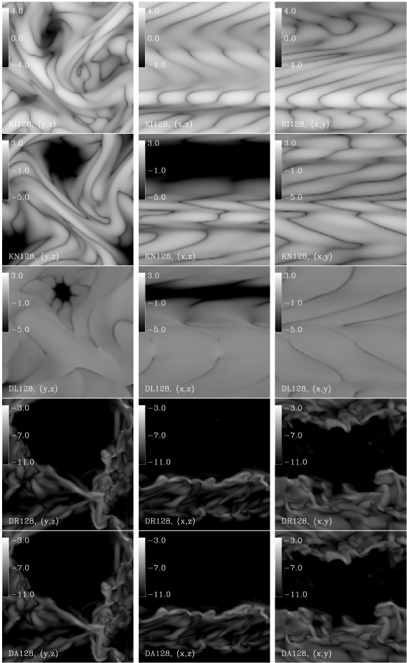
Figure 3: Logarithm of magnetic energy density at midplane, in planes $(y,z)$ (left), $(x,z)$ (center) and $(x,y)$ (right). Models from top to bottom: KI, KN, DL, DR and DA. For model names, see Table 1.

More dramatic changes come with the inclusion of the Lorentz force, but not the Reynolds stress (third row of Figure 3, models DL). Although Figure 2 shows that the magnetic field is still some way from saturation, and the magnetic energy is indistinguishable from that of the kinematic models,the spatial intermittency and amount of folding are markedly reduced.

The final two rows, models DR and DA, show how the small scale flow generated by nonlinear advection affects the magnetic field. The ordered orientation associated with the strong shear in the GP flow is essentially gone. Since there is little dynamo action, magnetic feedback is unimportant, and the magnetic fields in the two cases are virtually identical. Although there has been little amplification of the field as a whole, there are thin filaments where it is locally strong. These structures are associated with strong compression (negative divergence in the ion velocity) and with strong vorticity.

Magnetic energy spectra for the KI, KN, and DL models at a linear resolution of $N=256$ are shown in Figure 4. Although there is a slight reduction of power at the smallest scales it is not as important as the overall diminished amplitude and it is clear that power spectra without phase information give an incomplete picture of the structure of the magnetic field.

Figure 4: Power spectra of the magnetic energy for models KI, KN and DL at a linear resolution of $N=256$, and at system time $t=16$, i.e. at a point when the energy evolution of models KN and DL has separated due to saturation (see Fig. 2).

4 Discussion and Summary

Galactic magnetic fields show considerable long range order, while computations of small scale turbulent dynamos in highly conducting plasmas have shown instead that magnetic energy is concentrated at the resistive scale. This suggests that there must be some feature of the interstellar dynamo which suppresses growth of the small scale field, and that there exist mechanisms for transferring energy to scales larger than the turbulent injection scale.

In this paper we investigated the role of ion-neutral friction in eliminating the smallest scales. We solved a simple model problem in which the neutral flow was known to be a dynamo, and was coupled to the plasma through frictional drag. The plasma flow was determined by friction, inertia, and Lorentz forces. Ionization equilibrium was assumed. We used a spatially constant Ohmic resistivity, and we relied on viscous dissipation at the resolution scale.

This study is, as far as we know, the first dynamo model in which the plasma flow is calculated from the full equation of motion, rather than assuming the strong coupling approximation (Shu 1983). The strong coupling approximation breaks down at small scales, and leads to an equation for magnetic energy growth which differs somewhat from the standard equation in a plasma [compare equations (1) and (3)]. However, our models differ from the interstellar medium in several significant respects, due to the prohibitively large computational resources required for a realistic simulation. In the models, the neutral forcing occurs on timescales comparable to the ion-neutral collision time, whereas in the diffuse, weakly ionized interstellar medium the shortest timescale in neutral turbulence is probably 2-3 orders of magnitude longer. This introduces an artificially large difference between $\mathbf{v}_{i}$ and $\mathbf{v}_{n}$. By taking the magnetic diffusivity larger than the viscous diffusivity (small magnetic Prandtl number $P_{m}$), we reverse the interstellar ordering ($P_{m}\gg 1$). By assuming ionization equilibrium, an isothermal equation of state, and a uniform density of neutrals, we preclude the possibility of plasma pressure gradients. And finally, the resistive scale is only about two orders of magnitude less than the dynamical scale, instead of 5-6, as in the ISM.

Our work does not address the growth of the field at the largest scales. Whether ambipolar diffusion acting on small scale turbulence can drive a large scale field, either by quasilinear (Zweibel 1988, Proctor & Zweibel 1992) or nonlinear (Subrahmanian 1997, 1999, Brandenburg & Subrahmanian 2000) effects cannot be probed by our study due to the large range of scales that would be required, and also, perhaps, because the neutral velocity is already a dynamo.

Our main results are as follows. First, friction successfully imprints a dynamo flow on the ions, despite the importance of inertial terms [models KN; Fig. (2)]. That is, computing $\mathbf{v}_{i}$ from equation (10) leads to a flow which amplifies a weak magnetic field. Second, adding nonlinear advection ($\mathbf{v}_{i}\cdot\mathbf{\nabla}\mathbf{v}_{i}$) to equation (10) results in an ion flow which does not amplify the magnetic field, except in thin regions with large vorticity or negative divergence [models DR; Fig. (3)]. This may be a manifestation of the difficulty of driving a dynamo when $P_{m}\ll 1$, or in a highly compressible medium. It would not necessarily carry over to the diffuse ISM, in which $P_{m}$ is large and the recombination time is longer than the eddy turnover time. Third, when the Lorentz force is added, but the Reynolds stress is dropped, the dynamo saturates when the magnetic energy is about two orders of magnitude less than the plasma kinetic energy [models DL; Fig. (2)]. According to conventional wisdom, the magnetic energy saturates only close to equipartition; the difference here is due to the spatial intermittency of the magnetic field, which allows Lorentz forces to become strong just where the field is being amplified. Finally, adding the Lorentz force suppresses small scale structure (Fig. 3).

The saturation reported here for models without nonlinear advection (models DL) has some features in common with the study by Tanner & Hughes (2003), although these authors considered fully ionized systems. They studied a superposition of the GP flow (which they call the CP, or Circularly Polarized flow) and a steady flow known to be a slow dynamo, restricted the dynamics by omitting the Reynolds stress term and averaged the Lorentz force over what in our case would be the $x$ direction. They found that when the GP flow dominates, saturation occurs through suppression of exponential field line stretching by Lorentz forces, rather than by enhanced dissipation brought about by an increase in small scale structure.

Taken at face value, our computations suggest that in weakly ionized gases, the efficiency of dynamos is reduced at scales below the neutral-ion coupling length. The main point is that saturation of the field at small scales is determined by the kinetic energy in the plasma at these scales rather than in the bulk medium. The inertia of the neutrals contributes, and presumably increases the saturation level, only for motions with turnover time $\tau_{l}$ greater than the neutral-ion collision time $\tau_{ni}\equiv(\rho_{i}\gamma_{in})^{-1}$. If we take $n_{i}\sim 2\times 10^{-3}$ cm^-3, representative of both cold and warm neutral interstellar gas, then $\tau_{ni}\sim 3\times 10^{11}$s. Taking the expressions for Kolmogorov turbulence given in §2.1, and assuming the driving scale and velocity are 10 pc and 10 km s^-1, respectively, we find $\tau_{l}\sim\tau_{ni}$ at $l\sim 10^{-2}$pc. The equipartition magnetic field strength at this scale relative to the ions is only $\sim.02\mu G$, or about 1% of the Galactic value. Thus, saturation of the dynamo below the neutral-ion decoupling scale could prevent amplification of the field at very small scales.

At early times, when the magnetic field might have been several orders of magnitude or more weaker than it is today, the decoupling effect would have been less important. Furthermore, the interstellar medium was probably almost fully ionized until metallic coolants had mixed into it. Thus, the mechanisms addressed here are probably more relevant to the maintenance of galactic magnetic fields than to their ultimate origin.

References

- Boldyrev & Cattaneo (2004) Boldyrev, S. & Cattaneo, F. 2004, Phys. Rev. Lett., 92, 144501
- Brandenburg & Subramanian (2000) Brandenburg, A. & Subramanian, K. 2000, å, 361, L33
- Brummell, Cattaneo & Tobias (2001) Brummell, N. H., Cattaneo, F., Tobias, S. M. 2001, Fl. Dyn. Res., 28, 237
- Cameron & Galloway (2005) Cameron, R. & Galloway, D. 2005, MNRAS, 358, 1025
- Cattaneo, Hughes, & Kim (1996) Cattaneo, F., Hughes, D.W., & Kim, E-J. 1996, Phys. Rev. Lett., 76, 2057
- Childress & Gilbert (1995) Childress, F. & Gilbert, A.D. 1995, Stretch, Twist, Fold: The Fast Dynamo, Springer
- Courvoisier, Hughes, & Tobias (2006) Couvoisier, A., Hughes, D.W. & Tobias, S.M. 2006, PRL, 96, 034503
- Galloway & Proctor (1992) Galloway, D. J. & Proctor, M. R. E. 1992, Nature, 356, 691
- Gilbert (2002) Gilbert, A.D. 2002, Phys. Rev. D, 166, 167
- Goldreich & Sridhar (1995) Goldreich, P. & Sridhar, S. 1995, ApJ, 438, 763
- Goldreich & Sridhar (1997) Goldreich, P. & Sridhar, S. 1997, ApJ, 485, 680
- Haugen, Brandenburg, &Mee (2004) Haugen, N.E., Brandenburg, A., & Mee, A.J. 2004, MNRAS, 353, 947
- Heitsch et al. (2007) Heitsch, F., Slyz, A.D., Devriendt, J.E.G., Hartmann, L.W., Burkert, A. 2007, ApJ, 665, 445
- Heitsch & Zweibel (2003a) Heitsch, F. & Zweibel, E.G. 2003, ApJ, 583, 229
- Heitsch & Zweibel (2003b) Heitsch, F. & Zweibel, E.G. 2003, ApJ, 590, 291
- Heitsch et al. (2004) Heitsch, F., Zweibel, E.G., Slyz, A.D., Devriendt, J.E.G. 2004, ApJ, 603, 165
- Kim (1997) Kim, E-J. 1997, ApJ, 477, 183
- Klapper & Young (1995) Klapper, I.M. & Young, L.S. 1995, Comm Math Phys 173, 623
- Kulsrud & Anderson (1992) Kulsrud, R.M. & Anderson, S.W. 1992, ApJ, 396, 606
- Kulsrud & Zweibel (2008) Kulsrud, R.M. & Zweibel, E.G. 2008, astro-ph/0707.2783
- Moffatt (1978) Moffatt, H.K. 1978, in Magnetic field generation in electrically conducting fluids, Cambridge Univ. Press, Cambridge
- Ott (1998) Ott, E. 1998, Phys. Pl. 5, 1636
- Proctor & Zweibel (1992) Proctor, M.R.E. & Zweibel, E.G. 1992, GAFD, 64, 145
- Schekochihin et al. (2004) Schekochihin, A.A., Cowley, S.C., Taylor, S.F., Maron, J.L., & McWilliams, J.C. 2004, ApJ, 612, 276
- Schekochihin et al. (2007) Schekochihin, A.A., Isakov, A.B., Cowley, S.C., McWilliams, J.C., Proctor, M.R.E., & Yousef, T.A. 2007, New J Phys, 9, 300
- Shu (1983) Shu, F.H. 1983, ApJ, 273, 202
- Sridhar & Goldreich (1994) Sridhar, S. & Goldreich, P. 1994, ApJ, 432, 612
- Subramanian (1997) Subramanian, K. 1997, arXiv:astro-ph/9708216
- Subramanian (1999) Subramanian, K. 1999, PRL, 83, 2957
- Tanner & Hughes (2003) Tanner, S.E.M. & Hughes, D.W. 2003, ApJ, 586, 685
- Tang & Xu (2000) Tang, H. Z. & Xu, K. 2000, J. Comp. Phys., 165, 69
- Xu (1999) Xu, K. 1999, J. Comp. Phys., 153, 334
- Zweibel (1988) Zweibel, E.G. 1988, ApJ, 329, 384